Non-minimal Coupling Branes

Yu-Xiao Liu, Feng-Wei Chen, Heng Guo, Xiang-Nan Zhou Note: Corresponding author Affiliation: Institute of Theoretical Physics, Lanzhou University,
Lanzhou 730000, People’ s Republic of China Email: liuyx@lzu.edu.cn, chenfw10@lzu.edu.cn, guoh2009@lzu.cn, zhouxn10@lzu.edu.cn

Abstract

We study a thick and $\mathbb{Z}_{2}$ symmetric braneworld model with a non-minimally coupled bulk scalar. Several analytic solutions are found. There are two categories of the brane configuration: standard branes and deformed ones. The former is just the same with the solutions in general relativity, whereas the latter has negative effective energy densities in the location of the branes. The question of stability under metric tensor perturbation is also investigated, and there is no tachyon. We show that the gravity zero mode (namely the 4D massless graviton) is the only one state that can be localized on the branes. So Newtonian potential can be recovered in 4D space-time.

Keywords

Field Theories in Higher Dimensions, Large Extra Dimensions

1 Introduction

In the 60’s of 20th century, Brans and Dicke proposed that in gravity theory there should exist a scalar field according to Mach’s principle. From then on, both Brans-Dicke theory and general relativity are generally held to be in agreement with observations. The Brans-Dicke theory has been generalized to the so-called scalar-tensor theory of gravity (see a comprehensive book [1]). In string/M theories, there is also a scalar field (dilaton), which is non-minimally coupled to gravity. Therefore, string/M theories give the scalar-tensor theory¹¹ 1 In this paper, we ignore the difference between the scalar-tensor theory and the non-minimal theory of gravity. rather than general relativity. It has been shown that various $F(R)$ theories are also equivalent to non-minimal coupling theories (see e.g. [2]). Furthermore, non-minimally coupled theories can also originate from multi-dimensional theories, quantum field theory in curved space-time, and induced gravity theories.

In a general gravity theory with a non-minimally coupled scalar, higher derivative terms can also be included. The action is written as

S=\int_{M}\sqrt{-g}d^{n}x\left[\mathfrak{L}_{g}(f(\phi,X)R,R^{AB}\partial_{A}\phi\partial_{B}\phi,\cdots)+\mathfrak{L}_{m}(X,\phi)\right],

(1)

where $X=-g^{AB}\partial_{A}\phi\partial_{B}\phi$ . However, the general action is difficult to deal with since the corresponding equations of motion are higher derivative equations. In this paper, we would like to investigate the non-minimal coupling thick braneworld model in 5-dimensional space-time, and the action is chosen as

S=\int_{M}\sqrt{-g}d^{5}x\left[\frac{F(\phi)}{16\pi G_{5}}R+\mathfrak{L}_{m}(X,\phi)\right].

(2)

This action does not lead to more complicated equations of motion in principle. We do not cost too much to solve the problem. If $F(\phi)=e^{\gamma\phi}$ , the scalar is a dilaton. This model has a close relation with Weyl geometry, which has been extensively studied.

On the other hand, the idea that we live on a brane [3, 4, 5, 6] has received a lot of attention in recent years. Braneworld models have revealed new possibilities for addressing the hierarchy problem of particle physics as well as cosmological constant problem. Thin braneworld models, such as the Arkani-Hamed-Dimopoulos-Dvali (ADD) model [4] and the Randall-Sundrum (RS) models [5, 6], were inspired by D-brane theory. While, thick branes, which are usually generated by scalar fields, were proposed as a generalization of thin branes [7, 8, 9, 10, 11], (see a recent review [12] and references therein). In thick braneworld model, the Standard Model (SM) matter fields are confined dynamically on the brane.

It is natural to consider braneworld models with non-minimally coupled background scalar [13, 14, 15, 16, 17, 18, 19, 20, 21, 22, 23, 24, 25], since braneworld models were inspired by string theories. Several exact RS metric solutions were obtained in [15, 16, 13]. The models with a special form $F(\phi)=1-\alpha\phi^{2}$ have been studied in various papers [13, 14, 15, 16, 17, 18, 19, 20, 21, 22]. Several exact RS metric solutions were obtained in [15, 16, 13]. Some thick brane solutions were also given in [13]. The accurate perturbation equation was given in [14]. In [14], the effect Newtonian potential for RS metric branes was calculated by the technic of the bent brane [26, 27]. Moreover, a non-minimally coupled Phantom bulk field was considered in [21].

Whereas, all results were based on the special form, and no general information was given in the previous papers. We cannot finger out whether those results are dependent on the special choice. For other functions $F(\phi)$ , no exact solution is provided. Therefore, in the present article a general non-minimal coupling $F(\phi)$ is taken into account. We consider a static $\mathbb{Z}_{2}$ symmetric flat 3-brane embedded in 5D space-time and an ordinary kink scalar field is non-minimally coupled to gravity.

In the following section, we introduce the model and fundamental properties of $F(\phi)R$ gravity. In section 3, some exact solutions are given, and the behavior of the asymptotic space-time is also studied. In section 4, we investigate the problem of stability. As expected, there is no tachyon for the gravitational perturbation. We list our main results in the last section.

2 The model

In this paper, we consider a five-dimensional gravity theory with a non-minimally coupled bulk scalar field. The action takes the following form

S=\int d^{4}xdy\sqrt{-g}\left(\frac{1}{2}F(\phi)R-\frac{1}{2}(\partial\phi)^{2}-V(\phi)\right)+\int d^{4}x\sqrt{-g^{(\text{brane})}}\lambda(\phi),

(3)

where $(\partial\phi)^{2}=g^{AB}\partial_{A}\phi\partial_{B}\phi$ . For convenience we set $8\pi G_{5}=M_{5}^{-3}=1$ , $x^{5}=y$ . The kinematics of the scalar field is standard. If $F(\phi)$ is positive, it describes gravity; negative, anti-gravity. If there exists anti-gravity, there would be forces of repulsion between matter fields in this region. This leads to the result that matter distribution may be unstable. So we assume that $F(\phi)$ is a general smooth non-negative function and its zero points lie only at infinity if they exist. This is a restriction of the scalar-tensor theory. Furthermore, at the location of the brane $F=1$ is satisfied. Thin brane solutions have been studied in [13] [14]. In the following we consider thick brane scenario, so the four-dimensional part in (3) vanishes.

By setting $\Phi=F(\phi)$ , we can write the action (3) as

S=\int d^{4}xdy\sqrt{-g}\left[\frac{1}{2}\Phi R-\frac{\omega(\Phi)}{\Phi}(\partial\Phi)^{2}-\tilde{V}(\Phi)\right],

(4)

where the Brans-Dicke parameter $\omega(\Phi)=\frac{F}{2F_{\phi}^{2}}$ with $F_{\phi}\equiv\partial_{\phi}F(\phi)$ .

We have two ways to solve the field equations of the scalar-tensor gravity theory. The first one is to make a conformal transformation to recover Einstein frame:

$\displaystyle\tilde{g}_{AB}$	$\displaystyle=$	$\displaystyle e^{2\omega}g_{AB}=F^{2/3}g_{AB},$	(5)
$\displaystyle\tilde{R}$	$\displaystyle=$	$\displaystyle e^{-2\omega}(R-8\nabla^{2}\omega-12(\partial\omega)^{2}),$	(6)
$\displaystyle S$	$\displaystyle=$	$\displaystyle\int d^{4}xdy\sqrt{-\tilde{g}}\Bigg[\frac{1}{2}\tilde{R}-\frac{1}{2}\left(\frac{4F_{\phi}^{2}}{3F^{2}}+\frac{1}{F}\right)\tilde{g}^{AB}\partial_{A}\phi\partial_{B}\phi-F^{5/3}V(\phi)\Bigg].$	(7)

Defining a new scalar field

\xi=\int d\phi\sqrt{\frac{4F_{\phi}^{2}}{3F^{2}}+\frac{1}{F}},

(8)

we arrive at

S=\int d^{4}xdy\sqrt{-\tilde{g}}\left[\frac{1}{2}\tilde{R}-\frac{1}{2}\tilde{g}^{AB}\partial_{A}\xi\partial_{B}\xi-\tilde{V}(\xi)\right]

(9)

with $\tilde{V}=F^{5/3}(\phi(\xi))\;V(\phi(\xi))$ . Thus, the problem in the scalar-tensor gravity is transferred as solving the field equations in Einstein frame and the transformation (8).

The second way, which is the one we will adopt in this paper, is to solve the following modified Einstein equations straightly

F(\phi)\big(R_{AB}-\frac{1}{2}g_{AB}R\big)+(g_{AB}\nabla^{2}-\nabla_{A}\nabla_{B})F(\phi)=T^{(\phi)}_{AB},

(10)

where $T^{(\phi)}_{AB}=\partial_{A}\phi\partial_{B}\phi-g_{AB}\left(\frac{1}{2}(\partial\phi)^{2}+V\right)$ is the energy-momentum tensor of the scalar field. We can write them in a standard form:

R_{AB}-\frac{1}{2}g_{AB}R=T_{AB}^{\text{eff}}

(11)

with the effective energy-momentum tensor $T_{AB}^{\text{eff}}=\big[T^{(\phi)}_{AB}-(g_{AB}\nabla^{2}-\nabla_{A}\nabla_{B})F(\phi)\big]/F(\phi)$ .

In the following, we use another version of the modified Einstein equations (10):

\displaystyle F(\phi)R_{AB}-(\nabla_{A}\nabla_{B}+\frac{1}{3}g_{AB}\nabla^{2})F(\phi)=\bar{T}^{(\phi)}_{AB},

(12)

where

\displaystyle\bar{T}^{(\phi)}_{AB}=T^{(\phi)}_{AB}-\frac{1}{3}g_{AB}T^{(\phi)}=\partial_{A}\phi\partial_{B}\phi+\frac{2}{3}g_{AB}V(\phi).

(13)

The equation of motion for the scalar field is

\nabla^{2}\phi+\frac{1}{2}F_{\phi}(\phi)R-V_{\phi}(\phi)=0.

(14)

The metric of a thick brane model is usually assumed as follows ²² 2 $A,B$ run for all 5D indices, $\mu,\nu$ for 4D ones.

\displaystyle ds^{2}=g_{AB}dx^{A}dx^{B}=e^{2A(y)}\hat{g}_{\mu\nu}(x)dx^{\mu}dx^{\nu}+dy^{2},

(15)

where $\hat{g}_{\mu\nu}(x)$ is the induced metric on the brane. The scalar curvature is

\displaystyle R=e^{-2A(y)}\hat{R}-8A^{\prime\prime}(y)-20A^{\prime 2}(y),

(16)

where $\hat{R}$ is the Ricci scalar calculated by the induced metric $\hat{g}_{\mu\nu}$ . The four-dimensional Newton’s gravity constant $G_{4}$ is obtained by the dimensional reduction (here we recover the 5-dimensional Newton’s constant)

\frac{1}{8\pi G_{4}}=M_{p}^{2}=\frac{1}{8\pi G_{5}}\int^{+\infty}_{-\infty}dye^{2A(y)}F(\phi(y)).

(17)

In order to construct a static flat thick brane, we use the following metric

ds^{2}=e^{2A(y)}\eta_{\mu\nu}dx^{\mu}dx^{\nu}+dy^{2},

(18)

which has four-dimensional Poincaré symmetry. Then the modified Einstein equations (12) read

	$\displaystyle 3F(\phi(y))(4A^{\prime 2}+A^{\prime\prime})+7A^{\prime}F^{\prime}(\phi(y))+F^{\prime\prime}(\phi(y))$	$\displaystyle=$	$\displaystyle-2V,$		(19)
	$\displaystyle 3F(\phi(y))A^{\prime\prime}-A^{\prime}F^{\prime}(\phi(y))+F^{\prime\prime}(\phi(y))+\phi^{\prime 2}$	$\displaystyle=$	$\displaystyle 0.$		(20)

Here the prime denotes the derivative with respect to $y$ . And the equation of motion for the scalar field (14) reads

\phi^{\prime\prime}+4A^{\prime}\phi^{\prime}-2F_{\phi}(\phi)(2A^{\prime\prime}+5A^{\prime 2})-V_{\phi}(\phi)=0.

(21)

Among the above three equations (19)-(21), only two are independent.

In general relativity, BPS solutions can simplify Einstein equations. We can obtain solutions from the following way. First, we set

\displaystyle\phi^{\prime}=W(\phi),\quad A^{\prime}=P(\phi).

(22)

Then eq. (20) becomes

\displaystyle 3FP_{\phi}-PF_{\phi}+(F_{\phi\phi}+1)W+F_{\phi}W_{\phi}=0,

(23)

and the scalar potential is given by

V=\frac{1}{2}W^{2}-6P^{2}F-4PWF_{\phi}.

(24)

3 The solutions

In conventional thick brane theory, there is a scalar field with a proper symmetry-breaking potential as an order parameter. So we often choose the scalar field as a kink solution. The kink interpolates between two anti-de Sitter vacua, at which the scalar potential reaches its (local) minimal values. However, there is some subtle difference for the non-minimally coupled theory, since the term $F(\phi)R$ contributes an effective potential for the scalar field. We can choose proper functions $F(\phi)$ and $V(\phi)$ to construct various branes.

3.1 The asymptotic property of the warp factor

In this paper we mainly study symmetric thick branes generated by a single kink scalar. So we choose that $\phi(y)$ is an odd function and $A(0)=A^{\prime}(0)=0$ . It imposes the constraint that $F(\phi)$ and $V(\phi)$ are even functions of $\phi$ .

From eq. (20), it is easy to obtain

A^{\prime\prime}(0)=-\frac{1}{3}\big[F^{\prime\prime}(\phi(0))+\phi^{\prime}(0)^{2}\big]=-\frac{1}{3}\big[F_{\phi\phi}(\phi(0))+1\big]\phi^{\prime}(0)^{2}.

(25)

Here we only consider the single kink scenario, hence $\phi^{\prime}(0)^{2}>0$ . With the help of eq. (19), we have the effective energy density:

\displaystyle\rho_{\text{eff}}=-g^{00}T_{00}^{\text{eff}}=\frac{1}{2F}\left(\phi^{\prime 2}+F^{\prime\prime}-3A^{\prime\prime}F+3A^{\prime}F^{\prime}-12A^{\prime 2}F\right).

(26)

If $F_{\phi\phi}(\phi(0))>-1$ , then $A^{\prime\prime}(0)<0$ and we will get a usual single brane just like in the standard thick brane case. If $F_{\phi\phi}(\phi(0))<-1$ , then $A^{\prime\prime}(0)>0$ and the brane will be split into two positive tension sub-branes located around $y=0$ and a negative tension sub-brane located at $y=0$ , which cannot be constructed in conventional general relativity.

As is well known, in Einstein’s gravity, a kink solution will result in an asymptotic AdS space-time. Now we analyze the asymptotic space-time in the non-minimally coupled theory considered in the paper.

For given $F(\phi)$ and $\phi(y)$ , $A^{\prime}(y)$ can be calculated by

	$\displaystyle A^{\prime}(y)$	$\displaystyle=$	$\displaystyle-\frac{1}{3}F^{\frac{1}{3}}(\phi(y))\int_{0}^{y}F^{-\frac{4}{3}}(\phi(\bar{y}))\Big[F^{\prime\prime}(\phi(\bar{y}))+\phi^{\prime 2}\Big]d\bar{y}$		(27)
		$\displaystyle=$	$\displaystyle-\frac{F^{\prime}(\phi(y))}{3F(\phi(y))}-\frac{1}{3}F^{\frac{1}{3}}(\phi(y))\int_{0}^{y}\Big[\frac{4F^{\prime 2}(\phi(\bar{y}))}{3F^{\frac{7}{3}}(\phi(\bar{y}))}+\frac{\phi^{\prime 2}(\bar{y})}{F^{\frac{4}{3}}(\phi(\bar{y}))}\Big]d\bar{y}.$		(28)

Here we assume that $F(\phi)$ is an even smooth function of $\phi$ . If $F(\phi(y))$ tends to infinity when $y\rightarrow\infty$ , the warp factor $e^{2A(y)}<F^{-2/3}(\phi(y))$ and vanishes. If $F(\phi(\infty))$ is a positive constant (notice that $F^{\prime}(\phi(0))=0$ ), we would have

\displaystyle A^{\prime}(+\infty)=-\frac{1}{3}F^{\frac{1}{3}}(\phi(+\infty))\int_{0}^{+\infty}\Big[\frac{4F^{\prime 2}(\phi(\bar{y}))}{3F^{\frac{7}{3}}(\phi(\bar{y}))}+\frac{\phi^{\prime 2}(\bar{y})}{F^{\frac{4}{3}}(\phi(\bar{y}))}\Big]d\bar{y}.

(29)

From the above equation we know that $A^{\prime}(+\infty)$ is a negative constant, so the scalar curvature tends to a negative constant at infinity, and the space-time is asymptotic AdS. This is a general conclusion. This conclusion can be confirmed by the way of the conformal transformation.

In the following, we study the possible category of the asymptotic space-times when $F(\phi(\infty))=0$ . One may expect that there exists asymptotic Minkowski space-time for proper $F(\phi)$ and $V(\phi)$ , since the contribution of gravity could vanish at infinity. While, for a kink solution, the warp factor $A(y)$ cannot be a finite constant at infinity. Hence, the space-time is asymptotic Minkowski in the sense that the scalar curvature is zero at infinity.

The second term of eq. (29) makes $A(y)$ descend faster, so in the following we mainly concentrate on the first term. We assume $F(\phi(y))$ can be expanded at infinity:

F\sim a|y|^{-b},\quad|y|\rightarrow+\infty,

(30)

where $a>0$ , $b>0$ , and ’ $\sim$ ’ denotes that we omit the higher order terms of $(y^{-b})$ .

For the case $b>3$ , though the integral $\int_{0}^{+\infty}dyF^{-\frac{4}{3}}(y)F^{\prime\prime}(y)$ in (27) is divergent, we have the asymptotic form of $A^{\prime}(y)$ for large $y$

A^{\prime}(y)\sim-\frac{1}{3}F^{\frac{1}{3}}(y)\int_{0}^{y}d\bar{y}F^{-\frac{4}{3}}(\bar{y})F^{\prime\prime}(\bar{y})\sim-\frac{b(b+1)}{b-3}y^{-1}<0,~~y\rightarrow+\infty.

(31)

This term leads that $A(y)\sim-\frac{b(b+1)}{b-3}\ln|y|$ is negative infinity.

When $b=3$ , we can get by simple calculation

	$\displaystyle A^{\prime}(y)$	$\displaystyle\sim$	$\displaystyle-\frac{\ln y}{3y},\quad y\rightarrow+\infty,$		(32)
	$\displaystyle A(y)$	$\displaystyle\sim$	$\displaystyle-(\ln\|y\|)^{2}/3,\quad\|y\|\rightarrow+\infty.$		(33)

For $b<3$ , the first term of eq. (29) is convergence, but the property of $A^{\prime}(y)$ at infinity is also mainly determined by the asymptotic expansion of $F(y)$ . From eq. (28), we have

A^{\prime}(y)\sim\frac{b}{3y}-Cy^{-\frac{b}{3}},\quad y\rightarrow+\infty,

(34)

where $C$ is a positive integration constant. Since $y^{-1}$ descends faster than $y^{-\frac{b}{3}}$ ,

A(y)\sim-C(1-\frac{b}{3})|y|^{1-\frac{b}{3}},~~y\rightarrow+\infty.

(35)

Extending $b\rightarrow 0$ , we get

A(y)\sim-C|y|,~~|y|\rightarrow+\infty.

(36)

This agrees with the conclusion obtained from the situation in which $F(\phi(y))$ is a positive constant at infinity.

From the above discussion we know that the asymptotic property of $A^{\prime}(|y|\rightarrow\infty)$ is mainly determined by $F(\phi(y))$ and $\phi(y)$ at infinity. In all above cases, $A^{\prime}(|y|\rightarrow\infty)$ approaches to zero, however $A(|y|\rightarrow\infty)$ tends to negative infinity.

We can prove that for $F(\phi(y))\sim e^{-a|y|^{b}}$ or $F(\phi(y))\sim a|y|^{-b}(\ln|y|)^{c}$ when $|y|$ tends to infinity, the warp factor $e^{2A(y)}$ vanishes. We conjecture that in our brane model the warp factor $e^{2A(y)}$ should vanish (It could be a positive constant as an extreme result). Nevertheless, we cannot find a formula to prove this for general functions.

3.2 The standard solutions

Exact solution 1:

A kink solution was given by Bogdanos, Dimitriadis and Tamvakis in [13]. In this solution, $F(\phi)=1-\alpha\phi^{2}$ with $\alpha$ a dimensionless constant, and the scalar and the warp factor are given by

	$\displaystyle\phi$	$\displaystyle=$	$\displaystyle\phi_{0}\tanh\kappa y=\sqrt{\frac{3(1-6\alpha)}{\alpha(1-2\alpha)}}\tanh(\kappa y),$		(37)
	$\displaystyle A$	$\displaystyle=$	$\displaystyle(\alpha^{-1}-6)\ln\cosh(\kappa y),$		(38)

where $\phi_{0}=\sqrt{\frac{3(1-6\alpha)}{\alpha(1-2\alpha)}}$ . This solution is only valid for the range $0<\alpha<\frac{1}{6}$ . The potential for the scalar field is

\displaystyle V(\phi)=\frac{\kappa^{2}}{6\alpha}\Big[\frac{9-54\alpha}{1-2\alpha}+6\left(\alpha(7+24\alpha)-2\right)\phi^{2}+\frac{\alpha(1-2\alpha)(3-16\alpha)(4-21\alpha)}{1-6\alpha}\phi^{4}\Big],

(39)

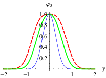
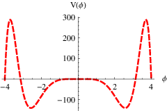
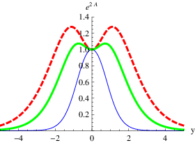
which is a $\phi^{4}$ potential. In the range $0<\alpha<\frac{1}{6}$ , the coefficient of $\phi^{4}$ term is positive. It is easy to verify that $V(\phi(y))$ doesn’t reach vacuum values when $y$ tends to infinity. From Fig. 1, we know that $\alpha$ can be taken as the parameter that describes the degree of symmetry breaking: when $\alpha$ becomes smaller, the symmetry is broken more obviously. Whatever, the parameter $\alpha$ cannot reach $\alpha=0$ . In the general relativity,

	$\displaystyle\phi(y)$	$\displaystyle=$	$\displaystyle\phi_{0}\tanh(\kappa y),\quad A(y)=-\frac{\phi_{0}^{2}}{9}\left(2\ln\cosh\kappa y+\frac{1}{4}\tanh^{2}(\kappa y)\right),$		(40)
	$\displaystyle V(\phi)$	$\displaystyle=$	$\displaystyle\frac{1}{8}\left(\frac{\partial Q}{\partial\phi}\right)^{2}-\frac{1}{3}Q^{2},\quad Q=2\kappa\phi_{0}^{2}\left(\frac{\phi}{\phi_{0}}-\frac{1}{3}\frac{\phi^{3}}{\phi_{0}^{3}}\right).$		(41)

Refer to caption — Figure 1: The shapes of the potential $V(\phi)$ , the scalar $\phi$ and the warp factor $e^{2A}$ for the exact solution 1. The dashing red, thick green and thin blue lines correspond to $\alpha=0.05,0.10$ and 0.15, respectively. The parameter $\kappa$ is set as $\kappa=1$ .

It is easy to verify that $F(\phi(y))>0$ is satisfied only if $\frac{1}{8}\leq\alpha<\frac{1}{6}$ . Another kink solution $\phi=\frac{1}{\sqrt{\alpha}}\tanh(\kappa y)$ was reported in [12]. Numerical information about general $\alpha$ was provided in [22]. Non-kink solutions can also lead to the same warp factor [13].

Exact solution 2: Here, we give another interesting solution:

$\displaystyle F(\phi)$	$\displaystyle=$	$\displaystyle\frac{\phi_{0}^{2}}{3}+(1-\frac{\phi_{0}^{2}}{3})\cosh(\frac{\sqrt{3}\phi}{\phi_{0}}),$	(42)
$\displaystyle\phi$	$\displaystyle=$	$\displaystyle\phi_{0}\arctan(\sinh\kappa y),$	(43)
$\displaystyle A(y)$	$\displaystyle=$	$\displaystyle-\ln\cosh(\kappa y),$	(44)
$\displaystyle V(\phi)$	$\displaystyle=$	$\displaystyle\frac{1}{2}\phi_{0}^{2}\kappa^{2}\cos^{2}\frac{\phi}{\phi_{0}}+\frac{2\kappa^{2}}{\sqrt{3}}\left(3-\phi_{0}^{2}\right)\sin\frac{2\phi}{\phi_{0}}\sinh\frac{\sqrt{3}\phi}{\phi_{0}}$	(45)
		$\displaystyle-\kappa^{2}\left(2\phi_{0}^{2}+(6-2\phi_{0}^{2})\cosh\frac{\sqrt{3}\phi}{\phi_{0}}\right)\sin^{2}\frac{\phi}{\phi_{0}}.$	(45)

In order to guarantee $F>0$ , following condition is needed

0<\phi_{0}^{2}<\frac{3\cosh(\sqrt{3}\pi/2)}{3\cosh(\sqrt{3}\pi/2)-1}.

(46)

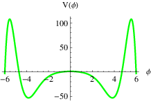
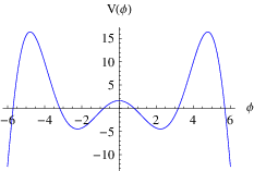
For $\phi_{0}^{2}=3$ , $F\equiv 1$ and $V(\phi)$ is the famous sine-Gordon potential, which is the case of Einstein’s gravity; $\phi_{0}^{2}<3$ , $V(\phi)$ oscillatory divergent; $\phi_{0}^{2}>3$ , $V(\phi)$ negative unlimited. From Fig. 2, we know that and $\beta=1-\frac{\phi_{0}^{2}}{3}$ can be chosen as the non-minimal coupling parameter for this solution .

From Fig. 2, we know that the potential $V(\phi)$ cannot reach its minimal values when $y$ tends to infinity. For a general solution, we have

V_{\phi}(\phi_{0})=-10P^{2}(\phi_{0})F_{\phi}(\phi_{0})

(47)

for $F(\phi_{0})\neq 0$ . Here we use $W(\phi_{0})=0$ and $\phi_{0}=\phi(+\infty)$ . Obviously in Einstein’s gravity, $V_{\phi}(\phi_{0})=0$ , so the scalar reaches vacuum value at infinity for Minkovski brane. But in non-minimally coupled theories it is not true. For the exact solution 1, $V_{\phi}(\phi_{0})>0$ since $\alpha>0$ . For the exact solution 2, $V_{\phi}(\phi_{0})<0$ if $\phi_{0}^{2}<3$ ; $V_{\phi}(\phi_{0})>0$ if $\phi_{0}^{2}>3$ .

3.3 The deformed solutions

In this subsection we give two analytic examples for the case of deformed solutions.

From eq. (28), we know if $(F(\phi))^{1/3}$ is polynomial, the result can be simplified.

Example 1:

$\displaystyle F(\phi)$	$\displaystyle=$	$\displaystyle\left(1-\frac{\phi^{2}}{\phi^{2}_{0}}\right)^{3},$	(48)
$\displaystyle\phi$	$\displaystyle=$	$\displaystyle\phi_{0}\tanh(\kappa y),$	(49)
$\displaystyle A(y)$	$\displaystyle=$	$\displaystyle-\frac{1}{24}\phi_{0}^{2}\cosh^{2}(\kappa y)-14\ln\cosh(\kappa y)+8\kappa y\tanh(\kappa y)-\frac{1}{8}\phi_{0}^{2}\kappa y\tanh(\kappa y).$	(50)

In this solution, the warp factor descends faster than the one of AdS space-time at infinity, and the scalar curvature is divergent.

Example 2: In this example, we choose $F(\phi)$ as a periodic function, and the solution is given by

$\displaystyle F$	$\displaystyle=$	$\displaystyle\cos^{2}(\frac{\phi}{\phi_{0}}),$	(51)
$\displaystyle\phi$	$\displaystyle=$	$\displaystyle\phi_{0}\arctan(\kappa y),$	(52)
$\displaystyle A(y)$	$\displaystyle=$	$\displaystyle\ln(1+\kappa^{2}y^{2})-\frac{(4+\phi_{0}^{2})\Big[\text{G}^{23}_{33}\Big(\left.{}^{1,1,\frac{7}{6}}_{\frac{2}{3},1,0}\right\|1+\kappa^{2}y^{2}\Big)-\text{G}^{23}_{33}\Big(\left.{}^{1,1,\frac{7}{6}}_{\frac{2}{3},1,0}\right\|1\Big)\Big]}{12\Gamma(\frac{2}{3})\Gamma(\frac{5}{6})},$	(53)

where $G^{23}_{33}$ is the Meijer G function, which is expanded at infinity as

\text{G}^{23}_{33}\Big(\left.{}^{1,1,\frac{7}{6}}_{\frac{2}{3},1,0}\right|1+\kappa^{2}y^{2}\Big)=\frac{1}{\Gamma(\frac{5}{6})}\left[\frac{\pi^{5/2}(\kappa y)^{\frac{1}{3}}}{\Gamma(\frac{2}{3})\Gamma(\frac{7}{6})}-\frac{1}{2}\Gamma(-\frac{1}{6})\ln(\kappa y)\right]+\mathcal{O}(1),y\rightarrow+\infty.

(54)

So the warp factor is converge. This is consistent with our analysis. The warp factors of examples 1 and 2 are depicted in Fig. 3.

Some deformed solutions were given by numerical calculation in [13, 22]. In this subsection, we obtain analytic solutions. From Fig. 3, we know that branes are standard when $\phi_{0}$ is small enough; and they become deformed as $\phi_{0}$ increases. It is a natural result because of above discussion.

4 Localization of gravitation

In the braneworld theory, it is an important problem whether the metric perturbation can be localized on the brane [7, 14, 13, 27, 26, 28, 29, 30, 31]. In five-dimensional Minkowski space-time, the gravitational potential is proportional to $r^{-2}$ according to Gauss law. However, in general, braneworld models exhibit a four-dimensional massless graviton which is localized on the brane. So Newtonian potential can be reproduced.

In this section, we check the stability of the model under the metric tensor perturbation. It is convenient to consider axial gauge condition: $h_{5A}=0$ ³³ 3 In other words, vector perturbation vanishes. However scalar perturbation is kept.. Under this gauge condition the perturbed metric is

ds^{2}=e^{2A}(\eta_{\mu\nu}+h_{\mu\nu})dx^{\mu}dx^{\nu}+dy^{2}.

(55)

We can expand modified Einstein equations to first order:

	$\displaystyle FR^{(1)}_{AB}-e^{2A}\left(\frac{2}{3}h_{AB}V+\frac{1}{2}h_{AB}^{\prime}F^{\prime}+h_{AB}A^{\prime}F^{\prime}+\frac{1}{3}h_{AB}\nabla^{2}F(\phi)\right)-\frac{1}{3}g_{AB}\left(2hA^{\prime}F^{\prime}+h^{\prime}F^{\prime}\right)$
	$\displaystyle=-F_{\phi}R_{AB}\tilde{\phi}+(\nabla_{A}\nabla_{B}+\frac{1}{3}g_{AB}\nabla^{2})(F_{\phi}\tilde{\phi})+\partial_{A}\phi\partial_{B}\tilde{\phi}+\partial_{A}\tilde{\phi}\partial_{B}\phi+\frac{2}{3}g_{AB}V_{\phi}\tilde{\phi}.$		(56)

Here $R^{(1)}_{AB}$ is the linearized Ricci tensor, $h=\eta^{\mu\nu}h_{\mu\nu}$ , and $\tilde{\phi}=\delta\phi$ .⁴⁴ 4 In this section indices $\mu,\nu$ are raised by the flat metric $\eta^{\mu\nu}$ .

$R_{AB}^{(1)}$ was calculated in [7]:

$\displaystyle R_{\mu\nu}^{(1)}$	$\displaystyle=$	$\displaystyle-e^{2A}\left[\frac{1}{2}h_{\mu\nu}^{\prime\prime}+2A^{\prime}h_{\mu\nu}^{\prime}+(A^{\prime\prime}+4A^{\prime 2})h_{\mu\nu}\right]-\frac{1}{2}\Box^{(4)}h_{\mu\nu}$	(57)
		$\displaystyle-\frac{1}{2}\eta_{\mu\nu}e^{2A}A^{\prime}h^{\prime}-\frac{1}{2}(\partial_{\mu}\partial_{\nu}h-\partial_{\mu}\partial_{\rho}h_{\nu}^{\rho}-\partial_{\nu}\partial_{\rho}h_{\mu}^{\rho}),$	(57)
$\displaystyle R^{(1)}_{55}$	$\displaystyle=$	$\displaystyle-\frac{1}{2}(h^{\prime\prime}+2A^{\prime}h^{\prime}),\quad R^{(1)}_{5\mu}=\frac{1}{2}(\partial_{\nu}h_{\mu}^{\nu}-\partial_{\mu}h)^{\prime},$	(58)

with $\Box^{(4)}=\eta^{\mu\nu}\partial_{\mu}\partial_{\nu}$ .

The fluctuation of the scalar field satisfies

\nabla^{2}\tilde{\phi}+\frac{1}{2}\phi^{\prime}h^{\prime}+\left(\frac{1}{2}F_{\phi\phi}R-V_{\phi\phi}\right)\tilde{\phi}+\frac{1}{2}F_{\phi}R^{(1)}=0.

(59)

With the help of equations of motion (19)-(20), we arrive at

$\displaystyle(\mu,\nu):$		$\displaystyle F\Big[(-\frac{1}{2}h_{\mu\nu}^{\prime\prime}-2A^{\prime}h_{\mu\nu}^{\prime}-\frac{1}{2}\frac{F^{\prime}}{F}h_{\mu\nu}^{\prime})-\frac{1}{2}e^{-2A}\Box^{(4)}h_{\mu\nu}$	(60)
		$\displaystyle-\frac{1}{2}\eta_{\mu\nu}A^{\prime}h^{\prime}-\frac{1}{3}\eta_{\mu\nu}(2hA^{\prime}+h^{\prime})\frac{F^{\prime}}{F}-\frac{1}{2}e^{-2A}(\partial_{\mu}\partial_{\nu}h-2\partial_{(\nu}h_{\mu)})\Big]$
	$\displaystyle=$	$\displaystyle\eta_{\mu\nu}\left[F_{\phi}(A^{\prime\prime}+4A^{\prime 2})\tilde{\phi}+\frac{2}{3}V_{\phi}\tilde{\phi}+\frac{1}{3}\nabla^{2}(F_{\phi}\tilde{\phi})+A^{\prime}(F_{\phi}\tilde{\phi})^{\prime}\right]+e^{-2A}F_{\phi}\partial_{\mu}\partial_{\nu}\tilde{\phi},$
$\displaystyle(5,5):$		$\displaystyle-\frac{F}{2}(h^{\prime\prime}+2A^{\prime}h^{\prime})-\frac{F^{\prime}}{3}\left(2hA^{\prime}+h^{\prime}\right)$	(61)
	$\displaystyle=$	$\displaystyle 4F_{\phi}(A^{\prime\prime}+A^{\prime 2})\tilde{\phi}+\frac{2}{3}V_{\phi}\tilde{\phi}+(F_{\phi}\tilde{\phi})^{\prime\prime}+\frac{1}{3}\nabla^{2}(F_{\phi}\tilde{\phi})+2\phi^{\prime}\tilde{\phi}^{\prime},$	(61)
$\displaystyle(5,\mu):$		$\displaystyle\frac{F}{2}\left(h_{\mu}-\partial_{\mu}h\right)^{\prime}=\phi^{\prime}\partial_{\mu}\tilde{\phi}+(F_{\phi}\partial_{\mu}\tilde{\phi})^{\prime}-A^{\prime}F_{\phi}\partial_{\mu}\tilde{\phi},$	(62)

where $h_{\mu}:=\partial^{\nu}h_{\mu\nu}$ .

4.1 Transverse Traceless component

First, let us consider the Transverse Traceless ( TT ) component $\bar{h}_{\mu\nu}$ , which is defined by

	$\displaystyle\bar{h}_{\mu\nu}:$	$\displaystyle=$	$\displaystyle\Pi_{\mu\nu\rho\sigma}h^{\rho\sigma}=(\pi_{\mu\rho}\pi_{\nu\sigma}-\frac{1}{3}\pi_{\mu\nu}\pi_{\rho\sigma})h^{\rho\sigma},$		(63)
	$\displaystyle h_{\mu\nu}:$	$\displaystyle=$	$\displaystyle\bar{h}_{\mu\nu}+h^{NT}_{\mu\nu},$		(64)

with $\pi_{\mu\nu}=\eta_{\mu\nu}-\partial_{\mu}\partial_{\nu}/\Box^{(4)}$ . $\bar{h}_{\mu\nu}$ satisfies

\partial^{\mu}\bar{h}_{\mu\nu}=\eta^{\mu\nu}\bar{h}_{\mu\nu}=0.

(65)

The TT component describes the ordinary gravitational wave and we can prove that TT component is invariant under gauge transformation. Here we introduce projection operator $\Pi_{\mu\nu\rho\sigma}$ , which has following properties:

	$\displaystyle\Pi_{\mu\nu\rho\sigma}\eta^{\rho\sigma}f_{1}(x,y)=0,$		(66)
	$\displaystyle\Pi_{\mu\nu}^{~~~\rho\sigma}\partial_{(\rho}w_{\sigma)}(x,y)=0.$		(67)

Here $f_{1}(x,y),w_{\mu}(x,y)$ are arbitrary four-dimensional scalar field and vector field, respectively.

From eqs. (66)-(86), we can know that the TT component $\bar{h}_{\mu\nu}$ is decoupled with the Non-Transverse Traceless one $h_{\mu\nu}^{NT}$ , and the fluctuation of the background scalar field $\tilde{\phi}$ just refers to the NT component $h_{\mu\nu}^{NT}$ . Using the projection operator, We get fluctuation equation for the TT component [13]:

\displaystyle\left(-\partial_{y}^{2}-(4A(y)+\ln F(\phi(y)))^{\prime}\partial_{y}-e^{-2A}\Box^{(4)}\right)\bar{h}_{\mu\nu}=0.

(68)

If $F=0$ for some $y$ , the stability would have trouble. This coincides with the analysis in section 2.

We can eliminate the factor $e^{2A}$ in conformally flat coordinates:

ds^{2}=e^{2A(z)}[(\eta_{\mu\nu}+h_{\mu\nu})dx^{\mu}dx^{\nu}+dz^{2}],~~~~dz=e^{-A}dy.

(69)

Now eq. (68) yields

\left(-\partial_{z}^{2}-3\dot{A}_{E}(z)\partial_{z}-\Box^{(4)}\right)\bar{h}_{\mu\nu}=0.

(70)

Here $A_{E}(z)=3A(z)+\ln F(z)$ and the dot denotes the derivative with respect to $z$ .

We set $\bar{h}_{\mu\nu}(x,z)=e^{-3A_{E}/2}e^{ipx}e_{\mu\nu}(p)\varphi(z)$ with $e_{\mu\nu}$ satisfying $p^{\mu}e_{\mu\nu}=e^{\mu}_{~~\mu}=0$ . Then eq. (70) takes Schrödinger form:

\left(-\partial^{2}_{z}+V_{g}(z)\right)\varphi=m^{2}\varphi,

(71)

where $m$ is the four-dimensional mass satisfying $m^{2}=-p^{2}$ and the potential for the gravitons is

V_{g}(z)=\frac{3}{2}\ddot{A}_{E}(z)+\frac{9}{4}\dot{A}_{E}^{2}(z).

(72)

The effective potential for the gravitons is a volcano potential. Eq. (71) can be written as supersymmetric form

$\displaystyle L^{\dagger}L\varphi(z)$	$\displaystyle=$	$\displaystyle m^{2}\varphi(z),$	(73)
$\displaystyle L$	$\displaystyle=$	$\displaystyle\partial_{z}-\frac{3}{2}\dot{A}_{E}(z),$	(74)
$\displaystyle L^{\dagger}$	$\displaystyle=$	$\displaystyle-\partial_{z}-\frac{3}{2}\dot{A}_{E}(z).$	(75)

As the operator $L^{\dagger}L$ is hermitian and positive definite, the solution is stable under the TT perturbation, or $m^{2}\geq 0$ . The massless mode satisfies $L\varphi_{0}=0$ , and it can be normalized:

$\displaystyle\varphi_{0}$	$\displaystyle=$	$\displaystyle Ne^{3A_{E}/2}=Ne^{3A(z)/2}F(z)^{1/2},$	(76)
$\displaystyle\int^{+\infty}_{-\infty}dz\varphi_{0}^{2}(z)$	$\displaystyle=$	$\displaystyle N^{2}\int^{+\infty}_{-\infty}dze^{3A(z)}F(z)=N^{2}\frac{G_{5}}{G_{4}}=1,$	(77)
$\displaystyle N$	$\displaystyle=$	$\displaystyle\sqrt{\frac{G_{4}}{G_{5}}}.$	(78)

Here we use the definition of the 4-dimensional Newton’s gravity constant.

From eq. (28), we have

A_{E}^{\prime}(y)=-\frac{1}{9}F^{\frac{1}{3}}(\phi(y))\int_{0}^{y}\Big[\frac{4F^{\prime 2}(\phi(\bar{y}))}{3F^{\frac{7}{3}}(\phi(\bar{y}))}+\frac{\phi^{\prime 2}(\bar{y})}{F^{\frac{4}{3}}(\phi(\bar{y}))}\Big]d\bar{y}.

(79)

Unlike the warp factor, the massless graviton has its maximum value on the brane. It is clear that the zero mode is localized on the brane, which reproduces the standard Newtonian gravity on the brane.

We can give analytic expressions of the potential $V_{g}$ for the exact solution 1 with $\alpha=\frac{1}{7}$ and the exact solution 2. The metrics for both cases share the same form:

\displaystyle ds^{2}

\displaystyle=

\displaystyle\frac{1}{1+(\kappa z)^{2}}(\eta_{\mu\nu}dx^{\mu}dx^{\nu}+dz^{2}).

(80)

For the exact solution 1 with $\alpha=\frac{1}{7}$ , the potential reads

V_{g}(z)=\frac{15\kappa^{2}\left(-14+37\kappa^{2}z^{2}+28\kappa^{4}z^{4}+4\kappa^{6}z^{6}\right)}{4\left(5+7\kappa^{2}z^{2}+2\kappa^{4}z^{4}\right)^{2}}.

(81)

And the normalized zero mode is

\displaystyle\varphi_{0}(z)=\sqrt{\frac{\kappa}{8}}\frac{\sqrt{5+2\kappa^{2}z^{2}}}{\left(1+\kappa^{2}z^{2}\right)^{5/4}}.

(82)

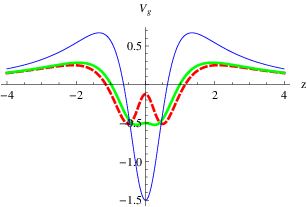
We plots the potential $V_{g}$ and the zero mode $\varphi_{0}$ for $\alpha=1/7$ in Fig. 4. For other values of $\alpha$ in the range of $\frac{1}{8}\leq\alpha<\frac{1}{6}$ , the shape of the potential for the gravitons does not change sharply.

It is interesting to note that $F(R)$ gravity has the same solution if $F(R)=R+\gamma R^{2}$ [32], and both solutions have many similar properties.

With respect to the exact solution 2, the function $F(\phi(z))$ and the potential $V_{g}(z)$ are

$\displaystyle F(\phi(z))$	$\displaystyle=$	$\displaystyle\frac{\phi_{0}^{2}}{3}+(1-\frac{\phi_{0}^{2}}{3})\cosh(\sqrt{3}\arctan(\kappa z)),$
$\displaystyle V_{g}(z)$	$\displaystyle=$	$\displaystyle\frac{\kappa^{2}}{8(1+\kappa^{2}z^{2})^{2}(\phi_{0}^{2}+3\sqrt{1-f^{2}})^{2}}\Big[45(\phi_{0}^{4}-2\phi_{0}^{2}+3)\kappa^{2}z^{2}-9(\phi_{0}^{4}+2\phi_{0}^{2}-3)$	(83)
		$\displaystyle+9\beta(5\kappa^{2}z^{2}-1)(4\phi_{0}^{2}\sqrt{1-f^{2}}+3\beta+6\beta f^{2})-{60\sqrt{3}\beta\kappa^{3}zf(\phi_{0}^{2}+3\sqrt{1-f^{2}})}\Big],~~~~~~~~$	(83)

where

\displaystyle f=\sinh(\sqrt{3}\arctan(\kappa z)),\quad\beta=1-\frac{\phi_{0}^{2}}{3}.

We find that when $\phi_{0}^{2}<\frac{23-\sqrt{337}}{4}$ , the potential $V_{g}$ is a double-well volcano potential; when $\phi_{0}^{2}>\frac{23-\sqrt{337}}{4}$ , we get a single-well volcano potential. This point is interpreted in Fig. 5.

In this solution, the property of the potential for the gravitons mainly depends on $F(\phi)$ , or more precisely, on $\phi_{0}$ , since in this solution the warp factor is fixed.

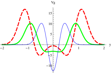
For the deformed solutions, since the non-minimal coupling function $F(\phi)$ and the warp factor $e^{2A}$ have similar properties in the examples 1 and 2, we only plot the potential $V_{g}$ for the example 1 in Fig. 6.

4.2 Non-Transverse Traceless component

Second, we consider the stability for the Non-Transverse-Traceless (NT) part.

The NT part $h^{NT}_{\mu\nu}$ is decoupled with the TT component, and is only dependent on $h_{\mu}$ and $h$ :

	$\displaystyle h_{\mu\nu}^{NT}$	$\displaystyle=$	$\displaystyle 2\partial_{(\mu}\left(\frac{1}{\Box^{(4)}}h_{\nu)}\right)+\frac{1}{3}\eta_{\mu\nu}(h-\partial_{\rho}h^{\rho})+\partial_{\mu}\partial_{\nu}\left[\frac{1}{3\Box^{(4)}}(\frac{2}{\Box^{(4)}}\partial_{\rho}h^{\rho}+h)\right],~~~~$		(84)
	$\displaystyle\eta^{\mu\rho}\partial_{\rho}h^{NT}_{\mu\nu}$	$\displaystyle=$	$\displaystyle h_{\nu},\quad\eta^{\mu\nu}h_{\mu\nu}^{NT}=h.$		(85)

From eq. (62), we know there exists a function $f(x,y)$ such that

h_{\mu}(x,y)=\partial_{\mu}f(x,y).

(86)

From eq. (86), we know that eq. (84) can be rewritten as the following form:

h^{NT}_{\mu\nu}(x,y)=2\partial_{\mu}\partial_{\nu}\Phi(x,y)+2\eta_{\mu\nu}\Psi(x,y).

(87)

Now we consider the following gauge transformation:

\displaystyle x^{\mu}\rightarrow x^{\mu}-\xi^{\mu}(x,y),\quad y\rightarrow y-\xi^{5}(x,y).

(88)

The corresponding gauge transformation for the perturbation $h_{AB}$ is: ⁵⁵ 5 In this subsection $h_{\mu\nu}^{NT}$ is written as $h_{\mu\nu}$ for short since the TT component is gauge invariant.

	$\displaystyle ds^{2}=e^{2A}(\eta_{\mu\nu}+h_{\mu\nu})dx^{\mu}dx^{\nu}+2h_{5\nu}dydx^{\nu}+(1+h_{55})dy^{2},$		(89)
	$\displaystyle h_{\mu\nu}\rightarrow h_{\mu\nu}+2\partial_{(\mu}\xi_{\nu)}+2\eta_{\mu\nu}\xi^{5},$		(90)
	$\displaystyle h_{5\nu}\rightarrow h_{5\nu}+\partial_{\nu}\xi^{5}+e^{2A}\xi_{\nu}^{\prime},$		(91)
	$\displaystyle h_{55}\rightarrow h_{55}+2(\xi^{5})^{\prime}.$		(92)

We choose the proper functions $\xi^{\mu}$ and $\xi^{5}$ to eliminate the term such as $\partial_{\mu}\partial_{\nu}\Phi$ :

	$\displaystyle\xi_{\mu}$	$\displaystyle=$	$\displaystyle-\partial_{\mu}\Phi,$		(93)
	$\displaystyle\xi^{5}$	$\displaystyle=$	$\displaystyle e^{2A}\Phi^{\prime}.$		(94)

This choice can keep the gauge condition $h_{5\mu}=0$ , however $h_{55}=0$ cannot be preserved at the same time.

Then the NT perturbation can be written in the familiar form:⁶⁶ 6 Fluctuation in this form is usually called scalar perturbation.

\displaystyle ds^{2}=e^{2A}\left[(1+2\Psi+2e^{A}\dot{\Phi})\eta_{\mu\nu}dx^{\mu}dx^{\nu}+(1+2\ddot{\Phi}+2\dot{A}\dot{\Phi})dz^{2}\right].

(95)

To simplify our discussion, we make a conformal transformation (5) (8) to recover Einstein frame:

$\displaystyle\tilde{\xi}$	$\displaystyle=$	$\displaystyle\tilde{\phi}\sqrt{\frac{F_{\phi}^{2}}{3F^{2}}+\frac{1}{4F}},$	(96)
$\displaystyle ds^{2}_{E}$	$\displaystyle=$	$\displaystyle e^{2A_{E}}\left[(1+2\vartheta)\eta_{\mu\nu}dx^{\mu}dx^{\nu}+(1+2\zeta)dz^{2}\right],$	(97)
$\displaystyle\vartheta:$	$\displaystyle=$	$\displaystyle\Psi+e^{A}\dot{\Phi}+\frac{F_{\phi}}{3F}\tilde{\phi},\quad\zeta:=\ddot{\Phi}+\dot{A}\dot{\Phi}+\frac{F_{\phi}}{3F}\tilde{\phi}.$	(98)

Following Ref. [33], we have

$\displaystyle(\mu,\nu):$	$\displaystyle\left(3\ddot{\zeta}-6\ddot{A}_{E}\vartheta-3\dot{A}_{E}\dot{\vartheta}+9\dot{A}_{E}\dot{\zeta}-6\dot{A}_{E}^{2}\vartheta+\Box^{(4)}(\vartheta+2\zeta)\right)\eta_{\mu\nu}$	(99)
	$\displaystyle-\partial_{\mu}\partial_{\nu}(\vartheta+2\zeta)=(-\dot{\xi}\dot{\tilde{\xi}}+\vartheta\dot{\xi}^{2}-e^{2A_{E}}\frac{\partial\tilde{V}}{\partial\xi}\tilde{\xi})\eta_{\mu\nu},$	(99)
$\displaystyle(\mu,5):$	$\displaystyle 3\partial_{\mu}(-\dot{\zeta}+\dot{A}_{E}\vartheta)=\dot{\xi}\partial_{\mu}\tilde{\xi},$	(100)
$\displaystyle(5,5):$	$\displaystyle 3\Box^{(4)}\zeta+12\dot{A}_{E}\dot{\zeta}-12\dot{A}_{E}^{2}\vartheta=\dot{\xi}\dot{\tilde{\xi}}-\vartheta\dot{\xi}^{2}-e^{2A_{E}}\frac{\partial\tilde{V}}{\partial\xi}\tilde{\xi}.$	(101)

The perturbation equation for the scalar field is

\ddot{\tilde{\xi}}+3\dot{A}_{E}\dot{\zeta}+(4\dot{\zeta}-\dot{\vartheta}-6\dot{A}_{E}\vartheta)\dot{\xi}-2\vartheta\xi^{\prime\prime}+\Box^{(4)}\tilde{\xi}=e^{2A_{E}}\frac{\partial^{2}\tilde{V}}{\partial\xi^{2}}\tilde{\xi}.

(102)

Noticing the off-diagonal part of eq.(99), we get

\vartheta+2\zeta=0.

(103)

Solving eq.(100), we get

\tilde{\xi}=\frac{3}{\dot{\xi}}(\dot{A}_{E}\vartheta-\dot{\zeta}).

(104)

Substituting the relations (103)-(104) into eq. (99)+(101), we have

\Box^{(4)}\zeta+\ddot{\zeta}+9\dot{A}_{E}\dot{\zeta}+(4\ddot{A}_{E}+12\dot{A}_{E}^{2})\zeta=e^{2A_{E}}\frac{\partial\tilde{V}}{\partial\xi}\frac{2}{\dot{\xi}}(2\dot{A}_{E}\zeta+\dot{\zeta}).

(105)

Noticing the EOM of the background scalar:

\ddot{\xi}+3\dot{A}_{E}\dot{\xi}=e^{2A_{E}}\frac{\partial\tilde{V}}{\partial\xi},

(106)

eq. (105) can be rewritten as

\Box^{(4)}\zeta+\ddot{\zeta}+(3\dot{A}_{E}-2\frac{\ddot{\xi}}{\dot{\xi}})\dot{\zeta}+4(\ddot{A}_{E}-\dot{A}_{E}\frac{\ddot{\xi}}{\dot{\xi}})\zeta=0.

(107)

Separating the coordinates $\zeta=\dot{\xi}e^{-3A_{E}}S(z)e^{ipx}$ , we obtain a Schrödinger-type equation

(-\partial_{z}^{2}+V_{N}(z))S(z)=m^{2}S(z),

(108)

where $m^{2}=-p^{2}$ and the effective potential $V_{N}$ for the NT perturbation is

V_{N}=-\frac{5}{2}\ddot{A}_{E}+\frac{9}{4}\dot{A}_{E}^{2}+\dot{A}_{E}\frac{\ddot{\xi}}{\dot{\xi}}-\frac{\partial_{z}^{3}\xi}{\partial_{z}\xi}+2\left(\frac{\ddot{\xi}}{\dot{\xi}}\right)^{2}.

(109)

If the transformation (8) is regular, in other words, $F(\phi(\infty))>0$ , the potential $V_{N}\rightarrow 0^{+}$ as $y\rightarrow\infty$ . If $m^{2}<0$ , $S(z)$ would diverge either at $y=+\infty$ or at $y=-\infty$ . So there is also no tachyon mode in the NT perturbation. Furthermore, we guess that there should not exist bound state under the NT perturbation. Otherwise, the Newtonian potential would be changed. For $F(\phi(\infty))=0$ , $\xi$ is not a kink scalar, so the solution is unstable.

From above discussion, we learn that the stability for the NT perturbation needs additional restrictions. Noticing that $\tilde{\phi}$ vanishes for the TT part, we don’t care about the stability of the background scalar. The stability of the background scalar plays a vital role in proving the results in this subsection.

Finally, we conclude that this model is stable under the perturbation if the space-time is asymptotic AdS.

5 Conclusion

In this paper, we have studied thick Poincaré brane scenario with a non-minimally coupled bulk scalar. In our model, the gravitational action is modified by $F(\phi)R$ . We list our results as follows:

•

There are two categories of the brane configuration: standard branes and deformed ones. The former is just the same with the solutions in general relativity, whereas the warp factor can reach its peak beyond the brane in the latter.
•

The asymptotic space-time in some cases may be not $AdS_{5}$ . We conjecture that the warp factor $e^{2A}$ vanishes at infinity in our model. The asymptotic space-time can be Minkowski only in the sense that the Ricci curvature is zero.
•

This model is stable under the Transverse Traceless perturbation. The spectrum for the TT component contains a massless mode (the 4D massless graviton) and a tower of continuous gapless massive KK modes. The massless graviton can be normalized and localized on the brane.
•

This model is stable under the Non-Transverse Traceless perturbation only if asymptotic space-time is AdS.

In a complete braneworld model, the modified Newtonian potential should be given. For a non-minimal coupling gravity, it means that the four-dimensional Brans-Dicke parameter is required. In [14] the Brans-Dicke parameter was calculated for RS metric. However, the detailed calculation is not easy for thick brane solutions because the technic used in RS metric is not valid. Another important problem is that there should not exist bound state under the NT perturbation, however we cannot finish the proof. We expect some related works can be reported in the near future.

Acknowledgments

This work was supported by the Program for New Century Excellent Talents in University, the Huo Ying-Dong Education Foundation of Chinese Ministry of Education (No. 121106), the National Natural Science Foundation of China (No. 11075065), and the Fundamental Research Funds for the Central Universities (No. lzujbky-2012-k30).

References

(1) Y. Fujii and K. Maed, The scalar-tensor theory of gravitation, Cambridge University Press, 2003.
(2) A. De Felice and S. Tsujikawa, f(R) theories, Living Rev. Rel. 13 (2010) 3, [arXiv:1002.4928].
(3) V. A. Rubakov and M. E. Shaposhnikov, Do we live inside a domain wall?, Phys. Lett. B125 (1983) 136–138.
(4) N. Arkani-Hamed, S. Dimopoulos, G. Dvali, and J. March-Russell, Neutrino masses from large extra dimensions, Phys.Rev. D65 (2002) 024032, [hep-ph/9811448].
(5) L. Randall and R. Sundrum, A large mass hierarchy from a small extra dimension, Phys. Rev. Lett. 83 (1999) 3370–3373, [hep-ph/9905221].
(6) L. Randall and R. Sundrum, An alternative to compactification, Phys. Rev. Lett. 83 (1999) 4690–4693, [hep-th/9906064].
(7) O. DeWolfe, D. Z. Freedman, S. S. Gubser, and A. Karch, Modeling the fifth dimension with scalars and gravity, Phys. Rev. D62 (2000) 046008, [hep-th/9909134].
(8) K. A. Bronnikov and B. E. Meierovich, A general thick brane supported by a scalar field, Grav. Cosmol. 9 (2003) 313–318, [gr-qc/0402030].
(9) D. Bazeia, A. R. Gomes, L. Losano, and R. Menezes, Braneworld models of scalar fields with generalized dynamics, Phys. Lett. B671 (2009) 402–410, [arXiv:0808.1815].
(10) M. Toharia, M. Trodden, and E. J. West, Scalar Kinks in Warped Extra Dimensions, Phys.Rev. D82 (2010) 025009, [arXiv:1002.0011].
(11) G. Alencar, M. Tahim, R. Landim, C. Muniz, and R. Costa Filho, Bulk Antisymmetric tensor fields coupled to a dilaton in a Randall-Sundrum model, Phys.Rev. D82 (2010) 104053, [arXiv:1005.1691].
(12) V. Dzhunushaliev, V. Folomeev, and M. Minamitsuji, Thick brane solutions, Rept. Prog. Phys. 73 (2010) 066901, [arXiv:0904.1775].
(13) C. Bogdanos, A. Dimitriadis, and K. Tamvakis, Brane models with a Ricci-coupled scalar field, Phys.Rev. D74 (2006) 045003, [hep-th/0604182].
(14) K. Farakos, G. Koutsoumbas, and P. Pasipoularides, Graviton localization and newton’s law for brane models with a non-minimally coupled bulk scalar field, Phys. Rev. D76 (2007) 064025, [arXiv:0705.2364].
(15) K. Farakos and P. Pasipoularides, Gravity-induced instability and gauge field localization, Phys.Lett. B621 (2005) 224–232, [hep-th/0504014].
(16) K. Farakos and P. Pasipoularides, Second Randall-Sundrum brane world scenario with a nonminimally coupled bulk scalar field, Phys.Rev. D73 (2006) 084012, [hep-th/0602200].
(17) K. Farakos and P. Pasipoularides, Gauss-Bonnet gravity, brane world models, and non-minimal coupling, Phys.Rev. D75 (2007) 024018, [hep-th/0610010].
(18) O. Bertolami and C. Carvalho, Spontaneous symmetry breaking in the bulk as a localization mechanism of fields on the brane, Phys.Rev. D76 (2007) 104048, [arXiv:0705.1923].
(19) A. Andrianov and L. Vecchi, On the stability of thick brane worlds non-minimally coupled to gravity, Phys.Rev. D77 (2008) 044035, [arXiv:0711.1955].
(20) C. Bogdanos, A. Dimitriadis, and K. Tamvakis, Brane Cosmology with a Non-Minimally Coupled Bulk-Scalar Field, Class.Quant.Grav. 24 (2007) 3701–3712, [hep-th/0611181].
(21) M. Setare and E. Saridakis, Braneworld models with a non-minimally coupled phantom bulk field: A Simple way to obtain the -1-crossing at late times, JCAP 0903 (2009) 002, [arXiv:0811.4253].
(22) H. Guo, Y.-X. Liu, Z.-H. Zhao, and F.-W. Chen, Thick branes with a non-minimally coupled bulk-scalar field, arXiv:1106.5216.
(23) L. Granda and W. Cardona, General Non-minimal Kinetic coupling to gravity, JCAP 1007 (2010) 021, [arXiv:1005.2716].
(24) K. Koyama and S. Mizuno, Inflaton perturbations in brane-world cosmology with induced gravity, JCAP 0607 (2006) 013, [gr-qc/0606056].
(25) A. S. Mikhailov, Y. S. Mikhailov, M. N. Smolyakov, and I. P. Volobuev, Constructing stabilized brane world models in five-dimensional Brans-Dicke theory, Class.Quant.Grav. 24 (2007) 231–242, [hep-th/0602143].
(26) S. B. Giddings, E. Katz, and L. Randall, Linearized gravity in brane backgrounds, JHEP 0003 (2000) 023, [hep-th/0002091].
(27) J. Garriga and T. Tanaka, Gravity in the brane world, Phys.Rev.Lett. 84 (2000) 2778–2781, [hep-th/9911055].
(28) K. A. Bronnikov, S. A. Kononogov, and V. N. Melnikov, Brane world corrections to newton’s law, Gen. Rel. Grav. 38 (2006) 1215–1232, [gr-qc/0601114].
(29) R. L. Arnowitt and J. Dent, Gravitational forces in the Randall-Sundrum model with a scalar stabilizing field, Phys.Rev. D75 (2007) 064001, [hep-th/0509081].
(30) A. Kehagias and K. Tamvakis, Localized gravitons, gauge bosons and chiral fermions in smooth spaces generated by a bounce, Phys.Lett. B504 (2001) 38–46, [hep-th/0010112].
(31) A. Herrera-Aguilar, D. Malagon-Morejon, and R. R. Mora-Luna, Localization of gravity on a thick braneworld without scalar fields, arXiv:1009.1684.
(32) Y.-X. Liu, Y. Zhong, Z.-H. Zhao, and H.-T. Li, Domain wall brane in squared curvature gravity, JHEP 06 (2011) 135, [arXiv:1104.3188].
(33) S. Kobayashi, K. Koyama, and J. Soda, Thick brane worlds and their stability, Phys.Rev. D65 (2002) 064014, [hep-th/0107025].