Effective matrix model for deconfinement in pure gauge theories
Abstract
We construct matrix models for the deconfining phase transition in gauge theories, without dynamical quarks, at a nonzero temperature . We generalize models with zero [1, *Meisinger:2001fi] and one [3] free parameter to study a model with two free parameters: besides perturbative terms , we introduce terms and . The two -dependent parameters are determined by fitting to data from numerical simulations on the lattice for the pressure, including the latent heat. Good agreement is found for the pressure in the semi-quark gluon plasma (QGP), which is the region from , the critical temperature, to about . Above , the pressure is a sum of a perturbative term, , and a simple non-perturbative term, essentially just a constant times . For the pressure, the details of the matrix model only enter within a very narrow window, from to , whose width does not change significantly with . Without further adjustment, the model also agrees well with lattice data for the ’t Hooft loop. This is notable, because in contrast to the pressure, the ’t Hooft loop is sensitive to the details of the matrix model over the entire semi-QGP. For the (renormalized) Polyakov loop, though, our results disagree sharply with those from the lattice. Matrix models provide a natural and generic explanation for why the deconfining phase transition in gauge theories is of first order not just for three, but also for four or more colors. Lastly, we consider gauge theories where there is no strict order parameter for deconfinement, such as for a gauge group. To agree with lattice measurements, in the matrix model it is essential to add terms which generate complete eigenvalue repulsion in the confining phase.
I Introduction
Quantum ChromoDynamics (QCD), is a theory of great beauty. Only a handful of input parameters uniquely define its behavior at all distance scales. For the “pure” glue theory, with no dynamical quarks, there is only a single parameter, which sets the overall scale of length.
Conversely, with so few parameters, it is very difficult to compute from first principles. A useful technique is to perform numerical simulations on the lattice. While at present simulations with dynamical quarks are extremely challenging, in the pure glue theory results close to the continuum limit can be obtained.
The behavior of gauge theories at a nonzero temperature, , is of particular interest. There are lattice results for the thermodynamic behavior of pure gauge theories [4, 5] for two [6, *Engels:1989fz, *Engels:1992fs, *Engels:1994xj, *Engels:1998nv], three [11, 12, 13, 14], and four or more colors [15, 16, 17, 18, 19, 20]. They show that in the pure glue theory, the thermodynamics for small is like that for large . The lattice results find a pressure, , which is small in the confined phase, below the critical temperature, . Scaled by the pressure of an ideal gas of gluons, the ratio grows sharply in the range from to about , and is then approximately constant above ; at . We term the region over which the pressure grows markedly, from to , as the semi-quark gluon plasma (QGP) [3, 21, *Hidaka:2009hs, *Hidaka:2009xh, *Hidaka:2009ma]; see, also [25, 26, 27, 28].
At large , the sharp increase in the pressure at is elementary. In the confined phase there are only colorless glueballs, so the pressure is small, . In the deconfined phase, the pressure is proportional to the number of gluons, , and so large. Lattice simulations for three [11, 12] and even two colors [6, *Engels:1989fz, *Engels:1992fs, *Engels:1994xj, *Engels:1998nv] also find that the pressure below is much smaller than that above.
The similarity between small and large can be made quantitative. To parametrize the deviations from ideality, consider the conformal anomaly, which is the energy density, , minus three times the pressure. Dividing by the number of gluons, lattice studies show that as a function of , the dimensionless ratio is similar for , and [18, 19]: above , this ratio falls with increasing .

Since the order of the transition changes with , this similarity breaks down close to the transition, below . The deconfining transition is of second order for two colors [6, *Engels:1989fz, *Engels:1992fs, *Engels:1994xj, *Engels:1998nv], weakly first order for three [11, 12], and first order for all [16, 18, 19]. While the ratio of the latent heat to the number of gluons is a number of order one as , this ratio increases significantly as does [16, 19].
In this paper we use these detailed results from the lattice to develop an effective theory for deconfinement in the pure glue theory. A common model for deconfinement is to take an term like that of an ideal gas minus a MIT “bag” constant, : . If true, then above , the conformal anomaly would fall off as .
To understand the fall off, consider the following quantity [1, 29, 30, 18, 19, 3, 31, 14]:
| (1) |
That is, we plot the conformal anomaly divided not by , but by times , to form something dimensionless. We also divide by the number of perturbative gluons, to be able to compare different numbers of colors. If a bag constant dominated, this quantity would fall off at large as .
For three colors, there is precise data from the WHOT colloboration [13]; see, also, very recent results from Borsanyi et. al. [14]. We show , extracted from the WHOT data, in Fig. (1). Between and , this ratio is constant to a remarkable degree, . This implies that in this range, the pressure can be approximated as
| (2) |
There is no data from Ref. [13] above . The data of the Bielefeld collaboration [11] can be used to show that is approximately constant in the entire semi-QGP. The same constancy is also seen for four and six colors, albeit with larger error bars [18, 19]. Notably, the width of the window in which is constant does not appear to change significantly as the number of colors increases, from to or [18, 19].
The fact that non-ideal terms in the pressure are was first noted in Ref. [1] and then later in Ref. [29]; see also [30, 31, 14]. One implication, used previously by us in Ref. [3] and also here, is that since the ideal gas term is , any non-perturbative terms which we introduce are assumed to be proportional only to powers of , , etc.
Less obviously, with hindsight many features of our model can be understood from Fig. (1). We use a matrix model, where the basic variables are the eigenvalues of the thermal Wilson line. The vacuum at a temperature is given by varying an effective Lagrangian with respect to these matrix variables, the ’s; the pressure is (minus) the value of the potential at this minimum. Even without knowing what the ’s are, though, clearly the simplest way of obtaining a constant term in the pressure is simply to introduce a similar constant in the potential for the ’s.
This implies that over most of the semi-QGP, above to , the decrease of the pressure, relative to that of an ideal gluon gas, is dominated by a “trivial” term, a pure number times . In the deconfined phase, there is a non-trivial minimum of the effective theory, in which the ’s are non-zero, only in a surprisingly narrow window, for .
This is not generic to matrix models, but is forced upon us by the lattice data [11, 12, 13, 16, 18, 19]. A matrix model for deconfinement was first introduced by Meisinger, Miller, and Ogilvie [1]. This model has no free parameters, and, as we show later, a much broader result for than seen by the lattice. In Ref. [3] we introduced a model with one free parameter, which allowed us to fit the narrow result for the conformal anomaly observed on the lattice. In the present work we show that in order to agree with the lattice data near , in particular for the latent heat, requires a two parameter model.
Ignoring such details, the fundamental question remains: what is the origin of this constant term in the pressure, , which dominates the corrections to non-ideality above ?
One natural guess is a gluon “mass” . Such a mass is typical, for example, in solutions to the Schwinger-Dyson equations of QCD [32]. After all, if we expand the pressure of massive gas about the massless limit, when the leading correction is .
However, there is no simple form for the mass which will give such a flat result for the rescaled conformal anomaly of Eq. (1). If we take , then it is not difficult to see that the ideal pressure of such a massive gas is a pure number times . If we take to have a constant mass, proportional to , then numerically one can check that the only way to obtain a correction is if for small masses, ; but the value of in Eq. (2) requires that is a number of order one times . The only way to fit the pressure is if the gluon mass is an involved function of . This is what is done in quasiparticle models [33, 34]; see, e.g., Eq. (27) of [34], where their involves three parameters. In contrast, in a matrix model we can fit the pressure, with a similar accuracy, with one free parameter, the constant .
It is also useful to note that for gauge theories in dimensions [35, 36], the pressure has a similar form to that in Eq. (2). From Fig. (6) of Caselle et al. [36], above temperatures of the pressure is approximately . That is, the non-ideal term is again ; this is not a mass term, since in dimensions this would be linear in the temperature, .
Thus the term in the pressure does not appear to be just a gluon mass. Nor do we know why the window, from to , is so narrow. One might guess that it is an effect , but to fit the lattice data, our model requires that the window has about the same width for four and six colors as it does for three. A term is like the free energy of massless fields in two dimensions, such as strings, but how can strings contribute to the free energy, , in the deconfined phase?
With our matrix model we also predict features which are not usually addressed by other effective theories. Taking the parameters from the fit to the pressure, we compute the ’t Hooft loop in the semi-QGP, and find good agreement with lattice data. In contrast to the pressure, for the ’t Hooft loop we find that the effects of “non-ideal” terms matter not just below , but over the entire semi-QGP, from to . For this reason, the computation of the ’t Hooft loop is a sensitive and crucial test of the model.
There is one glaring discrepancy, though, between the lattice data and our model. In our model the Polyakov loop only differs from one when the matrix ’s are nonzero, below . This is very different from the behavior of the renormalized Polyakov loop from the lattice [37, 38], which varies over the entire semi-QGP. We do not understand the reason for this difference, and comment further in the Conclusions, Sec. (IX).
Matrix models can help give further insight into deconfinement. For theories without dynamical quarks, the existence a global symmetry gives a rigorous definition for the deconfining phase transition; it implies that the confined phase is necessarily symmetric. In a matrix model, the confined phase is uniquely characterized by the complete repulsion of eigenvalues. The structure of this point in the space of eigenvalues, which is the Weyl group, is such that the symmetry of the confined phase is automatic.
Svetitsky and Yaffe showed that for three colors, that the deconfining transition is generally of first order [39]. This is because for three colors, the symmetry allows one to form a cubic invariant of Polyakov loops. As is typical of mean field theory, such a cubic invariant ensures that the transition is of first order. For four or more colors, though, invariant terms are of quartic or higher order, and there is no prediction. Note that this assumes that the relevant variables are Polyakov loops, which are elements of the Lie group.
As discussed above, though, lattice simulations show that the deconfining transition is of first order not just for three, but for four or more colors. This is explained naturally by matrix models. In expanding our matrix model about the confining vacuum, we find a cubic invariant for any . This result is not special to the parameters of our model: we show how if we expand a general matrix model about the point of complete eigenvalue repulsion, then there is a cubic invariant. The presence of a cubic invariant, now in terms of elements of the Lie algebra, instead of the Lie group, implies that the deconfining phase transition is of first order not just for , but for .
The details of the transition in our simple matrix model appear to agree with results from the lattice. In particular, while the latent heat (scaled appropriately by ) grows from to large , the order-disorder interface tension, at , is rather small for all . In our model this is because there is a potential with a small barrier between two vacua which are relatively far apart.
We also extend our analysis to include other gauge groups. A particularly interesting example is provided by the exceptional group [40, 41, 42, 43, 44, *Wellegehausen:2010ai, *Wellegehausen:2011sc, 47] This group has a trivial center, so there is no order parameter for deconfinement. Nevertheless, lattice simulations find that there is a strongly first order phase transition between a deconfined phase at high temperature, and a low temperature phase in which the expectation values of Polyakov loops are very small. That is, although there is no center symmetry, the low temperature phase still appears to confine.
We do not find that the simplest matrix model reproduces the lattice data for a gauge group. However, we show how to add terms in the effective matrix model to ensure that the expectation value of Polyakov loops is small in the low temperature phase. Given our experience with , for we add terms which generate the complete repulsion of eigenvalues in the low temperature phase. Thus the expectation value of Polyakov loops are small not because of a center symmetry, but because of eigenvalue repulsion. This is also reflected in ther thermodynamic behavior. With the simplest choice of parameters in our model, we find that the sharp maximum in , found for , does not appear for a gauge group.
Especially given the wealth of experimental results from heavy ion collisions at ultrarelativistic energies, of course we wish to generalize this model to theories with dynamical quarks, and in particular to QCD. Before doing so, however, we feel it is necessary to understand the transition in the pure glue theory with some care.
The outline of the paper is as follows. In Sec. (II) we give an introduction to how our matrix model works for the simplest case of two and three colors. We discuss the basic justification for our approach, which is a type of large expansion. We also discuss the quantities which the model can compute. Besides familiar quantities, such as the pressure and the Polyakov loop, this includes the ’t Hooft loop, also known as the order-order interface tension. We also compute the order-disorder interface tension at in our model.
There are of course other effective models which treat the theory near . Besides the quasiparticle models discussed above [33, 34], these include: effective theories [48, *deForcrand:2008a, *Zhang:2011aa]; solutions of the functional renormalization group [51, *Marhauser:2008fz, *Braun:2010cy]; and Polyakov loop models [54, *Fukushima:2003fw, *Hell:2009by, *Fukushima:2010bq, *Buisseret:2011ms, *Horvatic:2010md, *Hell:2011ic, 61].
We stress that we are not attempting to solve the theory near the deconfining transition, but only to develop an effective theory. As such, we find it notable that our model, with only two parameters, provides a good fit to two functions of temperature: both to the pressure, and to the ’t Hooft loop. While our two parameters are -dependent, allowing this provides a good fit to for all .
In Sec. (III) we discuss the type of matrix model which can be constructed for arbitrary classical groups. We emphasize the role which invariance under the Weyl group plays, and the utility of understanding the concept of the Weyl chamber.
In Sec. (IV) we discuss models relevant to , up to those with two free parameters. We introduce a technical assumption, which we call the ansatz of uniform eigenvalues, which allows us to compute many quantities analytically for arbitrary . We also compare to lattice results on the interaction measure and especially the latent heat.
In Sec. (V) we compute some of the interface tensions which arise. The order-disorder interface for arbitrary is computed analytically under the uniform eigenvalue ansatz. For two colors, we evaluate the ’t Hooft loop analytically. For three colors, the ’t Hooft loop is computed numerically.
The numerical solution of the model for four to seven colors is given in Sec. (VI). We find that for the interaction measure and the Polyakov loop, that the uniform eigenvalue ansatz works remarkably well for these values of .
In Sec. (VII) we demonstrate that matrix models naturally explain why the deconfining transition is of first order not just for three colors [39], but for four or more.
We consider matrix models for the group in Sec. (VIII).
A summary and conclusions are given in Sec. (IX).
II Outline of the method
In this section we give an elementary overview of how our matrix models works for two and three colors. Because we treat general gauge groups later, here we shall concentrate on the assumptions implicit in our approach, and the physical quantities which we can compute in our model.
II.1 Two colors
General results and lattice simulations show that the expectation value of the Polyakov loop changes near . To model this, we take the simplest ansatz which will generate such an expectation value, taking to assume a constant, nonzero value. By a gauge rotation we can take the background field for . to be diagonal. For two colors there is only one diagonal direction, along the Pauli matrix ,
| (3) |
In this background field the Wilson line is
| (4) |
and the Polyakov loop, in the fundamental representation, is
| (5) |
The usual perturbative vacuum is , , and . The transform of the usual vacuum is , , and .
It what follows it is convenient to restrict the variable to lie in the region . If we do so, a tranformation is given by
| (6) |
Notice that this Wilson line is only times that in Eq. (4) after allowing for permutation of the eigenvalues.
The confining vacuum is
| (7) |
Given the known behavior of the Polyakov loop near , this ansatz must characterize, at least to some extent, the deconfining phase transition. The essential question of physics is the following. For example, in the confined phase does vanish because it is dominated by , or because fluctuations, about various values of , wash it out?
For an infinite number of colors, at any temperature the vacuum is dominated by a “master field”. At nonzero temperature this master field must be related to the matrix above. As is typical of large , fluctuations in disconnected quantities, such as the Polyakov loop, are suppressed by powers of . To be sure, at a given temperature , we can only deduce what the value of is from measurements on the lattice. These measurements also give us no insight into the what effective theory determines this .
We now make the egregious assumption that a large expansion is a good approximation for all values of , even for . As discussed in the Introduction, Sec. (I), there are many similarities between the transitions for small and large . A standard large expansion would imply computing at infinite , and then expanding in . Instead, we adopt a more expansive view, and assume that we can expand about ’s appropriate to a given value of . This can be considered as a type of “generalized” large expansion. By expanding directly in the ’s appropriate to a given , we are directly incorporating some subset of corrections in more directly than if we had followed the standard approach. This is also natural, since for either large or small , we can only construct our effective theory with the input of lattice data.
This leaves open the question of how we could systematically develop a procedure for computing corrections to our generalized large N expansion. There will certainly be corrections in both and in powers of the coupling constant, . We defer this analysis for now, and proceed in developing an approximation to what is certainly lowest order.
The simplest thing to do is to compute the free energy in the presence of the background field in Eq. (3). This is a standard computation; see, e.g., Sec. II of Ref. [62, *Bhattacharya:1992qb]. It will be done for a general gauge group in Sec. (III). The result is
| (8) |
For this is the free energy of an ideal gas of three, massless gluons. This is degenerate with , which reflects the symmetry of the pure glue theory.
This potential in can be used to compute the ’t Hooft loop, or the order-order interface tension [63, 64, *Giovannangeli:2004sg]. This is the action for a state which tunnels from at one end of a long spatial box, to at the other. The computations are typical of barrier penetration in one spatial dimension, and are given in Sec. (V).
Perturbatively, the confined state at is an extremal point of the potential, but a maximum. To describe the transition to a confined state, we have to add non-perturbative terms to the effective Lagrangian to force the vacuum to go from the perturbative vacua, at and , to . After a little experimentation, the nature of these terms can be guessed.
Given the behavior of the interaction measure in Fig. (1), we assume that any term is proportional to . It must also be symmetric. Thus one such term is
| (9) |
To make up the mass dimensions, we use the critical temperature, . Since is a manifestly non-perturbative quantity, so is this potential.
We then take the total potential as the sum of and . At high , where dominates, the perturbative vacuum is favored. Near , where becomes as important as , the confined vacuum, , is. It is easy to check that the deconfining transition occurs for .
The problem is that the transition is not of second order, but of first. That is, when , the vacua at (or ) is degenerate with the confined phase, , but there is a nonzero barrier between the two. That is, the theory stays in the perturbative QGP until , when it goes directly into the confined phase, with no semi-QGP in between.
This example illustrates a more general problem. For static fields, couples to the spatial degrees of freedom as an adjoint scalar. Thus when and so are nonzero, there is an adjoint Higgs phase [29, 66, *Simic:2010sv]. Thus in principle there could be two phase transitions. Besides the usual deconfining transition at , there could be a second transition, at a temperature above , when the theory first enters the adjoint Higgs phase. While possible, the lattice simulations give no indication of such a second transition above .
To avoid this, we add terms to the effective Lagrangian to ensure that there is no chance of such a second transition developing. This is easy. If we add a term which is linear in for small , then such a term will act to generate an expectation value for for any temperature. That is, the theory is always in an adjoint Higgs phase.
Any term which we add must respect the symmetry. Under , . This means that we cannot add a term which is just , but we can add a term ,
| (10) |
This model was first proposed in Ref. [1]. Meisinger and Ogilvie showed how it can arise from the expansion of a massive field in a background field [2, 68]. Here we emphasize that including such a term is not optional, but is essential to avoid an unwanted phase transition above .
To fit to the lattice data, we find it necessary to add two more terms to the non-perturbative potential,
| (11) |
The term is trivial as it does not affect the expectation value of . The term is clearly allowed, as it is identical to the perturbative potential in Eq. (8).
We end up with a model which appears to have three free parameters. However, we need to adjust the parameters so that the transition occurs at . Secondly, we need a constraint to fix the pressure in the confined phase. At large , the pressure in the confined phase is , relative to that in the deconfined phase. We adopt the simplest possible convention, and assume that the pressure vanishes identically at . In practice, it would be better to fit the pressure in the confined phase to some sort of hadronic (that is, glueball) resonance gas. Because we don’t do that here, we find that our model exhibits unphysical behavior for the pressure below . This is entirely an artifact of our overly simplistic assumptions.
Two conditions on three parameters then leaves one free parameter. Surprisingly, we show later that fits with one free parameter do a remarkably good job of fitting the pressure and the ’t Hooft loop, at least if one is not too near .
The terms in are clearly not unique, as we can add arbitrary powers of . Further, there is no reason why we could not add terms which are not , but , etc.. In fact we shall have to add a fourth term later, in order to fit the region near for . This is then a model with two free parameters. With such a model, we can then fit the region very near , including the latent heat.
Even so, we find it striking that such simple models, with at most two free parameters, can fit several functions of temperature. It satisfies one of the cardinal virtues of any good mean field theory, which is simplicity.
(For two colors, in our theory the energy density is negative in a narrow interval, to . This can be corrected by adding further terms to the potential. However, we do not expect our model to describe the critical region, near , with precision.)
Viewing the as an adjoint Higgs theory yields the following. When , there is a splitting of masses. Since , the off diagonal components develop a mass , while the diagonal ones do not. All components develop an equal mass from Debye screening. In our model, with Eqs. (10) and (11), the theory is in an adjoint Higgs phase for all . In practice, for the parameters of the model, this condensate is very small except near ; above , the condensate effectively vanishes.
II.2 Three or more colors
For three colors the background field can lie in one of two directions,
| (12) |
Except for overall constants, and are the usual Gell-Mann matrices.
Unlike for two colors, the two directions now have different effects. Moving along the generates transformations: when , and when . Moving along takes one to the confining vacuum, which is
| (13) |
When , then the ’t Hooft loop is determined simply, by the path along . As discussed in Sec. (V), though, near , when is substantial, the path is along both directions.
The generalization to arbitrary Lie groups is treated in the next section. If we concentrate only upon the behavior of the pressure, then we only need consider that path to the confining vacuum, and the problem is relatively straightforward. If we were to consider arbitrary ’t Hooft loops for when , though, it would be a much harder problem.
When the transition is of first order, as is generally true for most gauge groups, then besides the order-order interface tension, there is, at , also an order-disorder interface tension. This describes the barrier between the deconfined, and the confined, phases at .
III The effective potential for general gauge groups
In this section we compute the perturbative effective potential for . Its general form, consistent with its symmetries, is discussed. We compute in sufficient generality that the result be generalized to other classical groups, or to , in Sec. (VIII). Orthogonal group groups are not simply connected. To avoid lattice artifacts due to being non-trivial, lattice simulations are usually done using the spin representation.
For , is a traceless, diagonal matrix. The Wilson line is
We wish to compute the effective potential . This can be done starting from the field theory path integral . Do the path integral keeping the eigenvalues of the Polyakov fixed to the value . To do this in a manifestly gauge invariant way we take traces of powers the Polyakov loop. We need as many of these powers as there are independent eigenvalues, the rank of the group:
| (19) |
The average over the spatial volume is denoted by a bar. This path integral is up to a normalization the probability that a given configuration of phases occurs in the system. As is well known, this constrained path integral is in the large volume limit () the traditional free energy as a function of the quantum average of the loop. In perturbation theory this path integral has been evaluated to order .
To lowest order one computes about a constant background field,
| (20) |
The basic variables of our matrix model are the eigenvalues of the Wilson line, which are gauge invariant. To leading order in the coupling constant these are given by expanding about the background field in Eq. (20). Since in general is gauge dependent, though, it is not surprising to find that the relationship between the background , and the eigenvalues of the Wilson line, is more complicated beyond leading order in [69, 70, 63, 64, 65].
For the only constraint on the eigenvalues is given by unimodularity:
| (21) |
The number of independent ’s in Eq. (III) is , the rank of the group; for , .
What is the general form of the effective potential which we can take? The trace of the Wilson line, in an arbitrary representation , , is gauge invariant. By the character expansion, in the sum we can take only single traces, , if arbitrary representations are included [26, 27, 28].
In practice we find it convenient to take traces of powers of loops, as
| (22) |
The weights are taken real. As we see later, using infinite sums, as in Eq. (22), allows us to write the our (matrix) mean field theory in an especially simple manner.
At high temperature, to one loop order the potential is as in Eq. (22), where only the adjoint representation appears,
| (23) |
For and we define
| (25) |
We make the unconventional choice of defining , so that our ’s vanish at the origin, . Outside of the range , they are defined to be periodic in , modulo one. This reflects the fact that the ’s are periodic variables.
The quantities and are the building blocks of our matrix model. Note that after the infinite summation over loops, that we have a quartic polynomial in the eigenvalues of the Wilson line, the ’s. We then need to make a judicious choice for the weights .
The groups have a additional global symmetry, the center group symmetry . This means that the potential is the same for and for . This symmetry limits the representations to those having -ality zero, such as the adjoint.
There is no such requirement in the absence of a center group symmetry, as occurs for the group . Thus besides the adjoint representation, which is a , we can also include the fundamental representation, which is a . This is useful in Sec. (VIII).
III.1 General computation to one loop order
Our effective potential, , is constructed from two quantities: a perturbative potential, , in which the only mass scale is the temperature, and a non-perturbative term , which involves both a non-perturbative mass scale and the temperature.
The perturbative potential is computed to one loop order order using the steepest descent method, applied to Eq. (19):
| (26) |
The trace is over all momentum and colour degrees of freedom. Spin degrees of freedom are already summed over. The gauge covariant d’Alembertian is
| (27) |
The color algebra can be diagonalized by using the Cartan basis. This is comprised of diagonal matrices, the Cartan generators, , and off-diagonal matrices, the . Their commutation relations define the root vectors in Cartan space:
| (28) | |||||
| (29) | |||||
| (30) |
We normalize all generators as
| (31) |
The roots have a length proportional to the normalization of the matrices . But the combination:
| (32) |
does not depend on normalization. The commutation relations Eq. (30) tell us that the triplet and form a algebra:
| (33) |
As a diagonal matrix, the can be rewritten in terms of the , . In contrast to the , the components of are independent quantities.
The covariant derivative (27) acquires -dependence by acting with the commutator term on gauge field fluctuations proportional to . For a fixed root , the d’Alembertian becomes
| (34) |
the Matsubara frequency is , where is an integer.
Finally, integrating over the spatial momenta, and summing over the ’s and the , gives the one loop perturbative potential
| (35) |
where is given in Eq. (25).
The arguments can be rewritten as . Below we write this argument explicitly for the four types of classical groups, using standard group theory [72]. We split the into . Definitions of these quantities, and a detailed analysis, will appear separately [68]; here we simply present the results.
For the argument becomes
| (36) |
For the orthogonal groups these arguments involve both differences and sums of the , in total, living in the Cartan algebra of dimensions:
| (37) |
together with roots of the opposite sign.
For groups the dimension of the Cartan subalgebra is the same as that of . Apart from the roots involving , as in Eq. (37) also short roots leading to
| (38) |
For the symplectic groups (rank and dimension equal to that of ) the arguments are obtained simply by leaving the projections the same, but changing the short roots into long roots. This gives
| (39) |
A comment is in order. Transforming the generic root into its dual, , leaves the invariant, while the short roots transform into the long roots, and vice versa. The root systems of and of are invariant under this transformation. The root systems of and of transform into one another, Eqs. (38) and (39). The duality between the roots of and implies a duality between the potentials for ; see, also, the discussion following Eq. (164) [68].
III.2 Weyl groups and Weyl chambers
An interesting aspect of Eq. (35) is that it is a sum over all roots of the gauge group. This guarantees that the potential is invariant under the symmetries of the roots, which comprise the Weyl group. This invariance is especially useful in generalizing our potential to other gauge groups, such as in Sec. (VIII).
Weyl transformations are generated by the the reflection of the simple root into the mirror, , which is orthogonal to the simple root . This reflection produces another root :
| (40) |
where
| (41) |
and is an integer. Eq. (41) is invariant under the interchange of and , although the integer may change. Together these conditions imply that the the roots lie on a lattice. The only possible angles between adjacent roots are: , , , and ; the relative lengths between and can be , , or .
To use representations other than the adjoint, we need their weight vectors, . Eq. (41) is invariant if is replaced by .
Classical groups have root systems with at most two different lengths:
- •
for and all roots are equal.
- •
has short roots and long roots , longer.
- •
The root system for is like that for , except that the short and long roots are interchanged.
- •
has six short roots and six long roots, of relative length . This root system is obtained by a simple projection of the root system discussed in section (VIII).
The Weyl group is a set of orthogonal transformations and therefore leaves the length of the roots invariant. For any classical group, by Eq. (41) there are at most two lengths involved; for and , there is only one length.
For there are independent reflections. These generate a finite group, which is the Weyl group . The Weyl group of is the permutation group of the fundamental indices. Thus the order of the Weyl group is .
Lastly we introduce the concept of the Weyl chamber, . The Weyl chamber has as its walls the mirrors , which are perpendicular to the root ; here runs through the simple roots that span the Cartan algebra. No element of the Weyl group leaves the Weyl chamber invariant, as the resulting Weyl chambers fill all of the Cartan space.
Let us return to Eq. (35), the perturbative potential for the ’s. If we wish to consider more general potentials, we need to require that they are invariant under the Weyl group. This is constructed by exploiting the separate invariance of the roots and the roots . Instead of giving long and short roots the same weight, we can take the linear combination:
| (42) |
Each term in this sum is invariant under the Weyl group. This is essential in using our approach in gauge theories other than , like , in Sec. (VIII).
Once we know the potential Eq. (42) inside a Weyl chamber, we can determine it everywhere in the Cartan space by using Weyl transformations, and the periodicity of the Bernoulli polynomials. The Weyl symmetry is a property of the Lie algebra. Additional symmetries, such as for a gauge group, arise from global properties of the gauge group.
III.3 The Weyl chamber of
For , there is an alternate basis for the ’s which is useful in what follows. Consider the diagonal matrices , where :
| (43) |
There are entries , and entries , so has zero trace; we call them hypercharges. The are orthogonal to the simple roots :
| (44) |
They also obey
| (45) |
Consequently, the angle between two hypercharges is also less than .
The are useful because they serve as generators of elements of :
| (46) |
Further, the are the edges of the Weyl chamber of . To see this, take the set of matrices, excluding . Because of Eq. (44), this set forms the Weyl mirror , which is orthogonal to the root .
Now form a polyhedron whose edges are given by the . The rest of the edges are given by drawing edges between the endpoints of the hypercharges, Eq. (43). Then the Weyl mirrors are the faces of this polyhedron. This polyhedron is the Weyl chamber. Note that by Eq. (46), the vertices of the Weyl chamber are the points corresponding to the elements of the centergroup .
Consider the average of all of the hypercharges; we call this average the barycenter, , of the Weyl chamber:
| (47) |
The corresponding element of the Lie group is
The confining vacuum is precisely the barycenter . This is clear from the symmetry: since by Eq. (46) the hypercharges generate elements of , the barycenter, as the average of all of the hypercharges, is automatically invariant. This implies, and it can be checked, that the appropriate traces of vanish:
| (53) |
From the explicit form of Eq. (III.3), we also see that the eigenvalues are equally distributed about the unit circle, with a spacing . That is, in the confined vacuum there is an uniform repulsion of eigenvalues.
The Weyl chamber is illustrated in Fig. (2) for three and four colors. This figure is useful later in Sec. (VII) in understanding why the deconfining transition is of first order for four or more colors.
For three colors the Weyl chamber is an equilateral triangle, with corners , , and . invariance of the potential divides the Weyl chamber into three equivalent triangles, with the invariant barycenter in common. Note that the loop is real along the line . By a global rotation we can required that the minina lie along this line for any temperature.
For four colors, the Weyl chamber is a tetrahedron, with corners , , and . The four faces of the tetrahedron are congruent triangles: sides and have length , while the other four sides have length . The barycenter, , is common to the four equivalent tetrahedrons defined by the four faces , etc.. We also indicate the path from the perturbative vacuum to the confining vacuum, , and . For four colors the loop is real in the plane , spanned by and , and the point , .

In Fig. (2) the hypercharges are fixed numerical matrices. The absolute length of the roots, however, is convention dependent, and so we do not show them.
IV One and two parameter models for
IV.1 Possible Potentials
To model the transition, we assume that the total potential,
| (54) |
is a sum of perturbative and non-perturabtive contributions.
To one loop order, the perturbative potential for was computed in Eq. (35), and involves
| (55) |
with given in Eq. (25). Because of the sum over the roots , this potential is invariant under the Weyl group, and we can require the ’s to lie in the Weyl chamber.
Given our experience with two colors in Sec. (II), it is easy to guess possible forms for the non-perturbative potential. To avoid a second phase transition, above , it is necessary to add a term which is linear in the ’s for small , as in Eq. (10). The generalization of this term for is
| (56) |
where is given in Eq. (25). Summation over all roots in Eq. (56) ensures that the result is invariant under the Weyl group.
The simplest assumption is to assume that any non-perturbative term is proportional to . Thus we start by taking the non-perturbative potential to be
| (57) |
We shall show that with this model, we cannot explain the latent heat. Thus we generalize the model slightly, and let be temperature dependent,
| (58) |
Given how enters the potential, this is equivalent to introducing MIT “bag” constant for the theory, whose value is
| (59) |
In trying to fit to the lattice data, we also tried adding terms times both and . Surprisingly, we found that the simplest possibility, Eq. (58), did the best job of fitting the lattice data.
We comment that charge conjugation is a symmetry of . This is generated by , or . Requiring each to lie in the region between and , this is equivalent to . This is why the powers of enter in the .
We turn to parametrizing the path between the perturbative vacuum, , and the confining vacuum, . By a global rotation, we can assume that the Wilson line at high temperature, and that the trace of the Wilson line remains real for all temperatures.
For an even number of colors, we generalize the two color solution of Eq. (3): for , we take pairs of eigenvalues, , . For an odd number of colors, , we take one eigenvalue to vanish, leaving again pairs . Thus the stationary point of the potential or involves independent variables.
The simplest possible path is a straight line from the origin to :
| (60) |
where
| (61) |
We stress that this is an ansatz. It applies for two or three colors, but is not a solution for four or more colors. This ansatz assumes that the eigenvalues have constant spacing: for colors, by reordering the eigenvalues we have , , with the other eigenvalues given by . In the limit of infinite , this ansatz given a uniform eigenvalue density to some maximum. We thus refer to Eq. (61) as the uniform eigenvalue ansatz.
The advantage of making the uniform eigenvalue ansatz is that it is then easy to compute analytically for arbitrary . For finite , the exact solution must be determined numerically. We have done so for four to seven colors in Sec. (VI). For these values of , we find that the difference between the uniform eigenvalue ansatz and the exact solution is remarkably small. The differences are naturally greatest at . For to , for all thermodynamic quantities and for the expectation value of the Polyakov loop, even at the difference between the uniform eigenvalue ansatz and the exact solution is less than . This difference is within the width of the curves in the figures given below. Thus we do not present these (coincident) curves, and give results only for the eigenvalues themselves in Sec. (VI).
The difference between the constant eigenvalue ansatz and the exact solution increases with the number of colors. Results for larger numbers of colors will be given separately [73]. At infinite , the model can be solved analytically. At , expectation value of the Polyakov loop is for the exact solution, versus versus for the ansatz, Eq. (82). Rescaled as in Eq. (99), the latent heat of the exact solution is , versus with the ansatz, Eq. (101).
Given the close numerical coincidence between the uniform eigenvalue ansatz and the exact solution, especially for moderate values of , we find it most useful to investigate this ansatz in great detail. We do so in the remainder of this section.
IV.2 Evaluating the potential under the uniform eigenvalue ansatz
From Eq. (36),
| (62) |
The perturbative vacuum is given by , , while the confined vacuum is , where , Eq. (III.3). The variable is also convenient because the effective potential is , times a potential of . The coefficients of this potential have a smooth limit at .
We need to compute
| (63) |
These potentials involve the sums
| (64) |
The last identity follows by relabeling .
We need the first four sums,
| (65) |
Since the only mass scale in our model is set by the critical temperature , we introduce the dimensionless ratio
| (66) |
It is convenient to redefine the potential as
| (67) |
where
| (68) |
The first term, , is the ideal gas term. That is from is from the non-perturbative potential, as is the constant . The quartic potential in arises from , in both perturbative and non-perturbative terms.
To simplify the expressions, we let independent of temperature; in Sec. (IV.2.3) we show that it is trivial to incorporate.
Fixing the parameters is done as for two colors. We start with a model with three parameters, , , and . To destabilize the perturbative vacuum, must be positive. As it stands, is just a mass parameter. One of the parameters, say , can be fixed by requiring that is the temperature for the phase transition.
We also need a condition to fix the value of the pressure at . We make the somewhat unphysical choice that the pressure vanishes at the transition, which implies
| (69) |
This is used to determine .
That leaves as one free parameter. We shall solve the model for arbitrary values of , and determine its value by comparison to the lattice data in the next section. The value of is tuned to ensure there is a sharp peak in the interaction measure, as seen in numerical simulations.
Given the -dependence of the potential, it is useful to introduce the parameter
| (70) |
We also introduce
| (71) |
In this variable, is the confining vacuum, and is the perturbative vacuum.
The value of the potential in the confined vacuum is
| (72) |
The -dependent terms in the potential are
| (73) |
Before proceeding to the details of the solution, we make a general remark, which we expand upon later. In Eq. (73) we have reduced our model to a standard mean field theory, with terms which are quadratic, cubic, and quartic in . The term linear in vanishes because the confining vacuum is necessarily extremal in . This follows because is the barycenter of the Weyl chamber.
When , the term cubic in vanishes, and the model has a second order phase transition.
For three or more colors, though, the cubic term is nonzero. By standard mean field theory, this implies that the deconfining transition is of first for three or more colors. Clearly, the coefficient of the term in Eq. (73) is special to our model. We argue in in Sec. (VII), though, that generally the term cubic in is nonzero. That is, the first order transition for is not an accident of the particular form of our model.
The vacuum at a given temperature, , is given by requiring that it is an extremum of the potential,
| (74) |
The vacuum at a temperature is the minimum, . Note that is temperature dependent solely because is.
The pressure is minus the value of the potential at this minimum,
| (75) |
The equation of motion gives a quadratic equation for which is easily solved. The solutions are , and
| (76) |
As , , and one can see that corresponds to the minimum in the deconfined phase. We discuss the role which the other root, , plays in Sec. (IV.2.4).
IV.2.1 Behavior at
This gives us as a function of , but it does not determine the value of at some temperature, such as .
To determine this, we first compute the value of at the critical temperature, . This can be done by a trick. Remember that we require that the pressure vanishes in the confined phase, Eq. (69). Consequently, whether the transition is of first or second order, at the pressure of the deconfined phase must then equal that in the confined phase, and so vanish. This gives two conditions:
| (77) |
By manipulating these two conditions, the terms involving can be eliminated. Doing so immediately gives the value of ,
| (78) |
At the critical temperature the potential has a simple form,
| (79) |
This is the standard potential expected in mean field theory. For two colors, , and at there is a purely quartic potential, . For three or more colors, , and the potential has two degenerate minima, at and , as is typical of a first order transition.
The value of increases with ,
| (80) |
The value of the Polyakov loop at equals
| (81) |
Explicitly,
| (82) |
Since the Polyakov loop vanishes at , these values are the discontinuity in the loop at .
The value of and for an infinite number of colors has a simple interpretation in terms of the eigenvalue density, which is a function of an angle . At infinite , is a continuous variable, from to . In the perturbative vacuum, the eigenvalue density is a delta function at . In the confining vacuum, the eigenvalue density is constant, over the entire circle, from to . Under the uniform eigenvalue ansatz, at , the eigenvalue density is nonzero only over half the unit circle, from to . We stress that the eigenvalue density for the exact solution at infinite is not constant.
The value of is found to be
| (83) |
As a function of the number of colors,
| (84) |
Note that both , Eq. (78) and , Eq. (83), are independent of the parameter . It can be shown that this is not special to the uniform eigenvalue ansatz, but is also a property of the exact solution of our model for any .
Given the definition of , Eq. (70), this determines ,
| (85) |
Lastly, we can use the condition to determine ,
| (86) |
Using this value,
| (87) |
The behavior of the pressure in the confined phase is deserving of comment. From Eq. (67) the pressure of the confined phase, where and , is
| (88) |
At large , the pressure in the deconfined phase is , while that in the confined phase is . This is satisfied by Eq. (88), but as discussed following Eq. (11), below we should match to a hadronic resonance gas. This is a gas of massive glueballs, and so will be a series of Boltzmann factors. If there are many massive glueballs, such as from a Hagedron spectrum, the temperature dependence can be more involved, involving powers of , where is the Hagedorn temperature.
This is not what Eq. (88) represents, though. Rather, it reflects the limitations of an incomplete large approximation, where such a matching to a hadronic resonance gas has not been done. Eq. (88) includes a negative pressure from two, massless degrees of freedom, , and a positive term . In the confined phase, these contributions are manifestly unphysical; for example, while the pressure is positive below , the entropy is negative.
This shows that our model is applicable only in the deconfined phase, for . Since it is explicitly motivated by an expansion in large , using it in the confined phase, which involves corrections , is dubious.
IV.2.2 Latent heat
In this subsection we derive the interaction measure and so the latent heat. The interaction measure is related to the energy density, , and the pressure, , as
| (89) |
The temperature derivative acts both upon explicit and implicit temperature dependence. The explicit dependence is from the overall factor of in the perturbative potential, and in the non-perturbative potential. Clearly only the latter contributes. There is also the implicit dependence of the solution, , with temperature. Since is a solution of the equation of motion, Eq. (74), this contribution vanishes. Thus the interaction measure depends only upon the non-perturbative potential at the minimum,
| (90) |
The latent heat is the jump in the energy density at . By construction, we assume that both the pressure and the energy density vanish in the confined phase. The latent heat is then times the perturbative potential at . This equals
| (91) |
where
| (92) |
As for other quantities at , in our model the latent heat is independent of the parameter .
Note that while there is an overall factor of in the latent heat, the function increases markedly as does. Its value is for three colors, to for an infinite number of colors. We comment upon this later when we compare to the lattice data in Sec. (IV.3.2).
IV.2.3 Nonzero “bag” constant
The effective potential can be generalized to include terms other than those . The simplest is to include terms , as in Eq. (58).
In the previous section, we found it convenient to consider as the single free parameter, with determined by Eq. (85) and by Eq. (86). Note that both are determined by the behavior of the potential at the critical temperature, .
Since the term proportional to is independent of , we can generalize the previous solution immediately. Again is fixed by Eq. (85). The quantity is fixed by Eq. (86). The leaves as a free parameter, with along with , gives a model with two free parameters.
When , there is an additional contribution to the interaction measure,
| (93) |
We comment that in order to fit the thermodynamics of , that we need . By Eq. (59), this corresponds to a positive sign for the MIT bag model, . This is physical, as the confining vacuum has negative pressure. Given the other terms in our model , though, probably not too much should be made of this.
IV.2.4 Over and under heating
We can also use the potential to compute the temperature for over and under heating. This is related to the behavior of the other root, , in Eq. (76).
Over heating is the following. Suppose one increases the temperature from . If the theory is originally in the confined vacuum, , then in thermal equilibrium, it tunnels to the deconfined phase, at . If we raise the temperature sufficiently quickly, however, it will stay at until the quadratic term in , about , vanishes; at this point, it must roll down the potential to . This is the temperature for over heating, . From Eq. (73), the mass squared for vanishes at a temperature
| (94) |
Using the value of , we can then compute the ratio of the overheating temperature to ,
| (95) |
The ratio for ; when , and increases monotonically with , at .
For two colors, then, . That is correct, over heating cannot occur for a second order transition.
For three or more colors, . Unlike other quantities in our model at , however, this ratio does depend upon the parameter . When vanishes, . For three colors, for example, . As we make (remember it must be less than one), we find that , independent of .
That is, when is near one, the width of the transition region narrower than for . We shall see in the next section that the behavior of the interaction measure is even steeper than the behavior of indicates. Nevertheless, it gives us some intuition as to why we find it necessary to choose a value of near one, at least for small .
At very high temperature, one can check that the other root of Eq. (76), , is negative. As the temperature decreases, moves towards the origin. At the temperature for overheating, this root coincides with the origin, . This is why the mass squared for vanishes at at .
As the temperature decreases below , represents a maximum in the potential, between and . This is true at the critical temperature, where by Eq. (79), .
As the temperature is lowered below , the point for represents a relative minimum, which is unstable to tunneling to the absolute minimum at . At the temperature for under cooling, the two minimum coincide, . This gives
| (96) |
or
| (97) |
At the temperature for underheating, there is no barrier for the theory at to roll down to the absolute minimum at . The qualitative behavior is the same as for over heating, except that the variation with is much weaker.
IV.3 Comparison between lattice data and the uniform eigenvalue ansatz
IV.3.1 One parameter model
In this section we review the results for the zero parameter model of Meisinger, Miller, and Ogilvie [1], and the one parameter model which we analyzed before [3]. This is done for completeness, and to make clear why it is necessary to generalize the model further.
We remark that in this paper the constant’s differ from those in Ref. [3]. If we denote by those in Ref. [3], then they are related to those in the present work by
| (98) |
The change in notation was made to make the results more transparent. In particular, the point where is special. There are terms both in the non-perturbative potential, , Eq. (57), and in the perturbative potential, , Eq. (35). When , these terms cancel identically at . Because of the lattice data, at least for small we are driven to a point close to .
In Fig. (3) we show the results for the interaction measure, , for the zero parameter model, , and our optimal fit for the one parameter model, . Note that here and henceforth, we rescale the interaction measure by the number of perturbative gluons, .
As is clear from the figure, there is sharp discrepancy between the model with and . With the zero parameter model, the peak in the interaction measure is off by about . By introducing , we can fit this to within a few percent. To do so, we have to take a value very near one.
The difference between the models is only clear once one plots the interaction measure. If one were to plot the pressure or energy density, scaled by , it would be difficult to see the difference between the two models.
We remark, however, that this behavior is similar to what is seen in an analysis of the Schwinger-Dyson equations by Braun, Gies, and Pawlowski, Ref. [51]. The numerical values for, e.g., do not agree, but in both cases, the region in which the condensate is non-zero is unexpectedly small.
For completeness, in Fig. (9) we also plot the expectation values of Polyakov loops in the fundamental representation of SU(N) for , , and for ; they vanish when . At , the expectation values agree with Eq. (82). As for three colors, the expectation value of the Polyakov loop approaches unity quickly as increases.

IV.3.2 Latent heat
Nevertheless, the one parameter model has serious problems near the critical temperature. For three or more colors, the transition is of first order, which is parameterized by the latent heat. We introduce a dimensionless measure of the latent heat, rescaling it by both and the number of perturbative gluons [19]:
| (99) |
On the lattice, has been measured for by [12, 19], and , , and [16, 19]. Datta and Gupta [19] give a simple analytic form,
| (100) |
We summarize these results in a table,
| (101) |
The model results are those for the one parameter theory of the previous subsection, Eqs. (91) and (92). Remember that these values are independent of .
Thus the lattice data shows that , while a quantity of order one, does increase from for three colors, to for an infinite number. Our model exhibits a similar increase, but the latent heat is too small by about a factor of five for three colors, and a factor of two for an infinite number. Given the simple nature of your model, if we wish to describe the latent heat, we have to generalize the model further.
IV.3.3 Two parameter model
To ameliorate this problem, we adopt the temperature dependent parameter , Eq. (58). Before doing so, we stress that since only is temperature dependent, that many results are unchanged. This is because while the temperature dependence of the potential changes, the -dependent potential does not. Thus the following quantites are unchanged: the value of , Eq. (78); the corresponding value of the Polyakov loop at , Eq. (81); and the form of the potential in at , Eq. (79).
With two parameters, there is some freedom in how they can be chosen. For three colors, Fig. (1) shows that the rescaled conformal anomaly, in Eq. (1), is nearly constant from to . Although the data for and [19] is much noisier than that for [13], again appears to be constant over a similar range in temperature. This data also shows that the value which attains for is approximately independent of .
From our solution, in a narrow region, below . Above this temperature, the behavior of is controlled entirely by the constant . Thus we take the same value of for all . For three colors, the best value of this parameter is
| (102) |
We then determined the remaining parameter, , by fitting to the latent heat. To be definite, we used Eq. (100) of Ref. [19]. The results are
| (103) |
Note that for three colors, the value of in the two parameter model, , is significantly smaller than for the one parameter model, , Sec. (IV.3.1) [3]. While a relatively large change in parameters, since they were determined in rather different ways, this change is not that surprising.
Fitting to the latent heat, becomes small as increases. For infinite , the value of is very close to zero. We have no insight as to why this is true, but it is certainly indicated by the lattice data and the form of the model.
We find that in all cases, , so that the MIT “bag” constant, , as computed from Eq. (59), is positive. The numerical value of was determined by taking MeV. The constant increases with ; since is relatively insensitive to , this mainly reflects the definition, in Eq. (59).
A positive sign for the bag constant is in contrast to alternate models of the semi-QGP, such as that of Begun, Gorenstein, and Mogilevsky [31]. In their model, the pressure is a power series in , , and , with fixed coefficients, and no dynamical fields. They find that in order to fit interaction measure, that the bag constant must be negative. Their model is equivalent to ours above , where , but not closer to , where . Indeed, having fixed , by Eq. (59) the bag constant follows from . Fitting to the latent heat gives , and thus . We do not have a general argument as to why the lattice data requires , and so .
The value of the bag constant appears sensible, although this is for the pure glue theory. We stress again, however, that since we have terms in the potential, not too much should be made of the value of the coefficient , or the sign of the bag constant, . See, in particular, our comments at the end of sec. (IV.2.1).


We show the results for thermodynamic quantities in the following figures: Fig. (4) for three colors, Fig. (5) for four colors, and Fig. (6) for six colors. Remember that for four and six colors, this is under the uniform eigenvalue ansatz. However, a detailed comparison to the exact solutions in Sec. (VI) shows that the difference between the uniform eigenvalue ansatz, and the exact solution, is small, less than .
In each figure, we show the pressure, , one third the energy density, , and one third the interaction measure rescaled by , in Eq. (1). All quantities are also scaled by the number of perturbative gluons, .
Overall, the model appears to reproduce the lattice data reasonably well, especially near the transition. Deviations are visible at higher temperatures. In the conclusion, Sec. (IX) we discuss how this might be improved.

Fig. (7) shows the interaction measure of for various . The panel on the left zooms into the region near , from to . Because of the increase in the latent heat with , increases slightly with . Since we fit one parameter in our model to the latent heat, our model agrees well in this region. The panel on the right shows the region from to ; where the agreement between the model and the data is not quite as good. We discuss in Sec. (IX) how this might be improved. We stress, however, that by multiplying the interaction measure by , to form , that we are greatly magnifying the errors in any possible fit.
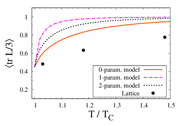
As discussed before, chooosing to be near one makes the width of the transition region narrower. In Fig. (8) we show the result for the Polyakov loop between the models with zero, one, and two parameters. The width of the transition is broadest for zero parameters, with , followed by that with two parameters, where , and then by that with one parameter, .
We also plot the results for the renormalized loop from lattice simulations. The results for the Polyakov loop in our model differ sharply from those obtained from the lattice. We do not understand the reason for this discrepancy.
Lastly, we show the results for the Polyakov loop, in our model, from different numbers of colors in Fig. (9). They differ near , below , but above this temperature, they are all rather close to one another. This is what one expects from the conformal anomaly, which up to an overall factor of , scales similarly for all .

V Interface tensions
An interface tension is computed as follows. Put the system in a box which is long in one spatial direction, say the direction. Let the system be in one vacuum at one end of the box, and a degenerate but inequivalent vacuum at the other end of the box. The theory is in a vacuum state at both ends, but not in between, so forming this interface costs action. This action is proportional to the transverse volume, , with the coefficient defined to be the interface tension.
Above , one can have the theory in one vacua at one end of the box, and a different vacua at the other. This is known as the order-order interface tension. It is equivalent to a ’t Hooft loop in the deconfined phase [74, *KorthalsAltes:2000gs]. We only compute here for two and three colors, where there is only one ’t Hooft loop. For four or more colors, there is more than one ’t Hooft loop, which we comment upon in the Conclusions, Sec. (IX).
If the transition is of first order, as it is for , then precisely at , the confined vacuum, with , is degenerate with the deconfined state, at . This can then be used to define the order-disorder interface tension.
The computation of interface tensions in the semi-QGP is close, but not identical, to that in the perturbative QGP [62, *Bhattacharya:1992qb, 64, *Giovannangeli:2004sg]. In the effective action , in addition to the potential we need a kinetic term,
| (104) |
In general, the kinetic term can be of the form
| (105) |
where is a “metric” depending on . Such a nontrivial metric arises in computing interface tensions at next to leading order in the coupling constant [63, 64, *Giovannangeli:2004sg]
At leading order, however, we can use the form of the kinetic term at tree level,
| (106) |
We have assumed that is a function only of the long spatial direction, , of the interface.
Assume that the vacua at the two ends of the box, and , are and . These correspond to the two minima, and . We take the spatial length .
The interface tension is related to the shortest path between and . This path obeys the following equation of motion
| (107) |
with the boundary condition and . Multiplying , and integrating over , we obtain an “energy” density,
| (108) |
This quantity is independent of , so its value can be taken from either end. The kinetic term does not contribute at , so the energy is given by the potential in vacuum, .
Using the conservation of “energy”, we define
| (109) |
The effective action becomes
| (110) |
where .
The interface tension is then
| (111) |
This is a general form of the interface tension. The potential depends upon the problem at hand.
V.1 The order-disorder interface tension under the uniform eigenvalue ansatz
The order disorder interface is the simplest to consider. We work at the critical temperature, so we are tunneling from the deconfined state at , to the confined vacuum, at , and compute under the uniform eigenvalue ansatz.
From Eqs. (20) and (61), the kinetic term becomes
| (112) |
where we now allow to be a function of the spatial direction .
At the critical temperature, the potential is
| (113) |
where the potential is given by Eq. (79). We now rescale the coordinate as
| (114) |
so the action becomes
| (115) |
Using the conservation of “energy”, the integral becomes
| (116) |
where is given in Eq. (78). Using this value, the order disorder interface tension is given by
| (117) |
As for the order-order interface tension, this is proportional not to , but to , because the potential for is generated at one loop order. It is proportional to at large , which is typical of the free energy in the deconfined phase.
To compare to the lattice, we need to assume a value for the coupling. We take , simply to get an idea of the numbers, and in particular, of the -dependence.
On the lattice, there are results for three colors by Beinlich, Peikert, and Karsch [12] and by Lucini, Teper, and Wenger [16]. For four or more colors, there are results from Ref. [16].
We summarize the comparsion for order-disorder interface tension, , in the following table:
| (118) |
Taken at face value, the values of the order-disorder interface tension computed in the two parameter model agree remarkably well with those from the lattice.
This agreement could well be fortuitous. We have only included the result to leading order in the coupling constant, . For the order-disorder interface tension, it is known that including at least corrections to [63], and to [64, 65] are essential to obtain agreement with lattice results, even at temperatures , well into the perturbative QGP [76].
Even so, the fit to the latent heat indicates a lower value of in the two parameter model than in the one parameter model, Eq. (103). Because of the overall factor of in the order-disorder interface tension, Eq. (117), the results do support a value of which decreases as increases.
We conclude this section with a general comment. While the order-disorder interface tension is of order at large , in fact the coefficient, from either lattice simulations or our two parameter model, is extremely small, .
This is in sharp contrast to the latent heat, which is, properly normalized, a number of order one. For an ideal gas of gluons, the energy density is times a pure number, . At infinite , by Eq. (100) the energy density at is times ; thus the latent heat is almost the energy density of an ideal gas. This is well known from three colors: the energy density very quickly approaches that of an ideal gas, close to .
Our model provides a qualitative explanation for why the latent heat is large, but the order-disorder interface tension is small. The latent heat is given by the “jump” in the order parameter, essentially by . For any , this is not a small number; at infinite , , Eq. (80). Note that since is a number between and , we can speak of its magnitude without qualification.
In contrast, the order-disorder interface tension is given by the probability for tunneling through the barrier at . Even if the jump in is large, the probability not to tunnel through the barrier can be small, if the height of the barrier is very small. That is, it is a shallow potential.
Such a shallow potential is exhibited by our model. For simplicity, consider the potential at infinite . At the critical temperature, by Eq. (79) the potential is
| (119) |
The confined vacuum is at , while at , the deconfined vacuum is at . Between and , the maximum occurs at . At this maximum, the value of the potential is . This is certainly a barrier, but to gauge its height, consider the value of the potential at the perturbative vacuum, , which is . That is, the potential at the maximum of the barrier is smaller by a factor of than what might have been expected. This is why the order-disorder interface tension is so much smaller than expected, because it is a broad, but very shallow, potential in .
Needless to say, this also illustrates the virtue of computing quantities, such as the order-disorder interface tension: it gives one insight into more detailed properties of the theory than available from just bulk thermodynamics.
V.2 The order-order interface tension for two colors
We next turn to the order-order interface tension, or ’t Hooft loop, for two colors. This is simple because there is only one direction in the Weyl chamber, along the Pauli matrix . Thus moving to a confining phase, or tunneling from one vacua to another, occurs along the same direction. This greatly simplifies the computation, and allows us to compute analytically, as in the previous section.
For two colors, one can show from Eq. (73) that the potential for has a simple form,
| (120) |
The value of the potential at , , enters only into the vacuum energy, , and can be ignored.
This potential behaves as expected: the mass for vanishes at , so the transition is of second order. In the deconfined phase, , there are two degenerate vacua, at . The represents the two degenerate vacua in the theory. At a given , we want to determine the tunneling probability between the and .
The kinetic term is as in Eq. (112). We rescale the position as
| (121) |
so that the action becomes
| (122) |
By changing , the potential, and the related integral, is precisely that of the previous section. The result for the order-order interface tension is
| (123) |
remember .
As , the order-order interface tension vanishes, as . By universality, this interface tension should vanish as , where ; lattice results by de Forcrand, D’Elia, and Pepe [77] find . Our result is a type of mean field theory, though, and so we certainly do not expect our result to correctly describe the critical region, which is very near .
V.3 The order-order interface tension for three colors
For three colors, the path to the confined vacuum is along the direction, while that for the ’t Hooft loop is along the direction in Fig. (10). Thus we have to determine a path in two dimensions. This problem can be solved numerically, but is not amenable to analytic solution.
We choose a vacuum in the semi-QGP as .
| (124) |
We wish to find a path which tunnels from this point to a transform of this point, ,
| (125) |
We parameterize this path as
| (126) |
The potential which governs this tunneling is
| (127) |
where
| (128) |
Without loss of generality, we can choose the variables to satisfy , , and . The potential becomes
| (129) |
where corresponds to .
The kinetic term is
| (130) |
where .
The interface tension becomes
| (131) |
where .
For two colors, the path is in one direction, and so we can use energy conservation to determine the action to tunnel, even without an explicit form of the solution. For three colors, the path is in two directions, and so energy conservation does not, by itself, determine the solution, nor its action.
Thus we need to explicit determine the path which tunnels between the two degenerate vacua. This satisfies the equation of motion,
| (132) |
The boundary conditions which the solution obeys is
| (133) |
These boundary conditions do not uniquely determine the solution, because we need to specify the turning point. We require that the turning point occurs at the middle of the interface, , so that
| (134) |
This is natural, since the potential is symmetric under . This also implies that at the turning point,
| (135) |
At this point, the derivative of is obtained by energy conservation, Eq. (109):
| (136) |
In the numerical computations, we use Eq. (136) as a boundary condition instead of Eq. (133).
In the perturbative QGP, is the vacuum, so that as , the derivative vanishes at . In this case, the path with a straight line is the solution of the equation of motion. This is a path along [62, 63].
In the semi-QGP, the straight line is no longer the solution of the equation of motion. That is, the path is along both and . In this case, it is necessary to solve the equations numerically.
In Fig. (10) we show the path in the plane of and . This shows that as approaches , the tunnelling path passes closer and closer to the confining vacuum, where both and vanish. For three colors, the fact that is small at in the middle of the interface has been observed previously within a Polyakov loop model [61]. We also note that the interface tension has been analyzed in linear models [48, *deForcrand:2008a, *Zhang:2011aa].
In Fig. (11), we give the result for the order-order interface tension, . We remark that while in principle for all temperatures, in practice this is very small except close to . This means that to a good approximation, we can take a path along when . We also note that in plotting the interface tension in our model, versus that from the lattice [78], that we have included a perturbative correction . This correction was computed in the perturbative QGP, and so should be recomputed for the semi-QGP. Except for , however, it can be shown that this correction is correct [79].


We conclude by discussing the problem of order-order interface tensions for four or more colors. In the complete QGP, the path for order-order interface tension is along one of the hypercharge directions, the of Eq. (43) [64, 65]. The example of three colors shows, however, that near , one will have to compute a path in the full space of dimensions. This is an interesting but nontrivial exercise in minimization, which we defer for now. We comment further about these interface tensions in the Conclusions, Sec. (IX).
VI Numerical solution of the model for four to seven colors
Before describing our numerical results, we first make an elementary but useful remark. As discussed preceeding Eq. (60), by a global rotation we can require that the expectation value of the Polyakov loop is real. If or , this means that the solution involves degrees of freedom. At infinitely high temperature all ’s vanish. As the temperature decreases the ’s move along a curve in this -dimensional space, until at the critical temperature they end up at a point . At this point, the value of the potential equals that in the confined vacuum, where , Eq. (47). This assumes that the transition is of first order, so that ; we justify this later in Sec. (VII).
For finite , the path in the -dimensional space can be determined numerically. The total potential in our model is given by
| (137) |
We have chosen very specific forms for the functions , , and , but the following conclusion is independent of their specific form.
The solution of the model at a given temperature, , is given by requiring that the total potential is stationary with respect to the ’s,
| (138) |
which is the generalization of Eq. (74).
Because the -dependence only enters through two functions, and , trivially this equation only involves only the ratio . Whatever the specific form of these two functions, at a given temperature this is a pure number.
This implies that in the -dimensional space of the ’s, that the path is independent of the choice of these two functions. Further, it follows immediately that the endpoint of the path, , is also independent of this choice of these two functions.
That the endpoint is independent of these functions was observed previously for the uniform eigenvalue ansatz. There, it was found that the properties of the solution at were independent of the one, free parameter, .
Needless to say, different choices of the functions do give different physics. While the path in -space is independent of the ’s, thermodynamic quantities also involve derivatives with respect to temperature, and these change as and do. That is, the temperature dependence of how one proceeds along this fixed path depends upon the choice of these functions. In the uniform eigenvalue ansatz, this is what changing the parameter does: it shifts the overall scale of in a nonlinear fashion.

VI.1 Four and five colors
We now turn to the case of four colors. In Fig. (12) we illustrate the region of the Weyl chamber in which the expectation value of the Polyakov loop is real. This is the plane spanned by the hypercharge and by .
The confining vacuum is given by the barycenter, . The curves where vanish, for , , and , are also indicated. The uniform eigenvalue ansatz is the line . In this ansatz, the point is given by a blue point; that for the exact solution is given by a magenta cross.
Under a transformation, the triangle maps onto itself: and interchange with one another, while the lines where vanish are left invariant.
The numerical solution for the trajectory of is plotted in Fig. (13). There are two positive eigenvalues, and . In the uniform eigenvalue ansatz, . The left panel shows the path in the plane of and ; visually, this is obviously very close to a straight line. The left panel shows the values of and ; the amount by which indicates the deviation from the uniform eigenvalue ansatz. Even at , this deviation is very small. As discussed previously, for thermodynamic quantities, and the expectation value of the Polyakov loop, the results are within the width of the curves in Figs. (5) and (9), respectively.
In spin systems there is a possibility to have mixed phases between ordered and disordered phases where is broken but is unbroken. For such a invariant phase would have and . For example, the point along this line where is indicated by the point . We find no evidence for such a phase at any temperature. This agrees with numerical simulations on the lattice [80] .


For five colors the plane where the Polyakov loop is real is shown in Fig. (14); it is spanned by the line and . In this plane is real and we expect the trajectory of the minima to again nearly coincide with the straight line ansatz from the origin to , as for four colors. This is indeed the case as is evident from Fig. (15). Only near do the eigenvalues of the Wilson line deviate from the straight line. Here, too, we found that the thermodynamic functions with those obtained above with the straight line ansatz.


VI.2 Six and seven colors
In this case the space where the Polyakov loop is real is three dimensional.
For six colors we find again that the exact solution is close to that of the uniform eigenvalue ansatz. It is also possible to have intermediate phases in which there is a global or symmetry. We find no evidence of such partially deconfined phases.
We comment that the symplectic group is the pseudo-real part of ; by exhanging the short and long roots of , this is th dual of [81]. As already remarked in section (III), to one loop order the perturbative potentials are therefore related by duality. If the non-perturbative potentials are assumed to be dual as well, then the deconfining phase transitions are the same [68]. This can be tested through numerical simulations on the lattice.
In Fig. (17) we show the path for the exact solution. In the uniform eigenvalue ansatz, . We find that the deviation from this is small except close to . The results for seven colors are interesting because of their relevance for the confining states in and groups, discussed in Sec. (VIII).


VII Why the deconfining phase transition is of first order for four or more colors
In this section we discuss why a first order transition is expected generically in matrix models when .
We first review the standard argument for why the transition is of first order for three colors [39]. If is the loop in the fundamental represetation, we consider a general potential invariant under transformations,
| (139) |
The corresponding potential includes two terms. First, there is
| (140) |
which is invariant under transformations. Second, there is
| (141) |
which is invariant only under .
For three colors, Eq. (141) is a cubic invariant, and is, in the sense of the renormalization group, a relevant operator. By standard mean field analysis, the transition is of first order. We note that there is a qualification: if the coupling vanishes, then the transition could be of second order (if ). There is no symmetry reason why should vanish, though, and so one expects a first order transition.
For four colors, Eq. (141) is a quartic term, and so marginal. For five or more colors, it is of pentic or higher order, and so an irrelevant operator. Then the deconfining transition is of second order when , and of first order . In the latter case, a positive term stabilizes the potential.
Why, then, is the deconfining transition of first order for any ? This follows in mean field theory from a matrix model. From Eq. (73) of Sec. (III), in our particular model there is a cubic term in about the confining vacuum, . As discussed there, in mean field theory this implies that the deconfining transition is of first order.
To see that this is not an accident, consider the general form of an effective potential. We express our matrix model in terms of the , and then , but in general we can construct any function of the as a series in powers of , , and so on, up to . Each term must be invariant under transformations, so the simplest possible terms include
| (142) |
There is clearly an infinite series of such terms. The first three terms are invariant under ; the last, under . This multiplicity of terms is in contrast to a loop model, which only involves powers of the loop in the fundamental representation, .
Now we perform an elementary computation. Take the basic ansatz for , Eq. (20). We do not assume the uniform eigenvalue ansatz, Eq. (60), but consider a general path, parametrized as
| (143) |
The confined vacuum is . For the straight line path, , but this parametrization is convenient, so that the expansion in Eq. (144) has a simple form.
We can then easily compute the expansion of these quantities about the confining vacuum. We introduce and ,
| (144) |
All of these loops vanish in the confined vacuum, ; as the confined vacuum is the barycenter of the Weyl chamber, the terms linear in and do as well, Sec. (III.3). These loops then begin with terms quadratic in and . What is of relevance here is the existence of terms cubic in and , which are always .
The general pattern is clear. For most terms, such as and , etc., have terms cubic in and . This is true for any term which involves , for odd . Thus, if there are any such terms in the effective potential, then in mean field theory the transition is of first order. Note that having two fields doesn’t alter the conclusion: the point is that one cannot obtained a “flat” potential, typical of a second order transition. The variables and are useful because then the quadratic terms are diagonal.
Note that in a loop model, terms such as are even in , and do not give a first order transition. A first order transition only follows in a matrix model, where one expands about the barycenter of the Weyl chamber.
As illustrated by Eq. (144), if a term only involves , for even , then there is no term cubic in and , and the transition can be of second order. This does not invalidate the expectation of a first order transition. If the effective Lagrangian involves only even powers of , then the global symmetry of the theory is not , but . The global symmetry is then not like that expected for four colors, but for two colors, where the transition is of second order. However, as for the analysis of three colors in a loop model, there is no reason to expect such an accidental symmetry to occur. Indeed, for this to happen in a matrix model, an infinite number of terms would have to vanish.
The above analysis can be generalized for any . In general, there are cubic terms in the expansion of , except for those and where there may be a residual symmetry in , as for and .
Why the deconfining phase transition is of first order for can also be understood geometrically from the Weyl chamber for three and four colors in Fig. (2).
For three colors the Weyl chamber is an equilateral triangle, bounded by the vectors and . The confined vacuum, , is the barycenter of this triangle. The path from the perturbative vacuum, to the confined vacuum, is a straight line, .
Consider expanding an effective potential about , along this straight line. Even without computation, it is evident that the region to the right is smaller than that to the left. Thus if we expand in , where is the confined vacuum, we would expect terms of cubic order, and so a first order transition.
For four colors, instead of considering the full three dimensional space of the Weyl chamber, we can limit ourselves to the plane where the Polyakov loop is real, Fig. (12). Now the path from the perturbative vacuum to the confined vacuum is not a straight line, , but slightly bent. This is irrelevant, though: the point is that if we expand any effective potential about , simply from the shape of the Weyl chamber, it is clearly not symmetric in any manner. Thus we expect the expansion of an effective potential, about , to expand the lack of such symmetry. This is the reason for the cubic terms in Eq. (144).
The same argument applies for higher . When , the part of the Weyl chamber in which the Polyakov loop is real is -dimensional, and so it becomes more difficult to draw. Even so, the lack of symmetry about the confined vacuum for six colors can also be seen from Fig. (16).
VIII A gauge group and the law of maximal eigenvalue repulsion
VIII.1 Motivation
For groups the Polyakov loop vanishes below and there is a strict definition of the deconfining transition temperature. That the Polyakov loop vanishes is a consequence of the center of , and the associated global symmetry. The confined vacuum, , is also the point where there is maximal repulsion of the eigenvalues, Eq. (III.3). We shall see in this section that it may be more useful to think of confinement as arising not from the center symmetry per se, but from eigenvalue repulsion.
To this end, we consider groups without a center. Such groups have been considered before, starting with [82, 83, 84]. The group and it has as a two-fold covering group. Consequently, the first homotopy group is nontrivial, . This is true for all groups: they have a two-fold covering representation, , which has a center of , and are doubly connected.
Like the odd dimensional rotation groups, has a trivial center. Unlike groups, though, is simply connected. For this reason, it is especially interesting to consider [82, 83, 40, 42, 41, 81, 84]. In fact, is a subgroup of . This means that the eight dimensional spin representation of has no subgroup which corresponds to a two-fold covering of .
A feature common between and is that Polyakov loops in the fundamental representation can be screened dynamically. In , two fundamentals screen each other, . In , a fundamental field, in the representation, can be screened by three adjoint fields, in the : .
For both and , then, the Polyakov loop in the fundamental representation is always screened. This is unlike , where the fundamental field cannot be screened by the symmetry. It appears similar to with dynamical, light quarks. Consequently, we might expect there is no deconfining phase transition, but perhaps just a cross-over.
Nevertheless, lattice simulations for the group find that there appears to be a first order transition [40, 41, 42, 43, 44, *Wellegehausen:2010ai, *Wellegehausen:2011sc, 47]. Even more strikingly, the expectation value of the Polyakov loop in the fundamental representation appears to be very small below the temperature for this first order transition. Thus we are led to consider how to construct effective potentials which give confinement, and a deconfining phase transition, in the absence of any center symmetry.
The simplest approach was suggested following Eq. (22). For , the perturbative potential is a power series in the adjoint loop. The symmetry allows arbitrary powers of the neutral adjoint loop to appear, but forbids terms linear in the fundamental loop. Since has no center symmetry, though, in the nonperturbative potential there is nothing to forbid us from adding a term a term where in Eq. (22) we sum over powers of the fundamental loop, the . If the coefficient of such a term is large and of the right sign, one can drive the theory to the confined phase at low temperatures.
Another approach is to observe that . This implies that we can construct a non-perturbative potential from both and potentials. Of course we must restrict the potentials to the two dimensional Cartan space of . An easy exercise shows the confining vacuum for , , lies lies in the Cartan space of . Thus by carefully adjusting the parameters of the potential, we can ensure that the system lies in the confining vacuum below . Confinement in then forces the loop in to vanish as well.
In both cases, even without center symmetry we are adding terms to the nonperturbative potential which generate an expectation value for the fundamental loop which is either small or vanishing in the low temperature phase. Confinement is thus driven not by the center symmetry, but through the complete repulsion of eigenvalues.
The crucial question is whether the Weyl invariance of is respected by such potentials. The following simple argument is suggestive. The Weyl group of is the permutation group . The Weyl group of is , the group of rotations and reflections that leave the three dimensional cube invariant; it is of order . The Weyl group of is , the dihedral group of order . Now the latter two can be written as semi-direct products of with , respectively . This shows they are subgroups of . So the answer to the question is yes, if one neglects the fact that acts in the six dimensional Cartan space of , whereas acts in the two dimensional Cartan space of .
In Sec. (VIII.2) we discuss the three dimensional Cartan space of , the embedded Cartan space of , and their roots. Sec. (VIII.3) constructs confining potentials for both and . In Sec. (VIII.4) we give a simple proof that the type potential respects the necessary Weyl symmetry. Finally, in Sec. (VIII.5) we give results for the possible thermodynamic behavior of on the basis of some representative models.
VIII.2 The root systems of
We start with some basic facts and notation. The Polyakov loop for is , where
| (145) |
As an element of , this is a tracless matrix,
| (146) |
and defines the six dimensional Cartan space of .
has the subgroup . The Cartan space of is three dimensional, where the ’s obey three extra constraints,
| (147) |
Note that these constraints are identical to those which ensure that the trace of the fundamental loop in is real, as illustrated in Fig. (16).
is a subgroup of . Its Cartan subspace obeys one more constraint:
| (148) |
We write the corresponding matrix as , and has two degrees of freedom, appropriate to the Cartan space of .

In Fig. (18) we show the three dimensional root system of , and its subgroup. Here the basis vector corresponding to are . This figure also illustrated the restriction to the plane, where . From this figure, and standard group theory [72], the roots are given by
| (149) |
together with the six roots with opposite sign.
Clearly the twelve roots lie on the edges of the cube, and the six roots on the vertices of the octahedron. The Weyl group of this system is , the group of rotations and reflections that leave the cube and the octahedron invariant. Its order is . The group of rotations is identical to the permutation group of the four diagonal body axes of the cube.
The plane defined by contains the six like roots , to wit:
| (150) |
These are part of the root system. Then there are the six orthogonal projections of the short roots in onto the plane . The resulting projections are denoted by in Fig. (18). Below we write them as to avoid confusion with the corresponding roots :
| (151) |
The roots are indeed shorter then the like roots , as behooves the root system of . Note that the hypercharge matrices and their permutations are generating the roots, in the same way as the matrices generate the roots.
As in Eq. (36) we define
| (152) |
In the perturbative effective potential, Eq. (35), the short and long roots of appear as and . These arguments are easily found from Eqs. (150) and (151). They are, with the condition :
| (153) |
| (154) |
The root lattice of , and its Weyl chamber, are illustrated in Fig. (19). The left panel is the root lattice, with six long and six short roots. The Weyl group is generated by the two mirrors indicated in the left panel, at an angle of . The product of the two reflections is a rotation over . The group is generated by this six fold rotation and by one of the reflections. This gives the dihedral group of order , and so twelve Weyl chambers. These are shown in the right hand panel. We pick the Weyl chamber as defined by the points , and and . This is the upper half of the Weyl chamber of in fig. (2). We also indicate the confining vacuum for , ; the confining vacuum for , , and by a black curve, the path where trace of the fundamental loop in vanishes. The Weyl chamber for is precisely half that of , Fig. (2).

VIII.3 Confining potentials for and
We drop an overall factor of from the potential, and split it into perturbative and nonperturbative parts,
| (155) |
As discussed in Sec. (III) the perturbative potential is
| (156) |
where , and
| (157) |
with the roots and those of .
We now consider the types of nonperturbative potentials which can produce a confined phase at low temperature.
The first method is to take a sum as in Eq. (22), but sum over powers of the Wilson line in the fundamental representation, the . The weights of the are precisely the six from Eq. (154). This gives the potential
| (158) |
The second method is to add potentials from . We construct the nonperturbative potential to eliminate the contribution of the perturbative term at the transition temperature, .
| (159) | |||||
The potentials are defined by summing the corresponding Bernoulli polynomials over the roots of :
| (160) |
By appropriately adjusting the coefficients in the nonperturbative potential, we show that we can ensure that at the critical temperature, the system goes into the confining vacuum . We stress there is no elegance in our approach: we are manifestly constructing a confined vacuum by hand. Nevertheless, our model gives testable predictions, as shown in Sec. (VIII.5).
Along these same lines we can also construct a potential which generates confinement in : the perturbative potential is that for , while in the like potential, Eq. (160), we change the argument to . Doing this gives:
| (161) |
where
| (162) |
and
| (163) |
with the roots and those of . The like potentials are
| (164) |
As discussed following Eq. (39), perturbatively the -potentials for and are related by duality. If one generates maximal eigenvalue repulsion for , however, one obtains confinement appropriate to , while Eq. (164) for gives confinement like that of . If the law of maximal eigenvalue repulsion holds, then, the nonperturbative potentials are not related by duality [68].
VIII.4 Weyl symmetry of like potentials
In this subsection we show that the nonperturbative potentials introduced above are invariant under the Weyl symmetries of and . First observe the only terms which are not manifestly Weyl invariant are those in Eqs. (160) and (164).
Now use Eq. (154) to rewrite this in terms of the roots of roots. This gives:
| (166) |
which is manifestly invariant under the Weyl symmetry of .
Applying the same method to gives
| (167) |
Note that the constraint is absent for . Imposing it gives the result, Eq. (165). Using Eqs. (37) and (38) this can be rewritten as
| (168) |
This result is manifestly Weyl invariant as the sums are separately invariant: the Weyl transformations are orthogonal, and so cannot transform roots into roots.
VIII.5 Results for
In this section, we give results for the thermodynamics, assuming parameters which give a confined low temperature phase. The total potential is
| (169) |
where the perturbative potential is
| (170) |
For clarity, we write all functions in terms of the two independent ’s for , and . The potentials are
| (171) | |||||
We consider a nonperturbative potential
| (172) | |||||
The potentials are
| (173) | |||||
while the potential from summing over Eq. (22) using the fundamental representation, the , is
| (174) |
Besides thermodynamic quantities, such as the pressure and the interaction measure, it is also possible to measure loops. In , the fundamental representation is related to the embedding as [40], so that the fundamental loop is given by [44, *Wellegehausen:2010ai, *Wellegehausen:2011sc]
| (175) |
The adjoint representation is related to the embedding as , so that [44, *Wellegehausen:2010ai, *Wellegehausen:2011sc]
| (176) | |||||
In Eq. (172) we have a model with six parameters. Even imposing two conditions — that the transition occur at , and that the pressure vanishes there — we are left with four free parameters.
Instead of investigating the entire four dimensional space, we consider some representative models.
The first is a minimal model,
| (177) |
This is the analogy of the analogue of zero parameter model of Ref. [1]. We introduce terms to drive the theory to a Higgs phase. We could also introduce a term , which would be like our one parameter model [3]. We have done so, and find that the results are similar to the minimal model of Eq. (177).
The next is a model with a single fundamental loop,
| (178) |
The specific parameters chosen were and ; the values of and follow as for , Sec. (IV), and are and .
Finally, we consider a type model,
| (179) |
Notice that we have fixed the parameter ; with this value, the part of the nonperturbative potential cancels, identically, the perturbative potential at . This ensures that the confining effects of the potential are maximized at . We then considered two representative values of : , for which , and ; and , for which and .
In Fig. (20) show the expectation value of the Polyakov loops in the fundamental representations. At present, there is only data on histograms for the expectation value for the bare, fundamental loop [40, 41, 42, 43, 44, *Wellegehausen:2010ai, *Wellegehausen:2011sc, 47]. This shows the expectation value of the bare loop is very small in the low temperature phase. Including renormalization should not alter this conclusion. Presumably, more careful lattice studies will show that the expectation value is small, but nonzero, as true for the adjoint loop in in the confined phase [37].
Nevertheless, the minimal model appears to be excluded. It is negative at , with a value . In Fig. (21) we illustrate the Weyl chamber for , indicating both the vacua at and . The low temperature phase at is close, but not coincident with , the confining vacuum for .
The other models give fundamental loops which are small in the low temperature phase. In the fundamental loop model, this expectation value is at , which may be compatible with the lattice results. Lastly, the models automatically give zero fundamental loop below .
In Fig. (22) we give the expectation value of the adjoint loop. This also provides a way of distinguishing between different models. On the lattice, the bare adjoint loop is strongly suppressed, but with effort can be measured. In the minimal model, it is positive at , but then becomes negative. It is negative in the low temperature phase for the fundamental loop model, and essentially zero in the model.


Fig. (23) shows the evolution of the eigenvalues of the fundamental Polyakov loop with temperature for the minimal model, Eq. (177), and for the model, Eq. (179), with . We find that they remain close to although not exactly on the SU(7) path .

In Fig. (24) we show the pressure obtained from the four models, Eqs. (177), (178), and (179). This shows that the pressure itself is not very useful for differentiating between models. The pressure of the minimal model is negative below , but this is a limitation of our assumption that the pressure vanishes at .

In Fig. (25) we show the interaction measure obtained from the models. All of the transitions are of first order. The minimal model looks most like that of , with a large latent heat and a sharp peak in near . The fundamental loop model also has a sharp peak in , but its latent heat is small. Notice also that for the fundamental loop model, the expectation of the fundamental and adjoint loops, Figs. (20) and (22), is much smaller than the other models. This suggests that the fundamental loop model may be near a critical endpoint.
For the two models, the interaction measure does not exhibit a peak near , but instead drops rather slowly as the temperature increases.

Lastly, in fig. (26) we show the rescaled interaction measure, , for the four different models. That for the minimal and the fundamental loop models are flat, while that for the model is not.

IX Conclusions
In this paper we generalized the model of Ref. [1] and [3] to a theory with two parameters. The two parameters were chosen by comparing to the interaction measure. We then obtain results for the ’t Hooft loop, or the order-order interface tension, and for the order-disorder interface tension at . While for most quantities the agreement is good, within or so.
There is one glaring problem with the model: the results for the Polyakov loop, Figs. (3) and (9), look nothing like the lattice results, Refs. [37] and [38]. The discrepancy is not minor: on the lattice, the renormalized loop indicates a broad semi-QGP, from to at least . In our model, the width is extremely narrow, to only . Further, latest lattice measurements compute the renormalized loop by explicit subtraction of the zero point energy at zero temperature, which is theoretically an unambiguous proceedure.
Can corrections to our model change this? These are of two types. One is corrections in the coupling constant. For example, there are corrections to to the perturbative potential. It would also be possible to compute corrections to our potential, which includes both perturbative and non-perturbative terms. (We ignore obvious questions of principle, namely, to what extent does the non-perturbative potential include perturbative corrections?) At next to leading order, it is known that the ’s shift by an amount , [63], and the same happens in our effective model [79]. Such a shift is , and should be relatively small. More to the point, however, in our model the width of the transition region in the ’s is tied intimately to the width of the interaction measure. No matter how the ’s shift, it would seem unavoidable that the width will broaden greatly, and still give the same sharp peak in the interaction measure.
Other corrections are those . From lattice measurements, though, the behavior found for three colors [37] is very similar for four and five colors [38]. While the value of the Polyakov loop at the critical temperature changes modestly with , in all cases the transition region, as seen from the renormalized Polyakov loop, remains broad.
This discrepancy must be considered the outstanding problem in the model. We can only suggest that the effects of the non-perturbative potential broaden what is measured as the (renormalized) Polyakov loop, although the width of the transition remains narrow. For example, for three [37, 85], as well as for four and five colors [38], there are terms in the logarithm of the Polyakov loop. Perhaps there is some non-perturbative term which broadens the measured value of the Polyakov loop, but not the width of the transition region for the ’s?
We conclude by pointing out that there are two others ways in which the width of the transition region can be measured, although indirectly. One was discussed previously [3]. When the ’s develop an expectation value, the theory is an adjoint Higgs phase. In our model, in principle this happens for all , but in practice it is only numerically large below . While there is no order parameter to distinguish such an adjoint Higgs phase, it generates a characteristic splitting of masses. One may have to work very close to to see this, but it is a necessary consequence of our model.
The ’t Hooft loop provides another way of testing a narrow transition region. In Sec. (V) we gave results for the ’t Hooft loop in the semi-QGP. Better measurements of these quantities should provide a stringent test of our model.
For four or more colors, there are further tests. For four colors, besides the simplest ’t Hooft loop, between a Polyakov loop with phase and , there is also a loop between and . To , the ratio of these ’t Hooft loops satisfy Casimir scaling [64, *Giovannangeli:2004sg]. This Casimir scaling is observed to a very good precision over a wide range in temperature [78]. We have not computed the ratio of these ’t Hooft loops in our model, but suggest that it will produce small, but measureable deviations from Casimir scaling in the ratio of such ’t Hooft loops, certainly in the region close to , for .
In conclusion, we suggest that detailed measurements of the pure glue theory, especially near , can help illuminate how the law of maximal eigenvalue repulsion acts to generate confinement.
Acknowledgements.
The research of A.D. was supported by the U.S. Department of Energy under contract #DE-FG02-09ER41620, and by PSC-CUNY research grant 64132-00 42; of Y.H. by a Grant-in-Aid for Scientific Research (No.23340067) from the Ministry of Education, Culture, Sports, Science and Technology (MEXT) of Japan; of R.D.P., by the U.S. Department of Energy under contract #DE-AC02-98CH10886. C.P.K.A. thanks the Nuclear Theory Group at BNL for their warm hospitality. We thank T. Umeda and the WHOT collaboration for sharing their data with us [13], which enabled us to plot Fig. (1). R.D.P. thanks J. Pawlowski for numerous discussions on the model of Ref. [51], which also exhibits a narrow transition region; V. Begun, for bringing [31] to his attention; and A. Bazavov, F. Karsch, M. Panero, and P. Petreczky for discussions. C.P.K.A. thanks Oleg Ogievetsky and Loic Poulain d’Andecy for their explanations about classical groups.References
- [1] P. N. Meisinger, T. R. Miller, and M. C. Ogilvie, Phys.Rev. D65, 034009 (2002), arXiv:hep-ph/0108009 [hep-ph] .
- [2] P. N. Meisinger and M. C. Ogilvie, Phys.Rev. D65, 056013 (2002), arXiv:hep-ph/0108026 [hep-ph] .
- [3] A. Dumitru, Y. Guo, Y. Hidaka, C. P. K. Altes, and R. D. Pisarski, Phys.Rev. D83, 034022 (2011), arXiv:1011.3820 [hep-ph] .
- [4] C. DeTar and U. Heller, Eur.Phys.J. A41, 405 (2009), arXiv:0905.2949 [hep-lat] .
- [5] P. Petreczky, (2012), arXiv:1203.5320 [hep-lat] .
- [6] J. Engels, J. Fingberg, K. Redlich, H. Satz, and M. Weber, Z.Phys. C42, 341 (1989).
- [7] J. Engels, J. Fingberg, and M. Weber, Nucl.Phys. B332, 737 (1990).
- [8] J. Engels, J. Fingberg, and D. Miller, Nucl.Phys. B387, 501 (1992).
- [9] J. Engels, F. Karsch, and K. Redlich, Nucl.Phys. B435, 295 (1995), arXiv:hep-lat/9408009 [hep-lat] .
- [10] J. Engels and T. Scheideler, Nucl.Phys. B539, 557 (1999), arXiv:hep-lat/9808057 [hep-lat] .
- [11] G. Boyd, J. Fingberg, F. Karsch, L. Karkkainen, and B. Petersson, Nucl.Phys. B376, 199 (1992).
- [12] B. Beinlich, F. Karsch, and A. Peikert, Phys.Lett. B390, 268 (1997), arXiv:hep-lat/9608141 [hep-lat] .
- [13] T. Umeda, S. Ejiri, S. Aoki, T. Hatsuda, K. Kanaya, et al., Phys.Rev. D79, 051501 (2009), arXiv:0809.2842 [hep-lat] .
- [14] S. Borsanyi, G. Endrodi, Z. Fodor, S. Katz, and K. Szabo, (2012), arXiv:1204.6184 [hep-lat] .
- [15] B. Lucini, M. Teper, and U. Wenger, JHEP 0401, 061 (2004), arXiv:hep-lat/0307017 [hep-lat] .
- [16] B. Lucini, M. Teper, and U. Wenger, JHEP 0502, 033 (2005), arXiv:hep-lat/0502003 [hep-lat] .
- [17] M. Teper, PoS LATTICE2008, 022 (2008), arXiv:0812.0085 [hep-lat] .
- [18] M. Panero, Phys.Rev.Lett. 103, 232001 (2009), arXiv:0907.3719 [hep-lat] .
- [19] S. Datta and S. Gupta, Phys.Rev. D82, 114505 (2010), arXiv:1006.0938 [hep-lat] .
- [20] B. Lucini, A. Rago, and E. Rinaldi, (2012), arXiv:1202.6684 [hep-lat] .
- [21] Y. Hidaka and R. D. Pisarski, Phys.Rev. D78, 071501 (2008), arXiv:0803.0453 [hep-ph] .
- [22] Y. Hidaka and R. D. Pisarski, Phys.Rev. D80, 036004 (2009a), arXiv:0906.1751 [hep-ph] .
- [23] Y. Hidaka and R. D. Pisarski, Phys.Rev. D80, 074504 (2009b), arXiv:0907.4609 [hep-ph] .
- [24] Y. Hidaka and R. D. Pisarski, Phys.Rev. D81, 076002 (2010), arXiv:0912.0940 [hep-ph] .
- [25] R. D. Pisarski, Phys.Rev. D62, 111501 (2000), arXiv:hep-ph/0006205 [hep-ph] .
- [26] A. Dumitru, Y. Hatta, J. Lenaghan, K. Orginos, and R. D. Pisarski, Phys.Rev. D70, 034511 (2004), arXiv:hep-th/0311223 [hep-th] .
- [27] A. Dumitru, J. Lenaghan, and R. D. Pisarski, Phys.Rev. D71, 074004 (2005), arXiv:hep-ph/0410294 [hep-ph] .
- [28] M. Oswald and R. D. Pisarski, Phys.Rev. D74, 045029 (2006), arXiv:hep-ph/0512245 [hep-ph] .
- [29] R. D. Pisarski, Phys.Rev. D74, 121703 (2006), arXiv:hep-ph/0608242 [hep-ph] .
- [30] O. Andreev, Phys.Rev. D76, 087702 (2007), arXiv:0706.3120 [hep-ph] .
- [31] V. Begun, M. Gorenstein, and O. Mogilevsky, Int.J.Mod.Phys. E20, 1805 (2011), arXiv:1004.0953 [hep-ph] .
- [32] J. M. Cornwall, J. Papavassiliou, and D. Binosi, The Pinch Technique and Its Applications to Non-Abelian Gauge Theories (Cambridge University Press, 2011).
- [33] A. Peshier, B. Kampfer, O. Pavlenko, and G. Soff, Phys.Rev. D54, 2399 (1996).
- [34] P. Castorina, D. E. Miller, and H. Satz, Eur.Phys.J. C71, 1673 (2011), arXiv:1101.1255 [hep-ph] .
- [35] M. Caselle, L. Castagnini, A. Feo, F. Gliozzi, and M. Panero, JHEP 1106, 142 (2011a), arXiv:1105.0359 [hep-lat] .
- [36] M. Caselle, L. Castagnini, A. Feo, F. Gliozzi, U. Gursoy, et al., (2011b), arXiv:1111.0580 [hep-th] .
- [37] S. Gupta, K. Huebner, and O. Kaczmarek, Phys.Rev. D77, 034503 (2008), arXiv:0711.2251 [hep-lat] .
- [38] A. Mykkanen, M. Panero, and K. Rummukainen, (2012), arXiv:1202.2762 [hep-lat] .
- [39] B. Svetitsky and L. G. Yaffe, Nucl.Phys. B210, 423 (1982).
- [40] K. Holland, P. Minkowski, M. Pepe, and U. Wiese, Nucl.Phys.Proc.Suppl. 119, 652 (2003), arXiv:hep-lat/0209093 [hep-lat] .
- [41] M. Pepe and U.-J. Wiese, Nucl.Phys. B768, 21 (2007), arXiv:hep-lat/0610076 [hep-lat] .
- [42] G. Cossu, M. D’Elia, A. Di Giacomo, B. Lucini, and C. Pica, JHEP 0710, 100 (2007), arXiv:0709.0669 [hep-lat] .
- [43] C. Hoyos-Badajoz, B. Lucini, and A. Naqvi, JHEP 0804, 075 (2008), arXiv:0711.0659 [hep-th] .
- [44] B. H. Wellegehausen, A. Wipf, and C. Wozar, Phys.Rev. D80, 065028 (2009), arXiv:0907.1450 [hep-lat] .
- [45] B. H. Wellegehausen, A. Wipf, and C. Wozar, Phys.Rev. D83, 016001 (2011a), arXiv:1006.2305 [hep-lat] .
- [46] B. H. Wellegehausen, A. Wipf, and C. Wozar, Phys.Rev. D83, 114502 (2011b), arXiv:1102.1900 [hep-lat] .
- [47] M. Bruno, M. Caselle, M. Panero, and R. Pellegrini, (work in progress, 2012).
- [48] A. Vuorinen and L. G. Yaffe, Phys.Rev. D74, 025011 (2006), arXiv:hep-ph/0604100 [hep-ph] .
- [49] P. de Forcrand, A. Kurkela, and A. Vuorinen, Phys.Rev. D77, 125014 (2008), arXiv:0801.1566 [hep-ph] .
- [50] T. Zhang, T. Brauner, A. Kurkelna, and A. Vuorinen, (2011), arXiv:1112.2983 [hep-ph] .
- [51] J. Braun, H. Gies, and J. M. Pawlowski, Phys.Lett. B684, 262 (2010a), arXiv:0708.2413 [hep-th] .
- [52] F. Marhauser and J. M. Pawlowski, (2008), arXiv:0812.1144 [hep-ph] .
- [53] J. Braun, A. Eichhorn, H. Gies, and J. M. Pawlowski, Eur.Phys.J. C70, 689 (2010b), arXiv:1007.2619 [hep-ph] .
- [54] O. Scavenius, A. Dumitru, and J. Lenaghan, Phys.Rev. C66, 034903 (2002), arXiv:hep-ph/0201079 [hep-ph] .
- [55] K. Fukushima, Phys.Lett. B591, 277 (2004), arXiv:hep-ph/0310121 [hep-ph] .
- [56] T. Hell, S. Rossner, M. Cristoforetti, and W. Weise, Phys.Rev. D81, 074034 (2010), arXiv:0911.3510 [hep-ph] .
- [57] K. Fukushima and T. Hatsuda, Rept.Prog.Phys. 74, 014001 (2011), arXiv:1005.4814 [hep-ph] .
- [58] F. Buisseret and G. Lacroix, Phys.Rev. D85, 016009 (2012), arXiv:1107.4672 [hep-ph] .
- [59] D. Horvatic, D. Blaschke, D. Klabucar, and O. Kaczmarek, Phys.Rev. D84, 016005 (2011), arXiv:1012.2113 [hep-ph] .
- [60] T. Hell, K. Kashiwa, and W. Weise, Phys.Rev. D83, 114008 (2011), arXiv:1104.0572 [hep-ph] .
- [61] B. Layek, A. P. Mishra, and A. M. Srivastava, Phys.Rev. D71, 074015 (2005), arXiv:hep-ph/0502250 [hep-ph] .
- [62] T. Bhattacharya, A. Gocksch, C. Korthals Altes, and R. D. Pisarski, Phys.Rev.Lett. 66, 998 (1991).
- [63] T. Bhattacharya, A. Gocksch, C. Korthals Altes, and R. D. Pisarski, Nucl.Phys. B383, 497 (1992), arXiv:hep-ph/9205231 [hep-ph] .
- [64] P. Giovannangeli and C. Korthals Altes, Nucl.Phys. B721, 1 (2005a), arXiv:hep-ph/0212298 [hep-ph] .
- [65] P. Giovannangeli and C. Korthals Altes, Nucl.Phys. B721, 25 (2005b), arXiv:hep-ph/0412322 [hep-ph] .
- [66] M. Unsal and L. G. Yaffe, Phys.Rev. D78, 065035 (2008), arXiv:0803.0344 [hep-th] .
- [67] D. Simic and M. Unsal, Journal of High Energy Physics (JHEP) (2010), arXiv:1010.5515 [hep-th] .
- [68] C. Korthals Altes, (manuscript in preparation, 2012).
- [69] V. Belyaev, Phys.Lett. B254, 153 (1991).
- [70] C. Korthals Altes, Nucl.Phys. B420, 637 (1994), arXiv:hep-th/9310195 [hep-th] .
- [71] I. S. Gradshteyn and I. M. Ryzhik, Table of Integrals, Series, and Products (Academic Press, New York, 1980).
- [72] H. Georgi, Lie Algebras in Particle Physics (Westview Press, 1999).
- [73] R. D. Pisarski and V. V. Skokov, (manuscript in preparation, 2012).
- [74] C. Korthals-Altes, A. Kovner, and M. A. Stephanov, Phys.Lett. B469, 205 (1999), arXiv:hep-ph/9909516 [hep-ph] .
- [75] C. Korthals-Altes and A. Kovner, Phys.Rev. D62, 096008 (2000), arXiv:hep-ph/0004052 [hep-ph] .
- [76] P. de Forcrand and D. Noth, Phys.Rev. D72, 114501 (2005), arXiv:hep-lat/0506005 [hep-lat] .
- [77] P. de Forcrand, M. D’Elia, and M. Pepe, Phys.Rev.Lett. 86, 1438 (2001), arXiv:hep-lat/0007034 [hep-lat] .
- [78] P. de Forcrand, B. Lucini, and D. Noth, PoS LAT2005, 323 (2006), arXiv:hep-lat/0510081 [hep-lat] .
- [79] A. Dumitru, Y. Guo, N. Su, and C. Korthals Altes, “Perturbative corrections to matrix models,” (2012).
- [80] B. Lucini, M. Teper, and U. Wenger, Phys.Lett. B545, 197 (2002), arXiv:hep-lat/0206029 [hep-lat] .
- [81] K. Holland, M. Pepe, and U. Wiese, Nucl.Phys. B694, 35 (2004), arXiv:hep-lat/0312022 [hep-lat] .
- [82] K. Langfeld and H. Reinhardt, “The Stefan-Boltzmann law: SU(2) versus SO(3) lattice gauge theory,” (2000), arXiv:hep-lat/0001009 [hep-lat] .
- [83] P. de Forcrand and O. Jahn, Nucl.Phys. B651, 125 (2003), arXiv:hep-lat/0211004 [hep-lat] .
- [84] J. Greensite, K. Langfeld, S. Olejnik, H. Reinhardt, and T. Tok, Phys.Rev. D75, 034501 (2007), arXiv:hep-lat/0609050 [hep-lat] .
- [85] E. Megias, E. Ruiz Arriola, and L. Salcedo, Phys.Rev. D75, 105019 (2007), arXiv:hep-ph/0702055 [hep-ph] .