Extending partial representations of function graphs and permutation graphs
Abstract
Function graphs are graphs representable by intersections of continuous real-valued functions on the interval and are known to be exactly the complements of comparability graphs. As such they are recognizable in polynomial time. Function graphs generalize permutation graphs, which arise when all functions considered are linear.
We focus on the problem of extending partial representations, which generalizes the recognition problem. We observe that for permutation graphs an easy extension of Golumbic’s comparability graph recognition algorithm can be exploited. This approach fails for function graphs. Nevertheless, we present a polynomial-time algorithm for extending a partial representation of a graph by functions defined on the entire interval provided for some of the vertices. On the other hand, we show that if a partial representation consists of functions defined on subintervals of , then the problem of extending this representation to functions on the entire interval becomes NP-complete.
1 Introduction
Geometric representations of graphs have been studied as part of graph theory from its very beginning. Euler initiated the study of graph theory by studying planar graphs in the setting of three-dimensional polytopes. The theorem of Kuratowski [15] provides the first combinatorial characterization of planar graphs and can be considered as the start of modern graph theory.
In this paper we are interested in intersection representations, which assign geometric objects to the vertices of graphs and the edges are encoded by intersections of objects. Formally, an intersection representation of is a mapping of the vertices of to a class of objects (sets) such that if and only if . This way, for different classes we obtain various classes of representable graphs. Classic examples include interval graphs, circle graphs, permutation graphs, string graphs, convex graphs, and function graphs [9, 20]. As seen from these two monographs, geometric intersection graphs are intensively studied for their applied motivation, algorithmic properties, but also as a source of many interesting theoretical results that sometimes stimulate our curiosity (as one example we mention that string graphs requiring exponential number of crossing points in every representation are known, and yet the recognition problem is in NP).
Naturally, the recognition problem is the first one to consider. For most of the intersection defined classes the complexity of their recognition is known. For example, interval graphs can be recognized in linear time [3], while recognition of string graphs is NP-complete [13, 19]. Our goal is to study the easily recognizable classes and explore if the recognition problem becomes harder when extra conditions are given with the input.
Partial representations. A recent paper of Klavík et al. [12] introduced a question of extending partial representations for classes of intersection graphs. A partial representation of is a representation of the induced subgraph for a set . The problem of partial representation extension for a class represented in a class is defined as follows: given a graph and a partial representation of , decide whether there is a representation that extends , that is, such that .
The paper [12] investigates the complexity of the problem for intervals graphs (intersection graphs of intervals on a line) and presents an algorithm for extending interval representations and an algorithm for extending proper interval representations of graphs with vertices and edges. A recent result of Bläsius and Rutter [4] solves the problem of extending interval representations in time , but the algorithm is involved.
A related problem of simultaneous graph representations was recently introduced by Jampani and Lubiw [11]: given two graphs and sharing common vertices , decide whether there are representations of and of such that . Simultaneous representations are closely related to partial representation extension. Namely, in many cases we can solve partial representation extension by introducing an additional graph and putting . On the other hand, if is small, then we can test all essentially different possible representations of and try to extend them to and , which can give us a polynomial-time algorithm for fixed parameter .
Several other problems have been considered in which a partial solution is given and the task is to extend it. For example, every -regular bipartite graph is -edge-colorable, but if some edges are pre-colored, the extension problem becomes NP-complete even for [6], and even when the input is restricted to planar graphs [16]. For planar graphs, partial representation extension is solvable in linear time [1]. Every planar graph admits a straight-line drawing, but extending such representation is NP-complete [18].
Permutation and function graphs. In this paper, we consider two classes of intersection graphs. The class FUN of function graphs is represented by continuous monotone curves connecting two parallel lines in the plane. In other words, a representation of a function graph assigns a continuous function to every vertex of the graph. The class PERM of permutation graphs, which is a subclass of FUN, is represented the same way by linear functions.
A graph is a comparability graph if it is possible to orient its edges transitively. An orientation is transitive if and imply . Thus the relation in a transitively oriented graph is a strict partial order. We denote the class of comparability graphs by CO. A partial orientation of a comparability graph is a transitive orientation of some of its edges. The problem OrientExt is to decide whether we can orient the remaining edges to get a transitive orientation of the entire graph.
By coCO we denote the class of complements of comparability graphs. We have the following relations: [10] and [5]. We derive a transitive ordering from a function graphs as follows: if two functions do not intersect, then one is on top of the other; thus we can order the functions from bottom to top. For permutation graphs, we use the fact that .
Our results. By a straightforward modification of the recognition algorithms of Golumbic [8, 9] and by the property , we get the following.
Proposition 1
The problem OrientExt can be solved in time for graphs with vertices, edges, and maximum degree .
Proposition 2
The problem can be solved in time for graphs with vertices.
Our first main result is a polynomial-time algorithm for . Here the straightforward generalization of the recognition algorithm does not work. Even though , the problems and OrientExt are different, see Fig. 1. This is similar to what happens for the classes of proper and unit interval graphs: they are known to be equal, but their partial representation extension problems are different [12].
Theorem 1.1
The problem can be solved in polynomial time.
0,0)(86,23.2)
The second main result concerns partial representations by partial functions with , which generalize ordinary partial representations by functions. The problem is to decide, for a given graph, whether a given partial representation by partial functions can be extended to a representation of the whole graph so that all partial functions are extended to functions defined on the entire .
Theorem 1.2
The problem is NP-complete.
2 Extending partial orientation of a comparability graph
We show how to modify the recognition algorithm of Golumbic [8, 9] to obtain an algorithm for extending partial orientation of a comparability graph. The recognition algorithm repeats the following until the whole graph is oriented. We pick an arbitrary unoriented edge and orient it in any direction. This may force several other edges to be oriented, according to the following rules:
- •
and force ,
- •
, , and force .
If we find an edge that we are forced to reorient (change its direction), then we stop and answer that is not a comparability graph. Otherwise, we finally orient all edges and obtain a transitive orientation of . The running time of the algorithm is .
Now, we adapt this algorithm to the problem OrientExt. Since the algorithm processes edges in an arbitrary order, we can choose an ordering of the edges and always pick the first non-oriented edge in this ordering. Suppose that the first edges are preoriented by . If we pick an edge , then we orient it according to if or arbitrarily otherwise. The algorithm additionally fails if it is forced to orient an edge with in the opposite direction to the one forced by . In such a case, this orientation is forced by the orientation of , and thus the partial orientation is indeed not extendible. The running time of the algorithm is again , which proves Proposition 1. The detailed proof of Proposition 2 is in the Appendix.
3 Extending partial representation of a poset
Before we deal with function representations of graphs, we study representations of posets by continuous functions . By a poset we mean a transitively oriented graph. We write to denote that there is an edge from to in a poset . Since we are interested in algorithmic problems, we have to choose some discrete description of the functions, and the particular choice does not matter as long as we can convert from and to other descriptions in polynomial time. Here we restrict our attention to piecewise linear continuous functions. Specifically, each function that we consider is described by a tuple of points in with so that is linear on every interval . We denote the family of such functions by . Note that every representation by continuous functions can be approximated by an equivalent representation by functions from . We define a natural order on by setting whenever holds for every . A representation of a poset is a mapping such that
It is worth to note that every poset has a representation of this kind, see [10]. A partial representation of a poset is a mapping which is a representation of the subposet induced on a set .
In this section we provide a polynomial-time algorithm solving the following problem: given a poset and its partial representation , decide whether is extendable to a representation of . Thus for the remainder of this section we assume that is a poset, , and is a partial representation of .
For a function we define
For every vertex of we define a set , called the region of , as follows. If , then . Otherwise,
It follows that the function representing in any representation of extending must be contained entirely within . See Fig. 2 for an illustration.
0,0)(90,26)
Lemma 1
There is a representation of extending if and only if any two incomparable vertices and of satisfy .
The proof is in the Appendix.
Lemma 1 directly yields a polynomial-time algorithm for deciding whether has a representation extending . Indeed, the lower or upper boundary of (if exists) is a function from whose description can be easily computed from the descriptions of the functions with and or , respectively. Having the descriptions of the lower and upper boundaries of all regions, we can easily check whether the intersection of any two of them is empty.
4 Modular decomposition
The main tool that we use for constructing a polynomial-time algorithm for extending partial representations of function graphs is modular decomposition, also known as substitution decomposition. In this section we briefly discuss this concept and its connection to transitive orientations of graphs.
A graph is empty if it has no edges. A graph is complete if it has all possible edges. A set is a module of if every vertex in is adjacent to either all or none of the vertices in . The singleton sets and the whole are the trivial modules of . A non-empty graph is prime if it has no modules other than the trivial ones. A module is strong if every module satisfies , , or . We denote the family of non-singleton strong modules of by . A strong module is maximal if there is no strong module with . When is a graph with at least two vertices, the maximal strong modules of form a partition of , which we denote by . It is easy to see that a set is a strong module of if and only if is a strong module of for some . Applying this observation recursively, we see that the strong modules of form a rooted tree, called the modular decomposition of , in which
- •
is the root;
- •
are the children of every ;
- •
the singleton modules are the leaves.
In particular, has at most strong modules in total.
Any two distinct strong modules can be either adjacent, which means that any two vertices and are adjacent in , or non-adjacent, which means that no two vertices and are adjacent in . When and are two adjacent strong modules of and is a transitive orientation of , we write to denote that for all and .
Theorem 4.1 (Gallai [7])
Let and be two adjacent strong modules of . Every transitive orientation of satisfies either or .
For a module , we call the adjacency graph of the quotient of and denote it by , and we call a transitive orientation of simply a transitive orientation of .
Theorem 4.2 (Gallai [7])
The transitive orientations of and the tuples of transitive orientations of non-singleton strong modules of are in a one-to-one correspondence given by for any and . In particular, is a comparability graph if and only if is a comparability graph for every .
Theorem 4.3 (Gallai [7])
Let be a non-singleton strong module of .
- 1.
If is not connected, then the maximal strong modules of are the connected components of and is an empty graph.
- 2.
If is not connected, then the maximal strong modules of are the connected components of and is a complete graph.
- 3.
If and are connected, then is a prime graph.
Theorem 4.3 allows us to classify non-singleton strong modules into three types. Namely, a non-singleton strong module of is
- •
parallel when is empty;
- •
serial when is complete;
- •
prime when is prime.
Every parallel module has just one transitive orientation—there is nothing to orient in an empty quotient. Every serial module with children has exactly transitive orientations corresponding to the permutations of the children. Finally, for prime modules we have the following.
Theorem 4.4 (Gallai [7])
Every prime module of a comparability graph has exactly two transitive orientations, one being the reverse of the other.
Golumbic [8, 9] showed that the problems of computing the modular decomposition of a graph, computing the two transitive orientations of a prime comparability graph, and deciding whether a graph is a comparability graph are polynomial-time solvable. Actually, the first two of these problems can be solved in linear time [17].
5 Extending partial represenation of a function graph
In this section we provide a polynomial-time algorithm for extending partial representation of function graphs. However, for convenience, instead of function graphs we deal with their complements—comparability graphs. A representation of a comparability graph is a representation of a transitive orientation of , defined as in Section 3. A partial representation of is a representation of an induced subgraph of .
Specifically, we prove that the following problem is polynomial-time solvable: given a comparability graph and its partial representation , decide whether is extendable to a representation of . Thus for the remainder of this section we assume that is a comparability graph, , and is a partial representation of .
A transitive orientation of respects if is a partial representation of . The idea of the algorithm is to look for a transitive orientation of that respects and satisfies for any two adjacent vertices and of , where by we denote the region of with respect to . By Lemma 1, such a transitive orientation exists if and only if is extendable. We make use of the modular decomposition of and Theorem 4.2 to identify all transitive orientations of . We apply to a series of reductions, which ensure that every non-singleton strong module of has exactly one or two transitive orientations respecting , while not changing the answer. Finally, after doing all these reductions, we express the existence of a requested transitive orientation of by an instance of 2-SAT.
A strong module of is represented if . Any vertex from is a representant of . Clearly, if is represented, then all ancestors of in the modular decomposition of are represented as well.
The first step of the algorithm is to compute the modular decomposition of , which can be done in polynomial time as commented at the end of the previous section. Then, we apply three kinds of reductions, which modify and its modular decomposition but do not affect and :
- 1.
If there is a non-singleton non-represented module of , then choose any vertex , remove (with all incident edges) from and from the nodes of the modular decomposition, and replace the subtree rooted at by the singleton module in the modular decomposition.
- 2.
If there is a serial module of with two or more non-represented children, then we choose any non-represented child of and remove from and from the modular decomposition all other non-represented children of .
- 3.
If there is a serial module of with two or more represented children and some non-represented children, then we remove from and from the modular decomposition all non-represented children of .
Lemma 2
The graph has a representation extending if and only if the graph obtained from by reductions 1–3 has a representation extending .
The proof is in the Appendix.
We apply reductions 1–3 in any order until none of them is applicable any more, that is, we are left with a graph such that
- •
every non-singleton strong module of is represented,
- •
every serial module of has at most one non-represented child,
- •
every serial module of with at least two represented children has no non-represented child.
For such we have the following.
Lemma 3
Let be a non-singleton strong module of . If is
- •
a serial module with a non-represented child,
- •
a prime module with no two adjacent represented children,
then has exactly two transitive orientations, one being the reverse of the other, both respecting . Otherwise, has just one transitive orientation respecting .
The proof is in the Appendix.
Lemma 4
Let be a non-represented vertex of and be the parent of in the modular decomposition of . For transitive orientations of respecting , the set is determined only by the transitive orientation of induced by .
Proof
Let be a represented vertex of adjacent to . We show that the orientation of the edge either is the same for all transitive orientations of respecting or depends only on the transitive orientation of . This suffices for the conclusion of the lemma, as the set is determined by the orientations of edges connecting with represented vertices of .
If , then clearly the orientation of the edge depends only on the transitive orientation of . Thus suppose . Let be a representant of . Since is a module, is adjacent to as well. By Theorem 4.1, the orientations of the edges and are the same for every transitive orientation of . The orientation of and thus of in any transitive orientation of respecting is fixed by . Therefore, all transitive orientations of respecting yield the same orientation of the edge .∎
By Lemmas 3 and 4, for every , all transitive orientations of respecting yield at most two different regions . We can compute them following the argument in the proof of Lemma 4. Namely, if then , otherwise we find the neighbors of in that bound from above and from below, depending on the orientation of , and compute the geometric representation of as for the poset problem in Section 3.
Now, we describe a reduction of the problem to 2-SAT. For every with two transitive orientations respecting , we introduce a boolean variable . The two valuations of represent the two transitive orientations of . We write a formula of the form , where each clause is a literal or an alternative of two literals of the form or , as follows. By Lemma 4, the set for any vertex is either the same for all valuations or determined by the valuation of just one variable. Therefore, for any two non-adjacent vertices and , whether depends on the valuation of at most two variables. For every valuation that yields we write a clause forbidding this valuation. Clearly, the resulting formula is satisfiable if and only if has a transitive orientation respecting and such that for any non-adjacent , which by Lemma 1 holds if and only if is extendable to a representation of . We can test whether is satisfiable in polynomial time by a classic result of Krom [14] (see also [2] for a linear-time algorithm).
6 Extending partial represenation of a function graph by partial functions
Let denote the family of piecewise linear continuous functions with being a closed subinterval of . We describe such a function by a tuple of points in with and so that is linear on every interval . We denote the interval that is the domain of by . For convenience, we also put the empty function (with empty domain) to . We say that a mapping extends a mapping if we have for every .
We define the notions of a partial representation of a poset or graph by partial functions, which generalize partial representations by functions defined on the entire interval and discussed earlier in the paper. A mapping is a partial representation of a poset if the following is satisfied for any : if , then for every . A mapping is a partial representation of a comparability graph if is a partial representation of some transitive orientation of . The domain of is the whole set of vertices, as we may map non-represented vertices to the empty function.
In this section we prove that the following problem is NP-complete: given a comparability graph and a partial representation of , decide whether is extendable to a representation of .
For a function we define
Let be a poset and be a partial representation of . For every vertex of we define a set , called the region of , by
It follows that the function representing in any representation of extending must be contained entirely within . Lemma 1 generalizes verbatim to representations by partial functions (proof in the Appendix).
Lemma 5
There is a representation of extending if and only if any two incomparable vertices and of satisfy .
Lemma 5 shows that the problem of deciding whether a partial representation of a poset by partial functions is extendable is in P: a polynomial-time algorithm just tests whether for any two incomparable vertices and of the poset. It follows that the problem of deciding whether a partial representation of a comparability graph by partial functions is extendable is in NP: a non-deterministic polynomial-time algorithm can guess a transitive orientation and solve the resulting poset problem.
0,0)(120.5,60.12)
0,0)(119.5,31)
0,0)(119.5,31)
0,0)(120,17.2)
To prove that the latter problem is NP-hard, we show a polynomial-time reduction from 3-SAT. Let be a boolean formula over variables , where each clause is of the form with . We construct a comparability graph and its partial representation that is extendable if and only if is satisfiable. The vertex set of consists of groups of six vertices corresponding to variables, groups of thirteen vertices corresponding to clauses, and two special vertices and . The edges and the modular decomposition of are illustrated in Fig. 3. The partial representation is illustrated in Fig. 4, and the orientations of edges that are common for all transitive orientations of respecting are shown again in Fig. 3. Every valuation satisfying corresponds to a transitive orientation of that respects and satisfies for any two incomparable vertices and , as follows: is true if and only if , and is satisfied if is maximal among with respect to . This together with Lemma 5 implies that is satisfiable if and only if is extendable. See the Appendix for the full proof. Figures 5 and 6 illustrate how the regions of the vertices depend on the chosen orientation.
References
- [1] P. Angelini, G. Di Battista, F. Frati, V. Jelínek, J. Kratochvíl, M. Patrignani, I. Rutter, Testing planarity of partially embedded graphs, SODA 2010: 202–221.
- [2] B. Aspvall, M.F. Plass, R.E. Tarjan, A linear-time algorithm for testing the truth of certain quantified boolean formulas, Inform. Process. Lett. 8 (1979): 121–123.
- [3] K.S. Booth, G.S. Lueker, Testing for the consecutive ones property, interval graphs, and planarity using PQ-tree algorithms, J. Comput. Sys. Sci. 13 (1976): 335–379.
- [4] T. Bläsius, I. Rutter, Simultaneous PQ-ordering with applications to constrained embedding problems, http://arxiv.org/abs/1112.0245, 2011.
- [5] S. Even, A. Pnueli, A. Lempel, Permutation graphs and transitive graphs, J. ACM 19 (1972): 400–410.
- [6] J. Fiala, NP-completeness of the edge precoloring extension problem on bipartite graphs, J. Graph Theory 43 (2003): 156–160.
- [7] T. Gallai, Transitiv orientierbare Graphen, Acta Mathematica Academiae Scientiarum Hungaricae 18 (1967): 25–66.
- [8] M.C. Golumbic, The complexity of comparability graph recognition and coloring, Computing 18 (1977): 199–208.
- [9] M.C. Golumbic, Algorithmic Graph Theory and Perfect Graphs, Academic Press, 1980.
- [10] M.C. Golumbic, D. Rotem, J. Urrutia, Comparability graphs and intersection graphs, Discrete Math. 43 (1983): 37–46.
- [11] K.R. Jampani, A. Lubiw, Simultaneous interval graphs. Algorithms and Computation, Lecture Notes in Comput. Sci. 6506 (2010): 206–217.
- [12] P. Klavík, J. Kratochvíl, T. Vyskocil, Extending partial representations of interval graphs, TAMC 2011: 276–285.
- [13] J. Kratochvíl, String graphs. II. recognizing string graphs is NP-hard, J. Combin. Theory Ser. B 52 (1991): 67–78.
- [14] M.R. Krom, The decision problem for a class of first-order formulas in which all disjunctions are binary, Zeitschrift für Mathematische Logik und Grundlagen der Mathematik 13 (1967): 15–20.
- [15] K. Kuratowski, Sur le problème des courbes gauches en topologie, Fund. Math. 15 (1930): 217–283.
- [16] D. Marx, NP-completeness of list coloring and precoloring extension on the edges of planar graphs, J. Graph Theory 49 (2005): 313–324.
- [17] R.M. McConnell, J.P. Spinrad, Modular decomposition and transitive orientation, Discrete Math. 201 (1999): 189–241.
- [18] M. Patrignani, On extending a partial straight-line drawing, Lecture Notes in Comput. Sci. 3843 (2006): 380–385.
- [19] M. Schaefer, E. Sedgwick, D. Štefankovič, Recognizing string graphs in NP, STOC 2002: 1–6.
- [20] J.P. Spinrad, Efficient Graph Representations, Field Institute Monographs, 2003.
Appendix: Omitted proofs
Appendix 0.A Proofs of Propositions 1 and 2
We describe in details how recognition algorithms for comparability and permutation graphs work, and show how to generalize them to obtain a partial orientation extension algorithm for comparability graphs and a partial representation extension algorithm for permutation graphs. The former has been already sketched in Section 2.
Recognition of CO. We define the relation on the edges. Let , and be vertices. We write if and only if , but . The algorithm is based on the following key observation:
Claim
Let , and be vertices of a comparability graph, such that . Then every transitive orientation of the graph orients the both and either to , or from .
The algorithm works in the following way. We start with an undirected graph. We repeat the following step till all the edges are oriented. In the beginning, the algorithm picks an arbitrary non-oriented edge and orients it in an arbitrary direction. This maybe forces several other edges to be oriented in some directions. According to transitivity and the relation , we orient every edge for which the direction is now given. If we are forced to change the direction of an edge, the algorithm fails.
Golumbic [8, 9] proved that this algorithm fails if and only if the graph is not a comparability graph, independently on the choices of the edges in the first part of every step. A straightforward implementation of this algorithm works in time . We need to orient every edge, which makes steps. After orienting any edge we check all the incident edges whether some other orientations are forced, which can be done in . Also, this algorithm allows to find other transitive orientations with a polynomial delay , by choosing different orientations of edges in the beginning of every step.
Permutation Graphs. A permutation graph is given by a permutation of the elements . The vertices of the graph are the elements of the permutation. Two vertices and , , are adjacent if and only if . A pair of adjacent vertices is called an inversion of the permutation. We denote the class of permutation graphs by PERM.
We can represent a permutation graph as an intersection graph of segments in the plane, see Figure 7. We place two copies of points on two parallel lines. To a vertex , we assign a segment from on the top line to on the bottom line. It is easy to show that permutations graphs are exactly intersection graphs of segments in the plane with distinct ends touching two parallel lines.
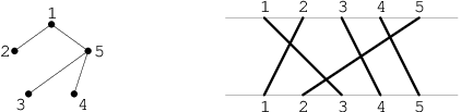
Recognition of PERM. Their recognition is using comparability graphs, based on the following characterization, by Even, Pnueli and Lempel [5]:
To recognize a permutation graph, it is sufficient to check whether both this graph and its complement are comparability graphs. First, by constructing a segment representation, we show that every graph from is also a permutation graph.
Let be a graph from . We can transitively orient its edges and the edges of its complement . Together, the orientations and form a transitive orientation of a complete graph—a linear ordering. See Figure 8.

Now, we have two parallel lines in the plane between which we want to place segments representing the vertices of the graph. On the top line, we place points representing the vertices in the linear ordering given by . For the bottom line, we reverse the orientation and place points according to the linear ordering . To a vertex , we assign the segment .
We need to verify that these segments give an intersection representation of the graph. If two vertices are adjacent, their orders on the top line and on the bottom are different and the corresponding segments intersect. On the other hand, if two vertices are non-adjacent, their orders are the same and the segments do not intersect. So, we obtain a valid intersection representation of the graph which implies is a permutation graph.
To obtain the other inclusion, notice that a segment representation gives transitive orientations and . Another way is to observe that (by reversing the bottom line) and (similarly to function graphs described below).
Extending PERM. A partial representation places several segments between two parallel lines. The problem asks whether it is possible to add the rest of the segments to obtain a representation of a given permutation graph. Notice that all the segments have distinct endpoints.
Let be an input graph. This graph is a permutation graph if and only if and are comparability graphs. The partial representation fixes directions of several edges of and . We orient edges according to the ordering of the endpoints on the top line from left to right. If two segments intersect, the corresponding edge is oriented in , otherwise in .
For the partially oriented and , we run the algorithm for comparability graph extension which is described above. If extending is not possible, the algorithm fails. Otherwise, we obtain transitive orderings and . We place the rest of the points and in the correct order (i.e., on the top line and on the bottom one), and construct a representation of as described above—a vertex is represented by a segment .
Proposition 3
The described algorithm solves correctly, and the running time is .
Proof
If has a segment representation extending the partial representation, then this representation does not change the order of the placed segments. Therefore, the corresponding transitive orientations and have the edges oriented according to the partial representation. It is possible to extend the partially oriented and . Using these orientations, we construct a representation.
The running time is since we need to run two instances of the algorithm solving . To find all the representations, we use that the algorithm for has the same property.
Appendix 0.B Proofs of Lemmas 1, 2, 3, and 5
For a poset and a set , a function is -compatible if we have for any with .
Lemma 6
For every set and every -compatible function there is a -compatible function with .
Proof
The proof goes by induction on . For the conclusion holds trivially. Now, assume . Choose any . Define
where we adopt the convention that and . If and , then there are with , , and , which by -compatibility of implies . Choose any . Set , , and for every . Clearly, the function is -compatible. Therefore, by the induction hypothesis, there is a -compatible function with . It follows that , which completes the proof.∎
Proof (Lemma 1)
Suppose that has a representation extending . Choose any two incomparable vertices and of . The functions and must intersect at some point, which belongs to both and . Hence .
Now, suppose that we have for any two incomparable vertices and of . For convenience, we assume that the coordinates used to describe functions are common for all (we can achieve this by adding new coordinates to the descriptions where necessary). We show how to construct a representation of extending .
First, we define the functions on the coordinates . Let . Define a function by setting for every . Clearly, is -compatible. By Lemma 6, there is a -compatible function with . Set for every .
Now, for any two incomparable vertices and of , we define the functions on an additional coordinate different from and from the coordinates chosen for the other pairs , to ensure that and intersect. The set is non-empty. If has an isolated point , then we have and . Otherwise, is an infinite subset of . Choose and so that and is different from and every other already chosen for a different pair . Let . Define a function by setting and for every . It follows from the definition of and that is -compatible. By Lemma 6, there is a -compatible function with . Set for every . This ensures that and intersect at .
We have defined the functions on a finite set of coordinates . Now, we extend them to the entire so that each of them is linear between any two consecutive coordinates from . It is clear from the construction that for every . Since all functions used for defining on the coordinates from are -compatible, implies . Finally, we have guaranteed that and intersect for any two incomparable vertices and of . Thus is a representation of extending .∎
Proof (Lemma 2)
It suffices that we consider only single steps of reductions 1–3. Clearly, if has a representation extending , then has a representation extending , as all reductions only remove vertices from . To prove the converse implication, suppose that has a representation extending . By Lemma 1, this implies that has a transitive orientation that respects and satisfies for every two incomparable vertices and . We show that has a transitive orientation with the same property, which again by Lemma 1 yields the conclusion.
Suppose that is obtained from by a single step of reduction 1. Let and be the module and the vertex chosen for the reduction step. Choose a transitive orientation of that induces on and arbitrarily orients the internal nodes removed from the modular decomposition by the reduction. By Theorem 4.1, for every we have
and therefore . This implies that is satisfied for any two non-adjacent .
Now, suppose that is obtained from by a single step of reduction 2. Let and be the modules chosen for the reduction step. Choose a transitive orientation of that induces on , orients so that for every represented child and every non-represented child of in the modular decomposition of , and arbitrarily orients the internal nodes removed from the modular decomposition by the reduction. Again, by Theorem 4.1, for every we have
which yields the same conclusion as for reduction 1.
Finally, suppose that is obtained from by a single step of reduction 3. Let the module chosen for the reduction step. Let and be any two represented children of in the modular decomposition of that are consecutive in the order on the represented children of . Choose a transitive orientation of that induces on , orients so that for every non-represented child of in the modular decomposition of , and arbitrarily orients the internal nodes removed from the modular decomposition by the reduction. Let , , and . By Theorem 4.1, we have
This implies that is the region contained between and . In particular, for every other we have . For every that is incomparable to in we have and . Thus we also have .∎
Proof (Lemma 3)
Let be a non-singleton strong module of . If is parallel, then it has just one transitive orientation at all. If is serial and has no non-represented child, then it has only one transitive orientation respecting , as determines the order of representants of the children of . If is serial and has one represented child and one non-represented child, then it has just two transitive orientations, one being the reverse of the other, both respecting . Finally, if is prime, then by Theorem 4.4 it has exactly two transitive orientations, one being the reverse of the other. In the latter case, if has two adjacent represented children, then determines the order of their representants, which shows that only one of the two transitive orientations of respects . Otherwise, both transitive orientations of respect .∎
Appendix 0.C Detailed proof of Theorem 1.2
Below, we describe the construction of the graph in the reduction from 3-SAT in Section 6. For simplicity, we assume that and the literals within each clause are distinct.
The vertex set of consists of a set of vertices corresponding to variables, a set of vertices corresponding to clauses, and two special vertices and , see Fig. 3. Each set corresponding to the variable contains six vertices partitioned into two groups:
Each set corresponding to the clause contains thirteen vertices partitioned into four groups:
The edge set of is defined so that
- •
the vertices from are adjacent to the vertices from ,
- •
the vertices from are adjacent to the vertices from for ,
- •
the vertices from are adjacent to the vertices from ,
- •
is adjacent to the entire ,
- •
is adjacent to the entire ,
- •
is adjacent to ,
- •
there are no other adjacencies.
The modular decomposition of looks as follows:
- •
is a prime module with children , , , and ;
- •
is a parallel module with children ;
- •
each is a serial module with children and ;
- •
each is a parallel module with children , , and ;
- •
each is a parallel module with children , , and ;
- •
is a parallel module with children ;
- •
each is a serial module with children , , , and ;
- •
each is a parallel module with children , , and ;
- •
each is a parallel module with children , , , and .
Now, we construct a partial representation of (see Fig. 4). For a set , let . For , we choose to be intervals of equal length such that
- •
and are singletons, and is entirely to the left of ;
- •
and are singletons, and is entirely to the left of ;
- •
the intervals are pairwise disjoint and contained in .
Next, we define for as follows:
- •
if , then for ;
- •
if , then for ;
- •
, , , and are the closures of the four open intervals that the set splits into;
- •
.
Now, we define all functions for to be constant, as follows:
- •
for ;
- •
;
- •
;
- •
for ;
- •
for .
We can easily check that is indeed a partial representation of .
It remains to prove that is satisfiable if and only if is extendable. To this end, we apply Lemma 5 and prove that is satisfiable if and only if has a transitive orientation that respects and satisfies for any two incomparable vertices and .
We know from Theorem 4.2 that all transitive orientations of are obtained by transitively orienting the strong modules of . All transitive orientations of the strong modules of respecting have the following in common (see Fig. 3):
- •
the module is oriented so that , , and ;
- •
each module is oriented so that .
Thus choosing a transitive orientation of respecting is equivalent to fixing the order of in every and choosing one of the two orientations of every . Figures 5 and 6 illustrate how the regions of the vertices depend on the chosen orientation.
Suppose that is satisfied by a valuation of the variables. This means that in each clause at least one of the literals is true in . We choose transitive orientations of the strong modules of (and thus a transtive orientation of ) so that they respect and satisfy the following:
- •
if is true in , then , otherwise ;
- •
for , where is a literal that is true in .
The region or has non-empty intersection with inside , for and any . The regions and for other choices of and intersect regardless of which transitive orientation we choose.
Now, suppose that is a transitive orientation of with the property that for any two incomparable vertices and . We define a valuation as follows: is true if and only if . Let be the greatest of the modules with respect to . We show that the literal is true in . The regions go below the horizontal line only inside , elsewhere they are blocked from below by functions and for . Thus can intersect or only inside . Suppose . It follows that . If , then the parts of inside are blocked from above by functions and thus lie entirely below the horizontal line , which contradicts the assumption that . Thus we have , which means that the literal is true in . An analogous argument shows that if then is true in . This completes the proof.