Magic Sets for Disjunctive Datalog Programs
Abstract
In this paper, a new technique for the optimization of (partially) bound queries over disjunctive Datalog programs with stratified negation is presented. The technique exploits the propagation of query bindings and extends the Magic Set optimization technique (originally defined for non-disjunctive programs).
An important feature of disjunctive Datalog programs is nonmonotonicity, which calls for nondeterministic implementations, such as backtracking search. A distinguishing characteristic of the new method is that the optimization can be exploited also during the nondeterministic phase. In particular, after some assumptions have been made during the computation, parts of the program may become irrelevant to a query under these assumptions. This allows for dynamic pruning of the search space. In contrast, the effect of the previously defined Magic Set methods for disjunctive Datalog is limited to the deterministic portion of the process. In this way, the potential performance gain by using the proposed method can be exponential, as could be observed empirically.
The correctness of the method is established and proved in a formal way thanks to a strong relationship between Magic Sets and unfounded sets that has not been studied in the literature before. This knowledge allows for extending the method and the correctness proof also to programs with stratified negation in a natural way.
The proposed method has been implemented in the DLV system and various experiments on synthetic as well as on real-world data have been conducted. The experimental results on synthetic data confirm the utility of Magic Sets for disjunctive Datalog, and they highlight the computational gain that may be obtained by the new method with respect to the previously proposed Magic Set method for disjunctive Datalog programs. Further experiments on data taken from a real-life application show the benefits of the Magic Set method within an application scenario that has received considerable attention in recent years, the problem of answering user queries over possibly inconsistent databases originating from integration of autonomous sources of information.
Keywords:
Logic Programming , Stable Models , Magic Sets , Answer Set Programming , Data Integration1 Introduction
Disjunctive Datalog is a language that has been proposed for modeling incomplete data [48]. Together with a light version of negation, in this paper stratified negation, this language can in fact express any query of the complexity class (i.e., ) [22], under the stable model semantics. It turns out that disjunctive Datalog with stratified negation is strictly more expressive (unless the polynomial hierarchy collapses to its first level) than normal logic programming (i.e., non-disjunctive Datalog with unstratified negation), as the latter can express “only” queries in NP. As shown in [22], the high expressive power of disjunctive Datalog has also some positive practical implications in terms of modelling knowledge, since many problems in NP can be represented more simply and naturally in stratified disjunctive Datalog than in normal logic programming. For this reason, it is not surprising that disjunctive Datalog has found several real-world applications [42, 49, 50, 57, 58], also encouraged by the availability of some efficient inference engines, such as DLV [43], GnT [37], Cmodels [46], or ClaspD [21]. As a matter of fact, these systems are continuously enhanced to support novel optimization strategies, enabling them to be effective over increasingly larger application domains. In this paper, we contribute to this development by providing a novel optimization technique, inspired by deductive database optimization techniques, in particular the Magic Set method [6, 9, 63].
The goal of the original Magic Set method (defined for non-disjunctive Datalog programs) is to exploit the presence of constants in a query for restricting the possible search space by considering only a subset of a hypothetical program instantiation that is sufficient to answer the query in question. In order to do this, a top-down computation for answering the query is simulated in an abstract way. This top-down simulation is then encoded by means of rules, defining new Magic Set predicates. The extensions of these predicates (sets of ground atoms) will contain the tuples that are calculated during a top-down computation. These predicates are inserted into the original program rules and can then be used by bottom-up computations to narrow the computation to what is needed for answering the query.
Extending these ideas to disjunctive Datalog faces a major challenge: While non-disjunctive Datalog programs are deterministic, which in terms of the stable model semantics means that any non-disjunctive Datalog program has exactly one stable model, disjunctive Datalog programs are nondeterministic in the sense that they may have multiple stable models. Of course, the main goal is still isolating a subset of a hypothetical program instantiation, upon which the considered query will be evaluated in an equivalent way. There are two basic possibilities how this nondeterminism can be dealt with in the context of Magic Sets: The first is to consider static Magic Sets, in the sense that the definition of the Magic Sets is still deterministic, and therefore the extension of the Magic Set predicates is equal in each stable model. This static behavior is automatic for Magic Sets of non-disjunctive Datalog programs. The second possibility is to allow dynamic Magic Sets, which also introduce non-deterministic definitions of Magic Sets. This means that the extension of the Magic Set predicates may differ in various stable models, and thus can be viewed as being specialized for each stable model.
While the nature of dynamic Magic Sets intuitively seems to be more fitting for disjunctive Datalog than static Magic Sets, considering the architecture of modern reasoning systems for disjunctive Datalog substantiates this intuition: These systems work in two phases, which may be considered as a deterministic (grounding) and a non-deterministic (model search) part. The interface between these two is by means of a ground program, which is produced by the deterministic phase. Static Magic Sets will almost exclusively have an impact on the grounding phase, while dynamic Magic Sets also have the possibility to influence the model search phase. In particular, some assumptions made during the model search may render parts of the program irrelevant to the query, which may be captured by dynamic Magic Sets, but not (or only under very specific circumstances) by static Magic Sets.
In the literature, apart from our own work in [20], there is only one previous attempt for defining a Magic Set method for disjunctive Datalog, reported in [32, 33], which will be referred to as Static Magic Sets () in this work. The basic idea of is that bindings need to be propagated not only from rule heads to rule bodies (as in traditional Magic Sets), but also from one head predicate to other head predicates. In addition to producing definitions for the predicates defining Magic Sets, the method also introduces additional auxiliary predicates called collecting predicates. These collecting predicates however have a peculiar effect: Their use keeps the Magic Sets static. Indeed, both magic and collecting predicates are guaranteed to have deterministic definitions, which implies that disjunctive Datalog systems can exploit the Magic Sets only during the grounding phase. Most systems will actually produce a ground program which does contain neither magic nor collecting predicates.
In this article, we propose a dynamic Magic Set method for disjunctive Datalog with stratified negation under the stable model semantics, provide an implementation of it in the system DLV, and report on an extensive experimental evaluation. In more detail, the contributions are:
-
We present a dynamic Magic Set method for disjunctive Datalog programs with stratified negation, referred to as Dynamic Magic Sets (). Different from the previously proposed static method , existing systems can exploit the information provided by the Magic Sets also during their nondeterministic model search phase. This feature allows for potentially exponential performance gains with respect to the previously proposed static method.
-
We formally establish the correctness of . In particular, we prove that the program obtained by the transformation is query-equivalent to the original program. This result holds for both brave and cautious reasoning.
-
We highlight a strong relationship between Magic Sets and unfounded sets, which characterize stable models. We can show that the atoms which are relevant for answering a query are either true or form an unfounded set, which eventually allows us to prove the query-equivalence results.
-
Our results hold for a disjunctive Datalog language with stratified negation under the stable model semantics. In the literature, several works deal with non-disjunctive Datalog with stratified negation under the well-founded or the perfect model semantics, which are special cases of our language. For the static method , an extension to disjunctive Datalog with stratified negation has previously only been sketched in [33].
-
We have implemented a optimization module inside the DLV system [43]. In this way, we could exploit the internal data-structures of the DLV system and embed in the core of DLV. As a result, the technique is completely transparent to the end user. The system is available at http://www.dlvsystem.com/magic/.
-
We have conducted extensive experiments on synthetic domains that highlight the potential of . We have compared the performance of the DLV system without Magic Set optimization with and with . The results show that in many cases the Magic Set methods yield a significant performance benefit. Moreover, we can show that the dynamic method can yield drastically better performance than the static . Importantly, in cases in which cannot be beneficial (if all or most of the instantiated program is relevant for answering a query), the overhead incurred is very light.
-
We also report on experiments which evaluate the impact of on an industrial application scenario on real-world data. The application involves data integration and builds on several results in the literature (for example [5, 7, 14, 16, 17, 31]), which transform the problem of query answering over inconsistent databases (in this context stemming from integrating autonomous data sources) into query answering over disjunctive Datalog programs. By leveraging these results, can be viewed as a query optimization method for inconsistent databases or for data integration systems. The results show that can yield significant performance gains for queries of this application.
Organization.
The main body of this article is organized as follows. In Section 2, preliminaries on disjunctive Datalog and on the Magic Set method for non-disjunctive Datalog queries are introduced. Subsequently, in Section 3 the extension for the case of disjunctive Datalog programs is presented, and we show its correctness. In Section 4 we discuss the implementation and integration of the Magic Set method within the DLV system. Experimental results on synthetic benchmarks are reported in Section 5, while the application to data integration and its experimental evaluation is discussed in Section 6. Finally, related work is discussed in Section 7, and in Section 8 we draw our conclusions.
2 Preliminaries
In this section, (disjunctive) Datalog programs with (stratified) negation are briefly described, and the standard Magic Set method is presented together with the notion of sideways information passing strategy (SIPS) for Datalog rules.
2.1 Disjunctive Datalog Programs with Stratified Negation
In this paper, we adopt the standard Datalog name convention: Alphanumeric strings starting with a lowercase character are predicate or constant symbols, while alphanumeric strings starting with an uppercase character are variable symbols; moreover, we allow the use of positive integer constant symbols. Each predicate symbol is associated with a non-negative integer, referred to as its arity. An atom is composed of a predicate symbol and a list = of terms, each of which is either a constant or a variable. A literal is an atom or a negated atom ; in the first case the literal is positive, while in the second it is negative.
A disjunctive Datalog rule with negation (short: Datalog∨,¬ rule) is of the form
where are atoms and . The disjunction is the head of , while the conjunction is the body of . Moreover, denotes the set of head atoms, while denotes the set of body literals. We also use and for denoting the sets of atoms appearing in positive and negative body literals, respectively. If is disjunction-free, that is , and negation-free, that is is empty, then we say that is a Datalog rule; if is empty in addition, then we say that is a fact. A disjunctive Datalog program is a finite set of rules; if all the rules in it are disjunction- and negation-free, then is a (standard) Datalog program.
Given a Datalog∨,¬ program , a predicate belongs to the Intensional Database (IDB) if it is either in the head of a rule with non-empty body, or in the head of a disjunctive rule; otherwise, it belongs to the Extensional Database (EDB). The set of rules having IDB predicates in their heads is denoted by , while denotes the remaining rules, that is, . For simplicity, we assume that predicates will always be of the same type (EDB or IDB) in any program.
The set of all constants appearing in a program is the universe of and is denoted by ,11 1 If has no constants, an arbitrary constant is added to . while the set of ground atoms constructable from predicates in with constants in is the base of , denoted by . We call an atom (rule, or program) ground if it does not contain any variables. A substitution is a function from variables to elements of . For an expression (atom, literal, rule), by we denote the expression obtained from by substituting all occurrences of each variable in with . A ground atom (resp. ground rule ) is an instance of an atom (resp. rule ) if there is a substitution from the variables in (resp. in ) to such that (resp. ). Given a program , denotes the set of all possible instances of rules in .
Given an atom and a set of ground atoms , by we denote the set of ground instances of belonging to . For example, is the set of all ground atoms obtained by applying to all the possible substitutions from the variables in to , that is, the set of all the instances of . Abusing notation, if is a set of atoms, by we denote the union of all , for each .
A desirable property of Datalog∨,¬ programs is safety. A Datalog∨,¬ rule is safe if each variable appearing in appears in at least one atom of . A Datalog∨,¬ program is safe if all its rules are safe. Moreover, programs without recursion over negated literals constitute an interesting class of Datalog∨,¬ programs. Without going into details, a predicate in the head of a rule depends on all the predicates in the body of ; depends on positively if appears in , and depends on negatively if appears in . A program has recursion over negation if a cycle of dependencies with at least one negative dependency exists. If a program has no recursion over negation, then the program is stratified (short: Datalog). In this work only safe programs without recursion over negation are considered.
An interpretation for a program is a subset of . A positive ground literal is true with respect to an interpretation if ; otherwise, it is false. A negative ground literal is true with respect to if and only if is false with respect to , that is, if and only if . The body of a ground rule is true with respect to if and only if all the body literals of are true with respect to , that is, if and only if and . An interpretation satisfies a ground rule if at least one atom in is true with respect to whenever the body of is true with respect to . An interpretation is a model of a Datalog∨,¬ program if satisfies all the rules in . Since an interpretation is a set of atoms, if is an interpretation for a program , and is another program, then by we denote the restriction of to the base of .
Given an interpretation for a program , the reduct of with respect to , denoted by , is obtained by deleting from all the rules with , and then by removing all the negative literals from the remaining rules.
The semantics of a Datalog∨,¬ program is given by the set of stable models of , where an interpretation is a stable model for if and only if is a subset-minimal model of . It is well-known that there is exactly one stable model for any Datalog program, also in presence of stratified negation. However, for a Datalog program , holds (Datalog∨,¬ programs, instead, can also have no stable model).
Given a ground atom and a Datalog∨,¬ program , is a cautious (or certain) consequence of , denoted by , if for each ; is a brave (or possible) consequence of , denoted by , if for some . Note that brave and cautious consequences coincide for Datalog programs, as these programs have a unique stable model. Moreover, cautious consequences of a Datalog program are also brave consequences of because holds in this case.
Given a query (an atom),22 2 Note that more complex queries can still be expressed using appropriate rules. We assume that each constant appearing in also appears in ; if this is not the case, then we can add to a fact such that is a predicate not occurring in and are the arguments of . Question marks will be usually omitted when referring to queries in the text. denotes the set of all substitutions for the variables of such that , while denotes the set of substitutions for the variables of such that .
Let and be two Datalog∨,¬ programs and a query. Then and are brave-equivalent with respect to , denoted by , if is guaranteed for each set of facts defined over predicates which are EDB predicates of or ; similarly, and are cautious-equivalent with respect to , denoted by , if is guaranteed for each set of facts defined over predicates which are EDB predicates of or .
2.2 Bottom-up Disjunctive Datalog Computation
Many Datalog∨,¬ systems implement a two-phase computation. The first phase, referred to as program instantiation or grounding, is bottom-up. For an input program , it produces a ground program which is equivalent to , but significantly smaller. Most of the techniques used in this phase stem from bottom-up methods developed for classic and deductive databases; see for example [1] or [28, 43] for details. Essentially, predicate instances which are known to be true or known to be false are identified and this knowledge is used for deriving further instances of this kind. Eventually, the truth values obtained in this way are used to produce rule instances which are not satisfied already. It is important to note that this phase behaves in a deterministic way with respect to stable models. No assumptions about truth or falsity of atoms are made, only definite knowledge is derived, which must hold in all stable models. For this reason, programs with multiple stable models cannot be solved by grounding.
The second phase is often referred to as stable model search and takes care of the non-deterministic computation. Essentially, one undefined atom is selected and its truth or falsity is assumed. The assumption might imply truth or falsity of other undefined atoms. Hence, the process is repeated until either an inconsistency is derived or all atoms have been interpreted. In the latter case an additional check is performed to ensure stability of the model. Details on this process can be found for example in [23]. Query answering is typically handled by storing all admissible answer substitutions as stable models are computed. For brave reasoning, each stable model can contribute substitutions to the set of answers. In this case the set of answers is initially empty. For cautious reasoning, instead, each stable model may eliminate some substitutions from the set of admissible answers. Therefore, in this case all possible substitutions for the input query are initially contained in the set of answers.
2.3 Sideways Information Passing for Datalog Rules
The Magic Set method aims at simulate a top-down evaluation of a query , like for instance the one adopted by Prolog. According to this kind of evaluation, all the rules such that and (for some substitution for all the variables of and some substitution for all the variables of ) are considered in a first step. Then the atoms in are taken as subqueries (we recall that standard Datalog rules have empty negative body), and the procedure is iterated. Note that, according to this process, if a (sub)query has some argument that is bound to a constant value, this information is “passed” to the atoms in the body. Moreover, the body is considered to be processed in a certain sequence, and processing a body atom may bind some of its arguments for subsequently considered body atoms, thus “generating” and “passing” bindings within the body. Whenever a body atom is processed, each of its argument is therefore considered to be either bound or free. We illustrate this mechanism by means of an example.
Example 2.1
Let be a query for a program having the following inference rules:
Since this is a Datalog program, brave and cautious consequences coincide. Moreover, let be the EDB of the program. A top-down evaluation scheme considers and with and bound to and , respectively. In particular, when considering , the information about the binding of the two variables is passed to , which is indeed the only query atom occurring in . Thus, the evaluation fails since does not occur in .
When considering , instead, the binding information can be passed either to or to . Suppose that atoms are evaluated according to their ordering in the rule (from left to right); then is considered before . In particular, contains the atom , which leads us to map to . Eventually, this inferred binding information might be propagated to the remaining body atom , which hence becomes .
The process has now to be repeated by looking for an answer to . Again, rule can be considered, from which we conclude that this query is true since occurs in . Thus, holds as well due to .
Note that in the example above we have two degrees of freedom in the specification of the top-down evaluation scheme. The first one concerns which ordering is used for processing the body atoms. While Prolog systems are usually required to follow the ordering in which the program is written, Datalog has a purely declarative semantics which is independent of the body ordering, allowing for an arbitrary ordering to be adopted. The second degree of freedom is slightly more subtle, and concerns the selection of the terms to be considered bound to constants from previous evaluations. Indeed, while we have considered the propagation of all the binding information that originates from previously processed body atoms, it is in general possible to restrict the top-down evaluation to partially propagate this information. For instance, one may desire to propagate only information generated from the evaluation of EDB predicates, or even just the information that is passed on via the head atom.
The specific propagation strategy adopted in the top-down evaluation scheme is called sideways information passing strategy (SIPS), which is just a way of formalizing a partial ordering over the atoms of each rule together with the specification of how the bindings originated and propagate [9, 33]. To formalize this concept, in what follows, for each IDB atom , we shall denote its associated binding information (originated in a certain step of the top-down evaluation) by means of a string built over the letters and , denoting “bound” and “free”, respectively, for each argument of .
Definition 2.2 (SIPS for Datalog rules)
A SIPS for a Datalog rule with respect to a binding for the atom is a pair , where:
- 1.
is a strict partial order over the atoms in , such that , for all atoms ; and,
- 2.
is a function assigning to each atom a subset of the variables in —intuitively, those made bound when processing .
Intuitively, for each atom occurring in , the strict partial order specifies those atoms that have to be processed before processing atom . Eventually, an argument of is bound to a constant if there exists an atom such that and . Note that the head atom precedes all other atoms in .
Example 2.3
The SIPS we have adopted in Example 2.1 for with respect to the binding (originating from the query ) can be formalized as the pair , where , , and . Instead, the SIPS we have adopted for with respect to the binding can be formalized as the pair , where , and .
All the algorithms and techniques we shall develop in this paper are orthogonal with respect to the underlying SIPSes to be used in the top-down evaluation. Thus, in Section 2.4, we shall assume that Datalog programs are provided in input together with some arbitrarily defined SIPS , for each rule and for each possible adornment for the head atom in .
2.4 Magic Sets for Datalog Programs
The Magic Set method is a strategy for simulating the top-down evaluation of a query by modifying the original program by means of additional rules, which narrow the computation to what is relevant for answering the query. We next provide a brief and informal description of the Magic Set rewriting technique. The reader is referred to [63] for a detailed presentation.
The method is structured in four main phases, which are informally illustrated below by means of Example 2.1.
(1) Adornment. The key idea is to materialize the binding information for IDB predicates that would be propagated during a top-down computation. In particular, the fact that an IDB predicate is associated with a binding information (i.e., a string over the letters and , one for each term in ) is denoted by the atom obtained adorning the predicate symbol with the binding at hand, that is, by . In what follows, the predicate is said to be an adorned predicate.
First, adornments are created for query predicates so that an argument occurring in the query is adorned with the letter if it is a constant, or with the letter if it is a variable. For instance, the adorned version of the query atom is , which gives rise to the adorned predicate .
Each adorned predicate is eventually used to propagate its information into the body of the rules defining it according to a SIPS, thereby simulating a top-down evaluation. In particular, assume that the binding has to be propagated into a rule whose head is . Thus, the associated SIPS determines which variables will be bound in the evaluation of the various body atoms. Indeed, a variable of an atom in is bound if and only if either
- 1.
with ; or,
- 2.
for an atom such that holds.
Adorning a rule with respect to an adorned predicate means propagating the binding information , starting from the head predicate , thereby creating a novel adorned rule where all the IDB predicates in are substituted by the adorned predicates originating from the binding according to (1) and (2).
Example 2.4
Adorning the query generates . Then, propagating the binding information into the rule , i.e., when adorning with , produces the following adorned rule (recall here that adornments apply only to IDB predicates, whereas is an EDB predicate):
Instead, when propagating into the rule according to the SIPS defined in Example 2.3, we obtain the following adorned rule:
While adorning rules, novel binding information in the form of yet unseen adorned predicates may be generated, which should be used for adorning other rules. In fact, the adornment step is repeated until all bindings have been processed, yielding the adorned program, which is the set of all adorned rules created during the computation. For instance, in the above example, the adorned program just consists of and for no adorned predicate different from is generated.
(2) Generation. In the second step of the Magic Set method, the adorned program is used to generate magic rules, which are used to simulate the top-down evaluation scheme and to single out the atoms relevant for answer the input query. For an adorned atom , let be its magic version defined as the atom , where is obtained from by eliminating all arguments corresponding to an label in , and where is a new predicate symbol (for simplicity denoted by attaching the prefix “” to the predicate symbol ). Intuitively, ( a substitution) is inferred by the rules of the rewritten program whenever a top-down evaluation of the original program would process a subquery of the form , where is obtained from by applying to all terms in .
Thus, if is an adorned atom (i.e., is not the empty string) in the body of an adorned rule having in head, a magic rule is generated such that (i) and (ii) is the union of and the set of all the atoms such that .
Example 2.5
In our running example, only one magic rule is generated,
In fact, the adorned rule does not produce any magic rule, since there is no adorned predicate in .
(3) Modification. The adorned rules are subsequently modified by adding magic atoms to their bodies. These magic atoms limit the range of the head variables avoiding the inference of facts which cannot contribute to the derivation of the query. In particular, each adorned rule , whose head atom is , is modified by adding the atom to its body. The resulting rules are called modified rules.
Example 2.6
In our running example, the following modified rules are generated:
(4) Processing the Query. Finally, given the adorned predicate obtained when adorning a query , (1) a magic seed (a fact) and (2) a rule are produced. In our example, and are generated.
The complete rewritten program according to the Magic Set method consists of the magic, modified, and query rules (together with the original EDB). Given a Datalog program , a query , and the rewritten program , it is well-known that and are equivalent with respect to , i.e., and hold [63].
Example 2.7
The complete rewriting of our running example is as follows:33 3 The Magic Set rewriting of a program affects only , so we usually omit in examples.
In this rewriting, represents a potential sub-path of the paths from to . Therefore, when answering the query, only these sub-paths will be actually considered in the bottom-up computation. One can check that this rewriting is in fact equivalent to the original program with respect to the query .
3 Magic Set Method for Datalog Programs
In this section we present the Dynamic Magic Set algorithm () for the optimization of disjunctive programs with stratified negation. Before discussing the details of the algorithm, we informally present the main ideas that have been exploited for enabling the Magic Set method to work on disjunctive programs (without negation).
3.1 Overview of Binding Propagation in Datalog∨ Programs
As first observed in [33], while in non-disjunctive programs bindings are propagated only head-to-body, a Magic Set transformation for disjunctive programs has to propagate bindings also head-to-head in order to preserve soundness. Roughly, suppose that a predicate is relevant for the query, and a disjunctive rule contains in the head. Then, besides propagating the binding from to the body of (as in the non-disjunctive case), the binding must also be propagated from to the other head atoms of . The reason is that any atom which is true in a stable model needs a supporting rule, which is a rule with a true body and in which the atom in question is the only true head atom. Therefore, can yield support to the truth of only if all other head atoms are false, which is due to the implicit minimality criterion in the semantics.
Consider, for instance, a Datalog∨ program consisting of the rule , and the query . Even though the query propagates the binding for the predicate , in order to correctly answer the query we also need to evaluate the truth value of , which indirectly receives the binding through the body predicate . For instance, suppose that the program contains the facts and ; then the atom is relevant for the query (i.e., it should belong to the Magic Set of the query), since the truth of would invalidate the derivation of from the above rule, due to the minimality of the semantics. It follows that, while propagating the binding, the head atoms of disjunctive rules must be all adorned as well.
However, the adornment of the head of one disjunctive rule may give rise to multiple rules, having different adornments for the head predicates. This process can be somehow seen as “splitting” into multiple rules. While this is not a problem in the non-disjunctive case, the semantics of a disjunctive program may be affected. Consider, for instance, the program consisting of the rule , in which and are mutually exclusive (due to minimality) since they do not appear in any other rule head. Assuming the adornments and to be propagated, we might obtain rules whose heads have the form (derived while propagating ) and (derived while propagating ). These rules could support two atoms and , while in the original program and could not hold simultaneously (due to semantic minimality), thus changing the original semantics.
The method proposed in [33] circumvents this problem by using some auxiliary predicates that collect all facts coming from the different adornments. For instance, in the above example, two rules of the form and are added for the predicate . The main deficiency of this approach is that collecting predicates will store a sizable superset of all the atoms relevant to answer the given query.
An important observation is that these collecting predicates are defined in a deterministic way. Since these predicates are used for restricting the computation in [33], a consequence is that assumptions during the computation cannot be exploited for determining the relevant part of the program. In terms of bottom-up systems, this implies that the optimization affects only the grounding portion of the solver. Intuitively, it would be beneficial to also have a form of conditional relevance, exploiting also relevance for assumptions. In fact, in Section 5, we provide experimental evidence for this intuition.
In the following, we propose a novel Magic Set method that guarantees query equivalence and also allows for the exploitation of conditional or dynamic relevance, overcoming a major drawback of .
3.2 Algorithm
Our proposal to enhance the Magic Set method for disjunctive Datalog programs has two crucial features compared to the one of [33]:
- 1.
First, the semantics of the program is preserved by stripping off the adornments from non-magic predicates in modified rules, and not by introducing collecting predicates that can introduce overhead in the grounding process, as discussed in Section 3.1.
- 2.
Second, the proposed Magic Set technique is not just a way to cut irrelevant rules from the ground program; in fact, it allows for dynamic determination of relevance, thus optimizing also the nondeterministic computation by disabling parts of the programs which are not relevant in any extension of the current computation state.
Algorithm DMS(,) Input: A Datalog program , and a query Output: The rewritten program ; var: , : set of adorned predicates; Q,P,Q,P: set of rules; begin 1. := ; := ; Q,P := ; Q,P := {BuildQuerySeed()}; 2. while do 3. := an element of ; remove from ; add to ; 4. for each rule and for each atom do 5. :=Adorn; 6. Q,P := Q,P Generate; 7. Q,P := Q,P Modify ; 8. end for 9. end while 10. :=Q,P Q,P ; 11. return ; end.
The algorithm implementing these strategies is reported in Figure 1 as pseudo-code. We assume that all variables are passed to functions by reference, in particular the variable is modified inside BuildQuerySeed and Adorn. Its input is a Datalog program44 4 Note that the algorithm can be used for non-disjunctive and/or positive programs as a special case. and a query . The algorithm uses two sets, and , to store adorned predicates to be propagated and already processed, respectively. After all the adorned predicates have been processed, the method outputs a rewritten program consisting of a set of modified and magic rules, stored by means of the sets Q,P and Q,P, respectively (together with the original EDB). The main steps of the algorithm are illustrated by means of the following running example.
Example 3.1 (Strategic Companies [15])
Let be a collection of companies producing some goods in a set , such that each company is controlled by a set of other companies . A subset of the companies is a strategic set if it is a minimal set of companies satisfying the following conditions: Companies in produce all the goods in ; and implies , for each .
We assume that each product is produced by at most two companies and that each company is controlled by at most three companies. It is known that the problem retains its hardness (for the second level of the polynomial hierarchy; see [15]) under these restrictions. We assume that production of goods is represented by an EDB containing a fact for each product produced by companies and , and that the control is represented by facts for each company controlled by companies , , and .55 5 If a product is produced by only one company, , and similarly for companies controlled by fewer than three companies. This problem can be modeled via the following disjunctive program :
Moreover, given a company , we consider a query asking whether belongs to some strategic set of .
Function BuildQuerySeed(, ) Input: : query; : set of adorned predicates; Output: The query seed (a magic atom); var: : adornment string; begin 1. Let be the atom in . 2. ; 3. for each argument in do 4. if is a constant then ; else ; end if 5. end for 6. add to ; 7. return ; end.
The computation starts in step 1 by initializing , , and Q,P to the empty set. Then, the function BuildQuerySeed is used for storing in Q,P the magic seed, and inserting in the set the adorned predicate of . Note that we do not generate any query rules because standard atoms in the transformed program will not contain adornments. Details of BuildQuerySeed are reported in Figure 2.
Example 3.2
Given the query and the program , function BuildQuerySeed creates the fact and inserts in .
Function Adorn(, , , ) Input: : rule; : adorned atom; , : set of adorned predicates; Output: an adorned rule; var: : adorned rule; : adornment string; begin 1. Let be the SIPS associated with and . 2. ; 3. for each IDB atom in do 4. ; 5. for each argument in do 6. if is a constant then 7. ; 8. else 9. Argument is a variable. Let be this variable. 10. if or there is in such that 11. and then 12. ; 13. else 14. ; 15. end if 16. end if 17. end for 18. substitute in with ; 19. if set does not contain then add to ; end if 20. end for 21. return ; end.
The core of the algorithm (steps 3–8) is repeated until the set is empty, i.e., until there is no further adorned predicate to be propagated. In particular, an adorned predicate is moved from to in step 3, and its binding is propagated in each (disjunctive) rule of the form
(with ) having an atom in the head (note that the rule is processed a number of times that equals the number of head atoms with predicate ; steps 4–8).
(1) Adornment. Step 5 in Figure 1 implements the adornment of the rule. Different from the case of non-disjunctive positive programs, the binding of the predicate needs to be also propagated to the atoms in the head. Therefore, binding propagation has to be extended to the head atoms different from , which are therefore adorned according to a SIPS specifically conceived for disjunctive programs. Notation gets slightly more involved here: Since in non-disjunctive rules there is a single head atom, it was sufficient to specify an order and a function for each of its adornments (omitting the head atom in the notation). With disjunctive rules, an order and a function need to be specified for each adorned head atom, so it is no longer sufficient to include only the adornment in the notation, but we rather include the full adorned atom.
Definition 3.3 (SIPS for Datalog rules)
A SIPS for a Datalog rule with respect to a binding for an atom is a pair , where:
- 1.
is a strict partial order over the atoms in , such that:
- (a)
, for all atoms different from ;
- (b)
for each pair of atoms and , does not hold; and,
- (a)
- 2.
is a function assigning to each atom a subset of the variables in —intuitively, those made bound when processing .
As for Datalog rules, for each atom occurring in , the strict partial order specifies those atoms that have to be processed before processing atom , and an argument of is bound to a constant if there exists an atom occurring in such that and . The difference with respect to SIPSes for Datalog rules is precisely in the dependency from in addition to , and in condition (1.b) stating that head atoms different from and negative body literals cannot provide bindings to variables of other atoms.
The underlying idea is that a rule which is used to “prove” the truth of an atom in a top-down method will be a rule which supports that atom. This implies that all other head atoms in that rule must be false and that the body must be true. Head atoms and atoms occurring in the negative body cannot “create” bindings (that is, restrict the values of variables), but these atoms are still relevant to the query, which leads to the restrictions in Definition 3.3.
Note that this definition considers each rule in isolation and is therefore independent of the inter-rule structure of a program. In particular, it is not important for the SIPS definition whether a program is cyclic or contains head cycles.
In the following, we shall assume that each Datalog program is provided in input together with some arbitrarily defined SIPS for Datalog rules . In fact, armed with , the adornment can be carried out precisely as we discussed for Datalog programs; in particular, we recall here that a variable of an atom in is bound if and only if either:
- 1.
with ; or,
- 2.
for an atom such that holds.
The function Adorn produces an adorned disjunctive rule from an adorned atom and a suitable unadorned rule (according to the bindings defined in the points (1) and (2) above), by inserting all newly adorned predicates in . Hence, in step 5 the rule is of the form
Details of Adorn are reported in Figure 3.
Example 3.4
Let us resume from Example 3.2. We are supposing that the adopted SIPS is passing the bindings via and to the variables of atoms, in particular
When is removed from the set , we first select rule and the head predicate . Then the adorned version is
Next, is processed again, this time with head predicate , producing
Finally, processing we obtain
Function Generate(, , ) Input: : rule; : adorned atom; : adorned rule; Output: a set of magic rules; var: : set of rules; : rule; begin 1. Let be the SIPS associated with and . 2. ; 3. for each atom in different from do 4. if then 5. ; 6. for each atom in such that do 7. add atom to ; 8. end for 9. ; 10. end if 11. end for 12. return ; end.
(2) Generation. The algorithm uses the adorned rule for generating and collecting the magic rules in step 6 (Figure 1). More specifically, Generate produces magic rules according to the following schema: if is an adorned atom (i.e., is not the empty string) occurring in and different from , a magic rule is generated such that (i) and (ii) is the union of and the set of all the atoms such that . Details of Generate are reported in Figure 4.
Example 3.5
Continuing with our running example, by invoking Generate, the following magic rule is produced:
Similarly, by invoking Generate, the following magic rule is produced:
Finally, the following magic rules are produced by Generate:
(3) Modification. In step 7 the modified rules are generated and collected. The only difference with respect to the Datalog case is that the adornments are stripped off the original atoms. Specifically, given an adorned rule associated with a rule , a modified rule is obtained from by adding to its body an atom for each atom occurring in . Hence, the function Modify, reported in Figure 5, constructs a rule of the form
Function Modify(, ) Input: : rule; : adorned rule; Output: a modified rule; var: : rule; begin 1. ; 2. for each atom in do 3. add to ; 4. end for 5. return ; end.
Finally, after all the adorned predicates have been processed, the algorithm outputs the program .
Example 3.6
In our running example, we derive the following set of modified rules:
Here, (resp. , ) is derived by adding magic predicates and stripping off adornments for the rule (resp. , ). Thus, the optimized program comprises the above modified rules as well as the magic rules in Example 3.5, and the magic seed (together with the original EDB).
Before establishing the correctness of the technique, we briefly present an example of the application of on a program containing disjunction and stratified negation.
Example 3.7
Let us consider a slight variant of the Strategic Companies problem described in Example 3.1 in which we have to determine whether a given company does not belong to any strategic set. We can thus consider the query for the program obtained by adding to the following rule:
where is an EDB predicate. Company does not belong to any strategic set if the query is cautiously false.
In this case, processing the query produces the query seed (a fact) and the adorned predicate (which is added to set ). After that, is moved from to and rule is considered. Assuming the following SIP:
by invoking Adorn we obtain the following adorned rule:
The new adorned predicate is added to . Then, Generate and Modify produce the following magic and modified rules:
The algorithm then processes the adorned atom . Hence, if the SIPS presented in Example 3.4 is assumed, the rewritten program comprises the following rules: , , , , , , , , and .
3.3 Query Equivalence Result
We conclude the presentation of the algorithm by formally proving its correctness. We would like to point out that all of these results hold for any kind of SIPS, as long as it conforms to Definition 3.3. Therefore, in the remainder of this section, we assume that any program comes with some associated SIPS. In the proofs, we use the well established notion of unfounded set for disjunctive Datalog programs (possibly with negation) defined in [44]. Before introducing unfounded sets, however, we have to define partial interpretations, that is, interpretations for which some atoms may be undefined.
Definition 3.8 (Partial Interpretation)
Let be a Datalog∨,¬ program. A partial interpretation for is a pair such that . The atoms in are interpreted as true, while the atoms in are not false and those in are undefined. All other atoms are false.
Note that total interpretations are a special case in which . We can then formalize the notion of unfounded set.
Definition 3.9 (Unfounded Sets)
Let be a partial interpretation for a Datalog∨,¬ program , and be a set of atoms. Then, is an unfounded set for with respect to if and only if, for each ground rule with , at least one of the following conditions holds: ; ; ; .
Intuitively, conditions , and check if the rule is satisfied by regardless of the atoms in , while condition checks whether the rule can be satisfied by taking the atoms in as false.
Example 3.10
Consider again the program of Example 3.1 and assume . Then consists of the rule
(together with facts, and rules having some ground instance of EDB predicate not occurring in , omitted for simplicity). Consider now a partial interpretation such that . Thus, is an unfounded set for with respect to ( satisfies condition of Definition 3.9), while is not ( violates all conditions).
The following is an adaptation of Theorem 4.6 in [44] to our notation.
Theorem 3.11 ([44])
Let be a partial interpretation for a Datalog∨,¬ program . Then, for any stable model of such that , and for each unfounded set of with respect to , holds.
Example 3.12
In Example 3.10, we have shown that is an unfounded set for with respect to . Note that the total interpretation is a stable model of , and that the unfounded set is disjoint from .
Equipped with these notions and Theorem 3.11, we now proceed to prove the correctness of the strategy. In particular, we shall first show that the method is sound in that, for each stable model of , there is a stable model of such that (i.e., the two models coincide when restricted to the query). Then, we prove that the method is also complete, i.e., for each stable model of , there is a stable model of such that .
In both parts of the proof, we shall exploit the following (syntactic) relationship between the original program and the transformed one.
Lemma 3.13
Let be a Datalog program, a query, and let be a ground atom66 6 Note that in this way the lemma refers only to rules that contain a head atom for which a magic predicate has been generated during the transformation. in (the base of the transformed program). Then the ground rule
belongs to if and only if the ground rule
belongs to .
Proof. Consider the following rule such that for some substitution :
Since is a ground atom in , has been inserted in the set at some point of the Magic Set transformation, and it has eventually been used to adorn and modify , thereby producing the following rule :
Clearly enough, the substitution mapping into can also be used to map into , since the magic atoms added into the positive body of are defined over a subset of the variables occurring in head atoms.
Let be a rule such that for some substitution :
By the construction of , is a modified rule produced by adding some magic atom to the positive body of a rule of the form:
Thus, the substitution mapping to can also be used to map to , since and have the same variables.
3.3.1 Soundness of the Magic Set Method
Let us now start with the first part of the proof, in particular, by stating some further definitions and notations. Given a model of , and a model of , we next define the set of atoms which are relevant for but are false with respect to .
Definition 3.14 (Killed Atoms)
Given a model for , and a model of , the set of the killed atoms with respect to and is defined as:
Example 3.15
We consider the program presented in Section 3.2 (we recall that ), the EDB introduced in Example 3.10, and a stable model for . Thus, consists of the following rules:
Since is also a model of the program above, we can compute and check that belongs to it because of in . Note that, by definition, also false ground instances of EDB predicates like or belong to . Moreover, note that no other atom belongs to this set.
The intuition underlying the definition above is that killed atoms are either false ground instances of some EDB predicate, or false atoms which are relevant with respect to (for there exists an associated magic atom in the model ); since is a model of contained in , we expect that these atoms are also false in any stable model for containing (which, we recall here, is the model restricted on the atoms originally occurring in ).
Example 3.16
Let us resume from Example 3.15. We have that , which coincides with model of Example 3.10. Hence, we already know that is an unfounded set for with respect to . Since each other atom in is such that is an EDB predicate, we also have that is an unfounded set for with respect to . Therefore, as a consequence of Theorem 3.11, each stable model of such that (in this case only itself) is disjoint from .
This intuition is formalized below.
Proposition 3.17
Let be a model for , and be a model of . Then, is an unfounded set for with respect to .
Proof. According to Definition 3.9 of unfounded sets (for with respect to ), given any rule in of the form
we have to show that if , then at least one of the following conditions holds: ; ; ; .
Note that the properties above refer to the original program . However, our hypothesis is formulated over the transformed one (for instance, we know that is a model of ). The line of the proof is then to analyze in the light of its syntactic relationships with established via Lemma 3.13. In particular, recall first that, by Definition 3.14, there is a binding such that (and, hence, is a ground atom in ). Thus, we can apply Lemma 3.13 and conclude the existence of a ground rule such that:
Since is a model of , the proof is just based on analyzing the following three scenarios that exhaustively cover all possibilities (concerning the fact that the rule is satisfied by ):
- (S1)
-
, i.e., the negative body of is false with respect to ;
- (S2)
-
, i.e., the positive body of is false with respect to ;
- (S3)
-
, , and , i.e., none of the previous cases holds, and hence the head of is true with respect to .
In the remaining, we shall show that (S1) implies condition , (S2) implies condition (2), and (S3) implies either (2) or (3). In fact, note that condition cannot hold.
- (S1)
-
Assume that . Since and , from we immediately conclude , i.e., holds.
- (S2)
-
Assume that , and let be a modified rule such that for some substitution :
We first claim that must hold in this case. To prove the claim, observe that during the Generation step preceding the production of , a magic rule such that and has been produced for each (we recall that magic rules have empty negative bodies). Hence, since the variables of are a subset of the variables of , by applying the substitution to we obtain a ground rule such that and . Thus, if , from the above magic rules and since is a model containing by assumption, then we would conclude that . However, this is impossible, since and imply .
Now, implies the existence of an atom such that , that is, . In particular, we can assume w.l.o.g. that, for any with , it is the case that , where is the rule in from which the modified rule has been generated (just take a -minimum element in ). If is an EDB predicate, the atom belongs to by the definition of killed atoms. Otherwise, is an IDB predicate. In this case, there is a magic rule , produced during the Generation step preceding the production of , such that and . Thus, belongs to . In particular, holds because belongs to and by the properties of . Therefore, since is a model of , belongs to , from which follows from the definition of killed atoms. Thus, independently of the type (EDB, IDB) of , (2) holds.
- (S3)
-
Assume that , , and . First, observe that from we can conclude that there is a rule in obtained from by removing its negative body literals. Consider now the rules produced during the Generation step, for each (as in (S2)). We distinguish two cases.
If , since , we can conclude that , for each . Moreover, since is a model of , the latter implies that , for each . Then holds, and so (because is a model of ). We now observe that is equivalent to . Moreover, the latter is equivalent to because contains only standard atoms and . In addition, from we conclude , and by Definition 3.14, holds. Hence, , which is not empty, and so condition holds.
Otherwise, . Let be such that and, for any , implies (where is the rule in from which the modified rule has been generated). If is an EDB predicate, the atom belongs to by the definition of killed atoms. Otherwise, is an IDB predicate and there is a magic rule having an atom in head, and such that . Therefore, belongs to , from which follows from the definition of killed atoms. Thus, independently of the type (EDB, IDB) of , (2) holds.
We can now complete the first part of the proof.
Lemma 3.18
For each stable model of , there is a stable model of such that .
Proof. Let be a stable model of , the program obtained by adding to a fact for each atom in . We shall show that is in fact a stable model of such that . Of course, is a model of such that . So, the line of the proof is to show that if is not stable, then it is possible to build a model of such that , thereby contradicting the minimality of over the models of .
Assume, for the sake of contradiction, that is not stable and let be a model of . Define as the interpretation . By construction, note that , since coincides with . In fact, in the case where , we would have that , since and are disjoint. Hence, would not only be a model for but also a model for , while on the other hand holds. However, this is impossible, since is a stable model of . So, must hold. Hence, to complete the proof and get a contradiction, it remains to show that is actually a model of , i.e., it satisfies all the rules in . To this end, we have to consider the following two kinds of rules:
- (1)
-
Consider a ground magic rule such that , and let be the (only) atom in . Since , implies that . In fact, since is a model of and , must hold (we recall that ). Moreover, since does not contain any magic atom, is also contained in . Thus, by the construction of , we can conclude that .
- (2)
-
Consider a rule obtained by removing the negative literals from a ground modified rule where
and where . Observe that holds by the definition of reduct. Moreover, let be the rule of associated with (according to Lemma 3.13):
We have to show that . The proof is based on establishing the following properties on and :
(1) (2) (3) (4) (5) In particular, we shall directly prove (1), and show the following implications: (1)(2)(3), (2)(4), and (3)(5). Eventually, based on (4) and (5), the fact that can be easily derived as follows: Since , by the definition of we can conclude that . Moreover, because of (4) and the fact that , coincides in turn with . Then, recall that . Thus, , which is not empty by (5).
In order to complete the proof, we have to show that all the above equations actually hold.
Proof of (1). We recall that, by Proposition 3.17, we already know that is an unfounded set for with respect to . In fact, one may notice that is an unfounded set for with respect to too, since the rules added to are facts corresponding to the atoms in and by Definition 3.14. Thus, since and is a stable model of , we can apply Theorem 3.11 in order to conclude that .
Proof of (2). After (1), we can just show that . In fact, since , we note that implies . Thus, follows by Definition 3.14 and the form of rule .
Proof of (3). After (1), we can just show that . Actually, we show that the IDB atoms in belong to , as EDB atoms in clearly belong to because by assumption. To this end, consider a modified rule such that for some substitution :
During the Generation step preceding the production of , a magic rule with and where has been produced for each such that is an IDB predicate. Hence, since the variables of are a subset of the variables of , the substitution can be used to map to a ground rule with and . Now, since , we can conclude that is in turn contained in . Thus, the head of must be true with respect to (we recall that magic rules have empty negative bodies). That is, holds, for each such that is an IDB predicate. Moreover, implies that , as . Thus, by Definition 3.14, .
Theorem 3.19
Let be a query for a Datalog program . Then, for each stable model of , there is a stable model of such that .
Proof. Because of Lemma 3.18, for each stable model of , there is a stable model of such that . Thus, we trivially have that holds. We now show that the inclusion cannot be proper.
In fact, by the definition of , the magic seed is associated to any ground instance of . Then by Definition 3.14 (we recall that denotes the ground instances of ). By Proposition 3.17, is an unfounded set for with respect to . Hence, by Theorem 3.11, we have that . It follows that . Thus, , which combined with implies .
3.3.2 Completeness of the Magic Set Method
For the second part of the proof, we construct an interpretation for based on one for .
Definition 3.20 (Magic Variant)
Let be an interpretation for . We define an interpretation for , called the magic variant of with respect to and , as the limit of the following sequence:
Example 3.21
Consider the program presented in Section 3.2, the EDB and the interpretation . We next compute the magic variant of with respect to and . We start the sequence with the original EDB: . For , we add (the query seed), while for , we add (because and ), and (because is a rule of and ). Any other element of the sequence coincides with , and so also .
By definition, for a magic variant of an interpretation with respect to and , holds. More interestingly, the magic variant of a stable model for is in turn a stable model for .
Example 3.22
The following two lemmas formalize the intuition above, with the latter being the counterpart of Lemma 3.18.
Lemma 3.23
For each stable model of , the magic variant of is a model of with .
Proof. As is the magic variant of the stable model , we trivially have that holds. We next show that is a model of . To this end, consider a rule in having the body true, that is, a rule obtained by removing the negative body literals from a rule such that and hold. We have to show that .
In the case where is a magic rule, then implies that the (only) atom in belongs to (by Definition 3.20). The only remaining (slightly more involved) case to be analyzed is where is a modified rule of the form
In this case, we first apply as usual Lemma 3.13 in order to conclude the existence of a rule of the form
Then, we claim that the following two properties hold:
| (6) | |||||
| (7) |
These properties are in fact what we just need to establish the result. Indeed, since is a model of , (6) and (7) imply . So, we can recall that , and hence let be an atom in and be its corresponding magic atom in (, where is the empty string). Since (by hypothesis) and since , we can then conclude that is in as well by Definition 3.20. That is, .
Let now finalize the proof, by showing that the above properties actually hold.
Proof of (6). Consider a modified rule such that for a substitution :
and the rule from which is produced (such that ):
During the Generation step preceding the production of , a magic rule such that has been produced for each such that is an IDB predicate. Hence, since the variables of are a subset of the variables of , the substitution can be used to map to a ground rule such that and (we recall that magic rules have empty negative body). Now, since , we can conclude that is in turn contained in . Thus, by the construction of , the head of must be true with respect to , that is, holds for each such that is an IDB predicate. So, if some (IDB) atom belongs to , by Definition 3.20 we can conclude that , which contradicts the assumption that (we recall that ). This proves that IDB predicates in do not occur in . The same trivially holds for EDB predicates too, since and (by the definition of magic variant).
Proof of (7). The equation straightforwardly follows from the fact that , and since and hold by the construction of and by the initial hypothesis on the choice of , respectively.
Lemma 3.24
For each stable model of , there is a stable model of (which is the magic variant of ) such that .
Proof. After Lemma 3.23, we can show that is also minimal over all the models of . Let be a minimal model of . We prove by induction on the definition of the magic variant that is in turn contained in . The base case (i.e., ) is clearly true, since contains only EDB facts. Suppose in order to prove that holds as well.
While considering an atom in , we distinguish two cases:
- (a)
-
For a magic atom in , by Definition 3.20 there must be a rule having and (we recall that magic rules have empty negative body and so holds). We can then conclude that holds by the induction hypothesis and so (because is a model of ).
- (b)
-
For a standard atom in , by Definition 3.20 there is a binding such that and the atom belongs to . Assume for the sake of contradiction that . Since is a model of and is a model of , we can compute the set as introduced in Section 3.3.1 and note, in particular, that holds (by definition). Moreover, by Proposition 3.17, is an unfounded set for with respect to . In addition, holds by Definition 3.20. Thus, is a stable model for such that , and we can hence apply Theorem 3.11 in order to conclude that . The latter is in contradiction with and . Hence, .
We can then prove the correspondence of stable models with respect to queries.
Theorem 3.25
Let be a query for a Datalog program . Then, for each stable model of , there is a stable model of (which is the magic variant of ) such that .
Proof. Let be a stable model of and its magic variant. Because of Lemma 3.24, is a stable model of such that . Thus, we trivially have that holds. We now show the reverse inclusion.
Since is a stable model of , we can determine the set as defined in Section 3.3.1. Hence, by Definition 3.14 we can conclude that (a) because contains the magic seed by construction (we recall that denotes the ground instances of ). Moreover, since is a stable model of with and is an unfounded set for with respect to by Proposition 3.17, we can conclude that (b) by Theorem 3.11. Thus, by combining (a) and (b) we obtain that , which is equivalent to .
Finally, we show the correctness of the Magic Set method with respect to query answering, that is, we prove that the original and rewritten programs provide the same answers for the input query on all possible EDBs.
Theorem 3.26
Let be a Datalog program, and let be a query. Then and hold.
Proof. We want to show that, for any set of facts defined over the EDB predicates of (and ), and hold. We first observe that the Magic Set rewriting does not depend on EDB facts; thus, holds. Moreover, note that Datalog programs always have stable models. Therefore, as a direct consequence of Theorem 3.19 and Theorem 3.25, we can conclude and .
3.4 Magic Sets for Stratified Datalog Programs without Disjunction
Stratified Datalog programs without disjunction have exactly one stable model [29]. However, the Magic Set transformation can introduce new dependencies between predicates, possibly resulting in unstratified programs (we refer to the analysis in [38]). Clearly, original and rewritten programs agree on the query, as proved in the previous section, but the question whether the rewritten program admits a unique stable model is also important. In fact, for programs having the unique stable model property, brave and cautious reasoning coincide and a solver can immediately answer the query after the first (and unique) stable model is found. The following theorem states that the rewritten program of a stratified program indeed has a unique stable model.
Theorem 3.27
Let be a disjunction-free Datalog program with stratified negation and a query. Then has a unique stable model.
Proof. Let be the unique stable model of , and its magic variant as presented in Definition 3.20. By Lemma 3.24 we already know that is a stable model of . We now show that any stable model of contains by induction on the structure of . The base case () is clearly true, since contains only EDB facts. Suppose in order to prove that holds as well. Thus, while considering an atom in , two cases are possible:
- (1)
-
For a magic atom in , by Definition 3.20 there must be a rule having and (we recall that magic rules have empty negative bodies and so holds). We can then conclude that holds by the induction hypothesis and so (because is a model of ).
- (2)
-
For a standard atom in , by Definition 3.20 there is a binding such that and the atom belongs to . Assume for the sake of contradiction that . Since is a stable model of , we can compute the set as introduced in Section 3.3.1 and note, in particular, that holds, by definition. Moreover, by Proposition 3.17, is an unfounded set for with respect to . In addition, by Lemma 3.25 there is a stable model of such that , which would mean that holds. Hence, we can conclude that and are two different stable models of , obtaining a contradiction, as has a unique stable model.
Since stable models are incomparable with respect to containment, implies . Hence, is the unique stable model of .
4 Implementation
The Dynamic Magic Set method () has been implemented and integrated into the core of the DLV [43] system. In this section, we shall first briefly describe the architecture of the system and its usage. We then briefly present an optimization for eliminating redundant rules, which are sometimes introduced during the Magic Set rewriting.
4.1 System Architecture and Usage
We have created a prototype system by implementing the Magic Set technique described in Section 3 inside DLV, as shown in the architecture reported in Figure 6. DLV supports both brave and cautious reasoning, and for a completely ground query it can be also used for computing all stable models in which the query is true. DLV performs brave reasoning if invoked with the command-line option -FB, while -FC indicates cautious reasoning.
In our prototype, the algorithm is applied automatically by default when the user invokes DLV with -FB or -FC together with a (partially) bound query. Magic Sets are not applied by default if the query does not contain any constant. The user can modify this default behavior by specifying the command-line options -ODMS (for applying Magic Sets) or -ODMS- (for disabling Magic Sets).
If a completely bound query is specified, DLV can print the magic variant of the stable model (not displaying magic predicates), which witnesses the truth (for brave reasoning) or the falsity (for cautious reasoning) of the query, by specifying the command-line option --print-model.
Within DLV, is applied immediately after parsing the program and the query by the Magic Set Rewriter module. The rewritten (and optimized as described in Section 4.2) program is then processed by the Intelligent Grounding module and the Model Generator module using the implementation of DLV. The only other modification is for the output and its filtering: For ground queries, the witnessing stable model is no longer printed by default, but only if --print-model is specified, in which case the magic predicates are omitted from the output.
The SIPS schema77 7 Since technically a SIPS has a definition for every single rule, implementations use a schema for creating the SIPS for a given rule. implemented in the prototype is as follows: For a rule , head atom and binding , satisfies the conditions of Definition 3.3, in particular holds for all in , and holds for all head or negative body atoms and any atom in . Moreover, all the positive body literals of form a chain in . This chain is constructed by iteratively inserting those atoms containing most bound arguments (considering and also the partially formed chain and ) into the chain. Among the atoms with most bindings an arbitrary processing order (usually the order appearing in the original rule body) is used. Furthermore, holds if and only if belongs to the positive body of , has at least one bound argument and occurs in .
This means that apart from the head atom via which the rule is adorned, only positive body atoms can yield variable bindings and only if at least one of their arguments is bound, but both atoms with EDB and IDB predicates can do so. Moreover, atoms with more bound arguments will be processed before those with fewer bound arguments.
Note that in this work we did not study the impact of trying different SIPS schemas, as we wanted to focus on showing the impact that our technique can have, rather than fine-tuning its parameters. While we believe that the SIPS schema employed is well-motivated, there probably is quite a bit of room for improvement, which we leave for future work.

An executable of the DLV system supporting the Magic Set optimization is available at http://www.dlvsystem.com/magic/.
4.2 Dealing with Redundant Rules
Even though our rewriting algorithm keeps the amount of generated rules low, it might happen that some redundant rules are generated when adorning disjunctive rules, thereby somewhat deteriorating the optimization effort. For instance, in Example 3.6 the first two modified rules are semantically equivalent, and this might happen even if the two head predicates differ. In general not only duplicated rules might be created, but also rules which are logically subsumed by other rules in the program. Let us first give the definition of subsumption for Datalog rules.
Definition 4.1
Let be a Datalog∨,¬ program, and let and be two rules of . Then, is subsumed by (denoted by ) if there exists a substitution for the variables of , such that and . A rule is redundant if there exists a rule such that .
Ideally, a Magic Set rewriting algorithm should be capable of identifying all the possible redundant rules and removing them from the output. Unfortunately, this approach is unlikely to be feasible in polynomial time, given that subsumption checking on first-order expressions is NP-complete (problem [LO18] in [27]).
Thus, in order to identify whether a rule produced during the Magic Set transformation is redundant, we pragmatically apply a greedy subsumption algorithm in our implementation, for checking whether holds for some rule . In particular, the employed heuristics aims at building the substitution (as in Definition 4.1) by iteratively choosing an atom (which is not yet processed) from and by matching it (if possible) with some atom of . The greedy approach prefers those atoms of with the maximum number of variables not yet matched.
To turn on subsumption checking (applied once after the Magic Set rewriting), DLV has to be invoked with the command-line option -ODMS+.
5 Experiments on Standard Benchmarks
We performed several experiments for assessing the effectiveness of the proposed technique. In this section we present the results obtained on various standard benchmarks, most of which have been directly adopted from the literature. Further experiments on an application scenario using real-world data will be discussed in detail in Section 6. We also refer to [45, 54] that contain performance evaluations involving ; in [45] with was tested on Semantic Web reasoning tasks and confronted with a heterogeneous set of systems, in [54] the system KAON2, which includes a version of , is confronted against other ontology systems. In both publications the impact of magic sets is stated explicitly.
5.1 Compared Methods, Benchmark Problems and Data
In order to evaluate the impact of the proposed method, we have compared (using the SIPS defined outlined in Section 4) both with the traditional DLV evaluation without Magic Sets and with the method proposed in [33]. Concerning , we were not able to obtain an implementation, and have therefore performed the rewriting manually. As a consequence, the runtime measures obtained for do not contain the time needed for rewriting, while it is included for .
For the comparison, we consider the following benchmark problems. The first three of them had been already used to assess in [33], to which we refer for details:
- •
Simple Path: Given a directed graph and two nodes and , does there exist a unique path connecting to in ? The instances are encoded by facts for each arc in , while the problem itself is encoded by the program88 8 The first rule of the program models that for each node of , a unique path connecting with itself can either exist or not.
with the query . The structure of the graph, which is the same as the one reported in [33], consists of a square matrix of nodes connected as shown in Figure 7, and the instances have been generated by varying of the number of nodes.
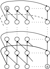

Figure 7: Instances structure of Simple Path and Related (left) and of Conformant Plan Checking (right) - •
Related: Given a genealogy graph storing information about relationships (father/brother) among people and given two people and , is an ancestor of ? The instances are encoded by facts when is known to be related to , that is, when is the father or a brother of . The problem can be encoded by the program
and the query is . The structure of the “genealogy” graph is the same as the one presented in [33] and coincides with the one used for testing Simple Path. Also in this case, the instances are generated by varying the number of nodes (thus the number of persons in the genealogy) of the graph.
- •
Strategic Companies: This is a slight variant of the problem domain used in the running example. The description here is of the problem as posed in the Third ASP Competition. We consider a collection of companies, where each company produces some goods in a set and each company is controlled by a set of owner companies . A subset of the companies is a strategic set if it is a minimal set of companies producing all the goods in , such that if for some then must hold. As in the Second Answer Set Competition,99 9 http://www.cs.kuleuven.be/~dtai/events/ASP-competition/index.shtml we assume that each product is produced by at most four companies, and that each company is controlled by at most four companies (the complexity of the problem under these restrictions is as hard as without them). Given two distinct companies , is there a strategic set of which contains both and ? The instances are encoded by facts when product is produced by companies and ; if is produced by fewer than four companies (but at least one), then contains repetitions of companies. Moreover, facts represent that company is controlled by companies and ; again, if is controlled by fewer than four companies, then contains repetitions. The problem can be encoded by the program
with the query . While the language presented in the previous sections allowed only for one atom in a query for simplicity, the implementation in DLV allows for a conjunction in a query; it is easy to see that a conjunctive query can be emulated by a rule with the conjunction in the body and an atom with a new predicate in the head, which contains all body arguments, and finally replacing the query conjunction with this atom. In this case this would mean adding a rule and replacing the query by . For this benchmark we used the instances submitted for the Second Answer Set Competition.
- •
Conformant Plan Checking: In addition, we have included a benchmark problem, which highlights the fact that our Magic Set technique can yield improvements not only for the grounding, but also for the model generation phase, as discussed in Section 7. This problem is inspired by a setting in planning, in particular testing whether a given plan is conformant with respect to a state transition diagram [30]. Such a diagram is essentially a directed graph formed of nodes representing states, and in which arcs are labeled by actions, meaning that executing the action in the source state will lead to the target state. In the considered setting nondeterminism is allowed, that is, executing an action in one state might lead nondeterministically to one of several successor states. A plan is a sequence of actions, and it is conformant with respect to a given initial state and a goal state if each possible execution of the action sequence leads to the goal state.
In our benchmark, we assume that the action selection process has already been done, thus having reduced the state transition diagram to those transitions that actually occur when executing the given plan. Furthermore we assume that there are exactly two possible non-goal successor states for any given state. This can also be viewed as whether all outgoing paths of a node in a directed graph reach a particular confluence node. We encoded instances by facts meaning that one of states and will be reached in the plan execution starting from . The problem is encoded using
and the query , where is the initial state and the goal state. If the query is cautiously true, the plan is conformant. The transition graphs in our experiments have the shape of a binary tree rooted in state , and from each leaf there is an arc to state , as depicted in Figure 7.
In addition, we have performed further experiments on an application scenario modeled from real-world data for answering user queries in a data integration setting. These latter experiments will be discussed in more detail in Section 6.
5.2 Results and Discussion
The experiments have been performed on a 3GHz Intel® Xeon® processor system with 4GB RAM under the Debian 4.0 operating system with a GNU/Linux 2.6.23 kernel. The DLV prototype used has been compiled using GCC 4.3.3. For each instance, we have allowed a maximum running time of 600 seconds (10 minutes) and a maximum memory usage of 3GB.
On all considered problems, outperformed , even if does not include the rewriting time, as discussed in Section 5.1. Let us analyze the results for each problem in more detail.
The results for Simple Path are reported in Figure 8. DLV without Magic Sets solves only the smallest instances, with a very steep increase in execution time. does better than DLV, but scales much worse than . The difference between and is mostly due to the grounding of the additional predicates that introduces.
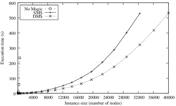
Figure 9 reports the results for Related. Compared to Simple Path, DLV without Magic Sets exhibits an even steeper increase in runtime, while in contrast both and scale better than on Simple Path. Comparing and , we note that appears to have an exponential speedup over . In this case, the computational gain of over is due to the dynamic optimization of the model search phase resulting from our Magic Sets definition. This aspect is better highlighted by the Conformant Plan Checking benchmark, and will be discussed later in this section.

For Strategic Companies, we report the results in Figure 10 as a bar diagram, because the instances do not have a uniform structure. The instances are, however, ordered by size. Also here, DLV without Magic Sets is clearly the least efficient of the tested systems, resolving only the smallest two instances in the allotted time (600 seconds). Concerning the other systems, and essentially show equal performance. In fact, the situation here is quite different to Simple Path and Related, because grounding the program produced by the Magic Set rewriting takes only a negligible amount of time for and . For this benchmark the important feature is reducing the ground program to the part which is relevant for the query, and we could verify that the ground programs produced by and are precisely the same.

Finally, the results for Conformant Plan Checking are shown in Figure 11. While DLV shows a similar behavior as for Simple Path and Related, here also does not scale well at all, and in fact appears to have an exponential speedup over . There is a precise reason for this: While the Magic Set rewriting of always creates a deterministic program defining the magic predicates, this is not true for . As a consequence, all magic predicates are completely evaluated during the grounding phase of DLV for , while for this is not the case. At the first glance, this may seem like a disadvantage of , as one might believe that the ground program becomes larger. However, it is actually a big advantage of , because it offers a more precise identification of the relevant part of the program. Roughly speaking, whatever identifies as relevant for the query will also be identified as relevant in , but can also include nondeterministic relevance information, which cannot. This means that in Magic Sets can be exploited also during the nondeterministic search phase of DLV, dynamically disabling parts of the ground program. In particular, after having made some choices, parts of the program may no longer be relevant to the query, but only because of these choices, and the magic atoms present in the ground program can render these parts satisfied, which means that they will no longer be considered in this part of the search. cannot induce any behavior like this and its effect is limited to the grounding phase of DLV, which can make a huge difference, as evidenced by Conformant Plan Checking.

5.3 Experimenting DMS with other Disjunctive Datalog Systems
In order to assess the effectiveness of on other systems than DLV, we tested the grounder Gringo [28] with the following solvers: ClaspD [21], Cmodels [46], GnT1 and GnT2 [37]. ClaspD is based on advanced Boolean constraint solving techniques, featuring backjumping and conflict-driven learning. Cmodels is based on the definition of program completion and loop formula for disjunctive programs [40, 47], and uses a SAT solver for generating candidate solutions and testing them. GnT1 is based on Smodels [61], a system handling Datalog programs with unstratified negation (normal programs): A disjunctive program is translated into a normal program, the stable models of which are computed by Smodels and represent stable model candidates of the original program. Each of these candidates is then checked to be a stable model of the original program by invoking Smodels on a second normal program. GnT2 is a variant of GnT1 in which the number of candidates produced by the first normal program is reduced by means of additional rules that discard unsupported models, i.e., models containing some atom for which there is no rule such that is true and is the only true atom in .
All of the benchmarks presented in the previous section were tested on these systems. Since is not implemented in these systems, rewritten programs were produced by DLV during the preparation of the experiment. We recall that does not depend on EDB relations and point out that DLV computes rewritten programs for the considered encodings in 1-2 hundredths of a second. The results of our experiment are reported in Figures 12–16. In general, we tried use a consistent scales in the graphs in order to ease comparability. However, for some graphs we chose a different scale in order to keep them readable for the main purpose (comparing performances with and without ), and we mention this explicitly in the accompanying text.

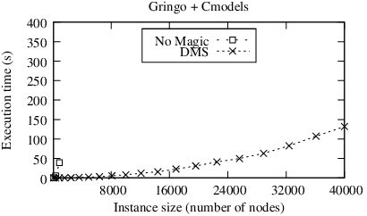


Concerning Simple Path, the advantages of over the unoptimized encoding are evident on all tested systems. In fact, as shown in Figure 12, without all tested systems did not answered in the allotted time (600 seconds) on instances with more than 400 nodes (900 for Cmodels). On the other hand, all of the instances considered in the benchmark (up to 40 thousands of nodes) were solved by all tested solvers with the encoding. We also observe that with the tested systems are faster than DLV in this benchmark, which is a clear indication of the optimization potential that can be provided to these systems by our Magic Set technique.


For Related we obtained a similar result, reported in Figure 13 (we used a different scale for the y-axis for Cmodels for readability). Without only the smallest instances were solved in the allotted time (up to 2025 nodes for ClaspD and Cmodels, up to 625 nodes for GnT1 and GnT2). With , instead, all tested systems solved the biggest instances of the benchmark (up to 10 thousands of nodes). In particular, with Cmodels is as performant as DLV in this benchmark.


The effectiveness of is also evident in the Strategic Companies benchmark (Figures 14–15). In fact, we observed sensible performance gains of all systems on all tested instances. GnT1, which is already faster than the other tested systems in this benchmark, draws particular advantage from , solving all instances in few seconds. We give another evidence of the optimization potential provided by to these systems by comparing the number of solved instances: Of a total of 60 tests, we counted 37 timeouts on the unoptimized encoding (10 on ClaspD, 14 on Cmodels, 3 on GnT1 and 10 on GnT2), while just one on the encoding obtained by applying . We point out that the timeout on the rewritten program was obtained by the Cmodels system, which alone collected 14 timeouts on the unoptimized encoding and is thus the least performant on this benchmark.


Finally, consider the results for Conformant Plan Checking reported in Figure 16 (we used a different scale on the y-axis for ClaspD for readability; note also that ClaspD and GnT2 only solved the smallest instances of this benchmark, and we thus used a different scale for their x-axes). The performance of ClaspD is poor in this benchmark, nonetheless we observed a slight improvement in execution time if is applied on the encoding reported in Section 5.1. Cmodels performs better than ClaspD in this case and the optimization potential of emerges with an exponential improvement in performance. A similar result was observed for GnT1, while GnT2 on this benchmark is the only outlier of the experiment: Its performance deteriorates if the original program is processed by . However, in this benchmark GnT2 performs worse that GnT1 also with the original encoding. In fact, while GnT1 solved the biggest instance (more than 65 thousands of states) in 209.74 seconds (12.28 seconds with the encoding), the execution of GnT2 did not terminate in the allotted time (600 seconds) on instances containing more than 10 thousands of states. We finally note that with GnT1 and Cmodels are faster than DLV in this benchmark. In fact, for the biggest instance in the benchmark, GnT1 and Cmodels required 12.28 and 19.13 seconds, respectively, while DLV terminated in 279.41 seconds. The significant performance gain of GnT1 and Cmodels due to is a further confirmation of the potential of our optimization technique.
6 Application to Data Integration
In this section we give a brief account of a case study that evidences the impact of the Magic Set method when used on programs that realize data integration systems. We first give an overview of data integration systems, show how they can be implemented using Datalog, and finally assess the impact of Magic Sets on a data integration system involving real-world data.
6.1 Data Integration Systems in a Nutshell
The main goal of data integration systems is to offer transparent access to heterogeneous sources by providing users with a global schema, which users can query without having to know from what sources the data come from. In fact, it is the task of the data integration system to identify and access the data sources which are relevant for finding the answer to a query over the global schema, followed by a combination of the data thus obtained. The data integration system uses a set of mapping assertions, which specify the relationship between the data sources and the global schema. Following [41], we formalize a data integration system as a triple , where:
- 1.
is the global (relational) schema, that is, a pair , where is a finite set of relation symbols, each with an associated positive arity, and is a finite set of integrity constraints (ICs) expressed on the symbols in . ICs are first-order assertions that are intended to be satisfied by database instances.
- 2.
is the source schema, constituted by the schemas of the various sources that are part of the data integration system. We assume that is a relational schema of the form , which means that there are no integrity constraints on the sources. This assumption implies that data stored at the sources are locally consistent; this is a common assumption in data integration, because sources are in general external to the integration system, which is not in charge of analyzing or restoring their consistency.
- 3.
is the mapping which establishes the relationship between and . In our framework, the mapping follows the GAV approach, that is, each global relation is associated with a view—a Datalog query over the sources.
The main semantic issue in data integration systems is that, since integrated sources are originally autonomous, their data, transformed via the mapping assertions, may not satisfy the constraints of the global schema. An approach to remedy to this problem that has lately received a lot of interest in the literature (see, e.g., [3, 11, 12, 14, 16, 17, 18, 19, 25, 26]) is based on the notion of repair for an inconsistent database as introduced in [4]. Roughly speaking, a repair of a database is a new database that satisfies the constraints in the schema, and minimally differs from the original one. Since an inconsistent database might possess multiple repairs, the standard approach in answering user queries is to return those answers that are true in every possible repair. These are called consistent answers in the literature.
6.2 Consistent Query Answering via Datalog Queries
There is an intuitive relation between consistent answers to queries over data integration systems and queries over Datalogprograms: Indeed, if one could find a translation from data sources, mapping, and the query to a Datalog program, which possesses a stable model for each possible repair, and a query over it, the consistent answers within the data integration system will correspond to cautious consequences of the obtained Datalog setting.
In fact, various authors [5, 7, 14, 16, 17, 31] considered the idea of encoding the constraints of the global schema into various kinds of logic programs, such that the stable models of this program yield the repairs of the database retrieved from the sources. Some of these approaches use logic programs with unstratified negation, [16], whereas disjunctive Datalog programs together with unstratified negation have been considered in [13, 51].
It has already been realized earlier that Magic Sets are a crucial optimization technique in this context, and indeed the availability of the transformational approach using stable logic programming as its core language was a main motivation for the research presented in this article, since in this way a Magic Set method for stable logic programs immediately yields an optimization technique for data integration systems. Indeed, the benefits of Magic Sets in the context of optimizing logic programs with unstratified negation (but without disjunction) have been discussed in [24]. The Magic Set technique defined in [24] is quite different from the one defined in this article, as it does not consider disjunctive rules, and works only for programs, which are consistent, that is, have at least one stable model. In [51] our preliminary work reported in [20], which eventually led to the present article, has been expanded in an ad-hoc way to particular kinds of Datalog programs with disjunction and unstratified negation. It is ad-hoc in the sense that it is tailored to programs which are created by the transformation described in [51]. The experimental results reported in [51] show huge computational advantages when using Magic Sets.
We now report an alternative transformation which produces Datalog programs (therefore different to [51], there are no unstratified occurrences of negation). This rewriting has been devised and used within the INFOMIX system on data integration [42].
Let be a data integration system where , and let be a database for , which is represented as a set of facts over the relational predicates in . We assume that constraints over the global schema are key and exclusion dependencies. In particular, we recall that a set of attributes is a key for the relation if:
and that an exclusion dependency holds between a set of attributes of a relation and a set of attributes of a relation if
Then, the disjunctive rewriting of a query with respect to is the Datalog program where:
- •
For each relation in and for each key defined over its set of attributes , contains the rules:
where , and .
- •
For each exclusion dependency between a set of attributes of a relation and a set of attributes of a relation , contains the following rule:
where , and . In the implementation the following equivalent rule is used:
- •
For each relation in , contains the rule:
- •
For each Datalog rule in such that:
where is a relation in and (for ) is a relation in , contains the rule:
It can be shown that for each user query (over ) and for each source database (over ), consistent query answers to precisely coincide with the set . Actually, within the INFOMIX project also inclusion dependencies have been considered according to the rewriting discussed in [16], whose details we omit for clarity. Since the rewriting for inclusion dependencies also modifies queries, in the INFOMIX project queries have been limited to conjunctive queries. It is however important to notice that the program contains only stratified negation and is therefore a Datalog program, making the Magic Set method defined in this article applicable.
6.3 Experimental Results
The effectiveness of the Magic Set method in this crucial application context has then been assessed via a number of experiments carried out on the demonstration scenario of the INFOMIX project, which refers to the information system of the University “La Sapienza” in Rome. The global schema consists of 14 global relations with 29 constraints, while the data sources include 29 relations of 3 legacy databases and 12 wrappers generating relational data from web pages. This amounts to more than 24MB of data regarding students, professors and exams in several faculties of the university. For a detailed description of the INFOMIX project see https://www.mat.unical.it/infomix/.
On this schema, we have tested five typical queries with different characteristics, which model different use cases. For the sake of completeness, the full encodings of the tested queries are reported in the Appendix. In particular, we measured the average execution time of DLV computing and on datasets of increasing size. The experiments were performed by running the INFOMIX prototype system on a 3GHz Intel® Xeon® processor system with 4GB RAM under the Debian 4.0 operating system with a GNU/Linux 2.6.23 kernel. The DLV prototype used as the computational core of the INFOMIX system had been compiled using GCC 4.3.3. For each instance, we allowed a maximum running time of 10 minutes and a maximum memory usage of 3GB.


The results, reported in Figure 17, confirm that on these typical queries the performance is considerably improved by Magic Sets. On Queries 1 to 4 in Figure 17 the response time scales much better with Magic Sets than without, appearing essentially linear on the tested instance sizes, while without Magic Sets the behavior has a decidedly non-linear appearance. We also observe that there is basically no improvement on Query . We have analyzed this query and for this use case all data seems to be relevant to the query, which means that Magic Sets cannot have any positive effect. It is however important to observe that the Magic Set rewriting does not incur any significant overhead.
7 Related Work
In this section we first discuss the main body of work which is related to , the technique developed in this paper for query answering optimization. In particular, we discuss Magic Set techniques for Datalog languages. The discussion is structured in paragraphs grouping techniques which cover the same language. After that, we discuss some applications for which have already been exploited. All these applications refer to the preliminary work published in [20].
Magic Sets for Datalog.
In order to optimize query evaluation in bottom-up systems, like deductive database systems, several works have proposed the simulation of top-down strategies by means of suitable transformations introducing new predicates and rewriting clauses. Among them, Magic Sets for Datalog queries are one of the best known logical optimization techniques for database systems. The method, first developed in [6], has been analyzed and refined by many authors; see, for instance, [9, 55, 62, 63]. These works form the foundations of .
Magic Sets for Datalog.
Many authors have addressed the issue of extending the Magic Set technique in order to deal with Datalog queries involving stratified negation. The main problem related to the extension of the technique to Datalog programs is how to assign a semantics to the rewritten programs. Indeed, while Datalog programs have a natural and accepted semantics, namely the perfect model semantics [2, 64], the application of Magic Sets can introduce unstratified negation in the rewritten programs. A solution has been presented in [10, 38, 39, 59]. In particular, in [38, 59] rewritten programs have been evaluated according to the well-founded semantics, a three-valued semantics for Datalog¬ programs which is two-valued for stratified programs, while in [10, 39] ad-hoc semantics have been defined. All of these methods exploit a property of Datalog which is not present in disjunctive Datalog, uniqueness of the intended model. This property in turn implies that query answering just consists in establishing the truth value of some atoms in one intended model. Using our terminology, brave and cautious reasoning coincide for these programs. Therefore, all these methods are quite different from , the technique developed in this paper.
Magic Sets for Datalog¬.
Extending the Magic Set technique to Datalog¬ programs must face two major difficulties. First, for a Datalog¬ program uniqueness of the intended model is no more guaranteed, thus query answering in this setting involves a set of stable models in general. The second difficulty is that parts of a Datalog¬ program may act as constraints, thus impeding a relevant interpretation to be a stable model. In [24] a Magic Set method for Datalog¬ programs has been defined and proved to be correct for coherent programs, i.e., programs admitting at least one stable model. This method takes special precautions for relevant parts of the program that act as constraints, called dangerous rules in [24]. We observe that dangerous rules cannot occur in Datalog programs, which allows for the simpler algorithm to work correctly for this class of programs.
Magic Sets for Datalog∨.
The first extension of the Magic Set technique to disjunctive Datalog is due to [32, 33], where the method has been presented and proved to be correct for Datalog∨ programs. We point out that the main drawback of this method is the introduction of collecting predicates. Indeed, magic and collecting predicates of have deterministic definitions. As a consequence, their extension can be completely computed during program instantiation, which means that no further optimization is provided for the subsequent stable model search. Moreover, while the correctness of has been formally established for Datalog programs in general, the applicability of to Datalog programs has only been outlined in [32, 33].
Applications.
Magic Sets have been applied in many contexts. In particular, [13, 36, 51, 53] have profitably exploited the optimization provided by . In particular, in [13, 51] a data integration system has been presented. The system is based on disjunctive Datalog and exploits for fast query answering. In [36, 53], instead, an algorithm for answering queries over description logic knowledge bases has been presented. More specifically, the algorithm reduces a knowledge base to a disjunctive Datalog program, so that can be exploited for query answering optimization.
8 Conclusion
The Magic Set method is one of the best-known techniques for the optimization of positive recursive Datalog programs due to its efficiency and its generality. Just a few other focused methods such as the supplementary Magic Set and other special techniques for linear and chain queries have gained similar visibility (see, e.g., [34, 56, 63]). After seminal papers [6, 9], the viability of the approach was demonstrated e.g., in [35, 55]. Later on, extensions and refinements were proposed, addressing e.g., query constraints in [62], the well-founded semantics in [38], or integration into cost-based query optimization in [60]. The research on variations of the Magic Set method is still going on. For instance, in [24] an extension of the Magic Set method was discussed for the class of unstratified logic programs (without disjunction). In [10] a technique for the class of soft-stratifiable programs was given. Finally, in [33] the first variant of the technique for disjunctive programs () was described.
In this paper, we have elaborated on the issues addressed in [32, 33]. Our approach is similar to , but differs in several respects:
- •
is a dynamic optimization of query answering, in the sense that in addition to the optimization of the grounding process (which is the only optimization performed by ), can drive the model generation phase by dynamically disabling parts of the program that become irrelevant in the considered partial interpretations.
- •
has a strong relationship with unfounded sets, allowing for a clean application to disjunctive Datalog programs also in presence of stratified negation.
- •
can be further improved by performing a subsequent subsumption check.
- •
is integrated into the DLV system [43], profitably exploiting the DLV internal data-structures and the ability of controlling the grounding module.
We have conducted experiments on several benchmarks, many of which taken from the literature. The results of our experimentation evidence that our implementation outperforms in general, often by an exponential factor. This is mainly due to the optimization of the model generation phase, which is specific to our Magic Set technique. In addition, we have conducted further experiments on a real application scenario, which show that Magic Sets can play a crucial role in optimizing consistent query answering over inconsistent databases. Importantly, other authors have already recognized the benefits of our optimization strategies with respect to this very important application domain [51], thereby confirming the validity and the robustness of the work discussed in this paper.
We conclude by observing that it has been noted in the literature (e.g., in [38]) that in the non-disjunctive case memoing techniques lead to similar computations as evaluations after Magic Set transformations. Also in the disjunctive case such techniques have been proposed (e.g., Hyper Tableaux [8]), for which similar relations might hold. While [38] has already evidenced that an advantage of Magic Sets over such methods is that they may be more easily combined with other optimization techniques, we believe that achieving a deeper comprehension of the relationships among these techniques constitutes an interesting avenue for further research.
Another issue that we leave for future work is to study the impact of changing some parameters of the method, in particular the impact of different SIPSes.
References
- [1] Serge Abiteboul, Richard Hull, and Victor Vianu. Foundations of Databases. Addison-Wesley, 1995.
- [2] Krzysztof R. Apt, Howard A. Blair, and Adrian Walker. Towards a Theory of Declarative Knowledge. In Minker [52], pages 89–148.
- [3] Marcelo Arenas, Leopoldo Bertossi, and Jan Chomicki. Scalar aggregation in fd-inconsistent databases. In International Conference on Database Theory (ICDT-2001), pages 39–53. Springer Verlag, 2001.
- [4] Marcelo Arenas, Leopoldo E. Bertossi, and Jan Chomicki. Consistent query answers in inconsistent databases. In Proc. of the 18th ACM SIGACT SIGMOD SIGART Symp. on Principles of Database Systems (PODS’99), pages 68–79, 1999.
- [5] Marcelo Arenas, Leopoldo E. Bertossi, and Jan Chomicki. Specifying and querying database repairs using logic programs with exceptions. In Proc. of the 4th Int. Conf. on Flexible Query Answering Systems (FQAS 2000), pages 27–41. Springer, 2000.
- [6] François Bancilhon, David Maier, Yehoshua Sagiv, and Jeffrey D. Ullman. Magic Sets and Other Strange Ways to Implement Logic Programs. In Proc. Int. Symposium on Principles of Database Systems, pages 1–16, 1986.
- [7] Pablo Barceló and Leopoldo Bertossi. Repairing databases with annotated predicate logic. In Proc. the 10th Int. Workshop on Non-Monotonic Reasoning (NMR 2002), pages 160–170, 2002.
- [8] Peter Baumgartner, Ulrich Furbach, and Ilkka Niemelä. Hyper Tableaux. In Proceedings of the European Workshop on Logics in Artificial Intelligence (JELIA’96), number 1126 in LNCS, pages 1–17. Springer, 1996.
- [9] Catriel Beeri and Raghu Ramakrishnan. On the power of magic. Journal of Logic Programming, 10(1–4):255–259, 1991.
- [10] Andreas Behrend. Soft stratification for magic set based query evaluation in deductive databases. In PODS ’03: Proceedings of the twenty-second ACM SIGMOD-SIGACT-SIGART symposium on Principles of database systems, pages 102–110, New York, NY, USA, 2003. ACM.
- [11] Leo Bertossi and Jan Chomicki. Query answering in inconsistent databases. In J. Chomicki, R. van der Meyden, and G. Saake, editors, Logics for Emerging Applications of Databases, chapter 2, pages 43–83. Springer-Verlag, 2003.
- [12] Leopoldo Bertossi, Jan Chomicki, Alvaro Cortes, and Claudio Gutierrez. Consistent answers from integrated data sources. In Proc. of the 6th Int. Conf. on Flexible Query Answering Systems (FQAS 2002), pages 71–85, 2002.
- [13] Leopoldo E. Bertossi and Loreto Bravo. Consistent query answers in virtual data integration systems. In Inconsistency Tolerance, volume 3300 of LNCS, pages 42–83. Springer, 2005.
- [14] Loreto Bravo and Leopoldo Bertossi. Logic programming for consistently querying data integration systems. In Proc. of the 18th Int. Joint Conf. on Artificial Intelligence (IJCAI 2003), pages 10–15, 2003.
- [15] Marco Cadoli, Thomas Eiter, and Georg Gottlob. Default Logic as a Query Language. IEEE Transactions on Knowledge and Data Engineering, 9(3):448–463, May/June 1997.
- [16] Andrea Calì, Domenico Lembo, and Riccardo Rosati. Query rewriting and answering under constraints in data integration systems. In Proc. of the 18th Int. Joint Conf. on Artificial Intelligence (IJCAI 2003), pages 16–21, 2003.
- [17] Jan Chomicki and Jerzy Marcinkowski. Minimal-change integrity maintenance using tuple deletions. Information and Computation, 197(1-2):90–121, 2005.
- [18] Jan Chomicki, Jerzy Marcinkowski, and Slawomir Staworko. Computing consistent query answers using conflict hypergraphs. In Proc. 13th ACM Conference on Information and Knowledge Management (CIKM-2004), pages 417–426. ACM Press, 2004.
- [19] Jan Chomicki, Jerzy Marcinkowski, and Slawomir Staworko. Hippo: A System for Computing Consistent Answers to a Class of SQL Queries. In Elisa Bertino, Stavros Christodoulakis, Dimitris Plexousakis, Vassilis Christophides, Manolis Koubarakis, Klemens Böhm, and Elena Ferrari, editors, 9th International Conference on Extending Database Technology (EDBT-2004), volume 2992 of Lecture Notes in Computer Science, pages 841–844. Springer, 2004.
- [20] Chiara Cumbo, Wolfgang Faber, Gianluigi Greco, and Nicola Leone. Enhancing the magic-set method for disjunctive datalog programs. In Proceedings of the the 20th International Conference on Logic Programming – ICLP’04, volume 3132 of Lecture Notes in Computer Science, pages 371–385, 2004.
- [21] Christian Drescher, Martin Gebser, Torsten Grote, Benjamin Kaufmann, Arne König, Max Ostrowski, and Torsten Schaub. Conflict-Driven Disjunctive Answer Set Solving. In Gerhard Brewka and Jérôme Lang, editors, Proceedings of the Eleventh International Conference on Principles of Knowledge Representation and Reasoning (KR 2008), pages 422–432, Sydney, Australia, 2008. AAAI Press.
- [22] Thomas Eiter, Georg Gottlob, and Heikki Mannila. Disjunctive Datalog. ACM Transactions on Database Systems, 22(3):364–418, September 1997.
- [23] Wolfgang Faber. Enhancing Efficiency and Expressiveness in Answer Set Programming Systems. PhD thesis, Institut für Informationssysteme, Technische Universität Wien, 2002.
- [24] Wolfgang Faber, Gianluigi Greco, and Nicola Leone. Magic Sets and their Application to Data Integration. Journal of Computer and System Sciences, 73(4):584–609, 2007.
- [25] Ariel Fuxman, Elham Fazli, and Renée J. Miller. Conquer: Efficient management of inconsistent databases. In SIGMOD Conference, 2005.
- [26] Ariel Fuxman and Renée J. Miller. First-order query rewriting for inconsistent databases. In Thomas Eiter and Leonid Libkin, editors, Proceedings of the 10th International Conference on Database Theory (ICDT 2005), number 3363 in LNCS, pages 337–351. Springer, 2005.
- [27] Michael R. Garey and David S. Johnson. Computers and Intractability, A Guide to the Theory of NP-Completeness. W.H. Freeman and Company, 1979.
- [28] Martin Gebser, Torsten Schaub, and Sven Thiele. Gringo : A new grounder for answer set programming. In Chitta Baral, Gerhard Brewka, and John Schlipf, editors, Logic Programming and Nonmonotonic Reasoning — 9th International Conference, LPNMR’07, volume 4483 of Lecture Notes in Computer Science, pages 266–271, Tempe, Arizona, May 2007. Springer Verlag.
- [29] M. Gelfond and V. Lifschitz. The Stable Model Semantics for Logic Programming. In Logic Programming: Proceedings Fifth Intl Conference and Symposium, pages 1070–1080, Cambridge, Mass., 1988. MIT Press.
- [30] R. Goldman and M. Boddy. Expressive Planning and Explicit Knowledge. In Proceedings AIPS-96, pages 110–117. AAAI Press, 1996.
- [31] Gianluigi Greco, Sergio Greco, and Ester Zumpano. A logic programming approach to the integration, repairing and querying of inconsistent databases. In Proc. of the 17th Int. Conf. on Logic Programming (ICLP’01), volume 2237 of Lecture Notes in Artificial Intelligence, pages 348–364. Springer, 2001.
- [32] Sergio Greco. Optimization of Disjunction Queries. In Danny De Schreye, editor, Proceedings of the 16th International Conference on Logic Programming (ICLP’99), pages 441–455, Las Cruces, New Mexico, USA, November 1999. The MIT Press.
- [33] Sergio Greco. Binding Propagation Techniques for the Optimization of Bound Disjunctive Queries. IEEE Transactions on Knowledge and Data Engineering, 15(2):368–385, March/April 2003.
- [34] Sergio Greco, Domenico Saccà, and Carlo Zaniolo. The PushDown Method to Optimize Chain Logic Programs (Extended Abstract). In Proc. Int. Colloquim on Automata, Languages and Programming, pages 523–534, 1995.
- [35] Ashish Gupta and Inderpal Singh Mumick. Magic-sets Transformation in Nonrecursive Systems. In Proceedings of the Thirteenth ACM SIGACT SIGMOD-SIGART Symposium on Principles of Database Systems (PODS-92), pages 354–367, 1992.
- [36] Ullrich Hustadt, Boris Motik, and Ulrike Sattler. Reasoning in description logics by a reduction to disjunctive datalog. Journal of Automated Reasoning, 39(3):351–384, 2007.
- [37] Tomi Janhunen, Ilkka Niemelä, Dietmar Seipel, Patrik Simons, and Jia-Huai You. Unfolding Partiality and Disjunctions in Stable Model Semantics. ACM Transactions on Computational Logic, 7(1):1–37, January 2006.
- [38] David B. Kemp, Divesh Srivastava, and Peter J. Stuckey. Bottom-up evaluation and query optimization of well-founded models. Theoretical Computer Science, 146:145–184, July 1995.
- [39] Jean-Marc Kerisit and Jean-Marc Pugin. Efficient query answering on stratified databases. In FGCS, pages 719–726, 1988.
- [40] Joohyung Lee and Vladimir Lifschitz. Loop Formulas for Disjunctive Logic Programs. In Proceedings of the Nineteenth International Conference on Logic Programming (ICLP-03). Springer Verlag, December 2003.
- [41] Maurizio Lenzerini. Data integration: A theoretical perspective. In Proc. of the 21st ACM SIGACT SIGMOD SIGART Symp. on Principles of Database Systems (PODS 2002), pages 233–246, 2002.
- [42] Nicola Leone, Georg Gottlob, Riccardo Rosati, Thomas Eiter, Wolfgang Faber, Michael Fink, Gianluigi Greco, Giovambattista Ianni, Edyta Kałka, Domenico Lembo, Maurizio Lenzerini, Vincenzino Lio, Bartosz Nowicki, Marco Ruzzi, Witold Staniszkis, and Giorgio Terracina. The INFOMIX System for Advanced Integration of Incomplete and Inconsistent Data. In Proceedings of the 24th ACM SIGMOD International Conference on Management of Data (SIGMOD 2005), pages 915–917, Baltimore, Maryland, USA, June 2005. ACM Press.
- [43] Nicola Leone, Gerald Pfeifer, Wolfgang Faber, Thomas Eiter, Georg Gottlob, Simona Perri, and Francesco Scarcello. The DLV System for Knowledge Representation and Reasoning. ACM Transactions on Computational Logic, 7(3):499–562, July 2006.
- [44] Nicola Leone, Pasquale Rullo, and Francesco Scarcello. Disjunctive Stable Models: Unfounded Sets, Fixpoint Semantics and Computation. Information and Computation, 135(2):69–112, June 1997.
- [45] Senlin Liang, Paul Fodor, Hui Wan, and Michael Kifer. OpenRuleBench: An analysis of the performance of rule engines. In Juan Quemada, Gonzalo León, Yoëlle S. Maarek, and Wolfgang Nejdl, editors, Proceedings of the 18th International Conference on World Wide Web (WWW 2009), pages 601–610. ACM, 2009.
- [46] Yuliya Lierler. Disjunctive Answer Set Programming via Satisfiability. In Chitta Baral, Gianluigi Greco, Nicola Leone, and Giorgio Terracina, editors, Logic Programming and Nonmonotonic Reasoning — 8th International Conference, LPNMR’05, Diamante, Italy, September 2005, Proceedings, volume 3662 of Lecture Notes in Computer Science, pages 447–451. Springer Verlag, September 2005.
- [47] Fangzhen Lin and Yuting Zhao. ASSAT: Computing Answer Sets of a Logic Program by SAT Solvers. In Proceedings of the Eighteenth National Conference on Artificial Intelligence (AAAI-2002), Edmonton, Alberta, Canada, 2002. AAAI Press / MIT Press.
- [48] Jorge Lobo, Jack Minker, and Arcot Rajasekar. Foundations of Disjunctive Logic Programming. The MIT Press, Cambridge, Massachusetts, 1992.
- [49] Marco Manna, Massimo Ruffolo, Ermelinda Oro, Mario Alviano, and Nicola Leone. The HiLeX system for semantic information extraction. Transactions on Large-Scale Data- and Knowledge-Centered Systems. Springer Berlin/Heidelberg, Lecture Notes in Computer Science 7100:91–125, 2012.
- [50] Marco Manna, Francesco Scarcello, and Nicola Leone. On the complexity of regular-grammars with integer attributes. Journal of Computer and System Sciences (JCSS), 77(2):393–421, 2011.
- [51] Mónica Caniupán Marileo and Leopoldo E. Bertossi. The consistency extractor system: Querying inconsistent databases using answer set programs. In SUM 2007, pages 74–88, 2007.
- [52] Jack Minker, editor. Foundations of Deductive Databases and Logic Programming. Morgan Kaufmann Publishers, Inc., Washington DC, 1988.
- [53] Boris Motik. Reasoning in Description Logics using Resolution and Deductive Databases. PhD thesis, Fakultät für Wirtschaftswissenschaften, Universität Fridericiana zu Karlsruhe, 2006.
- [54] Boris Motik and Ulrike Sattler. A comparison of reasoning techniques for querying large description logic aboxes. In Miki Hermann and Andrei Voronkov, editors, Logic for Programming, Artificial Intelligence, and Reasoning, 13th International Conference (LPAR 2006), volume 4246 of Lecture Notes in Computer Science, pages 227–241. Springer, 2006.
- [55] Inderpal Singh Mumick, Sheldon J. Finkelstein, Hamid Pirahesh, and Raghu Ramakrishnan. Magic is relevant. In Proceedings of the 1990 ACM SIGMOD International Conference on Management of Data, pages 247–258, 1990.
- [56] Raghu Ramakrishnan, Yehoshua Sagiv, Jeffrey D. Ullman, and Moshe Y. Vardi. Logical Query Optimization by Proof-Tree Transformation. Journal of Computer and System Sciences, 47(1):222–248, 1993.
- [57] Francesco Ricca, Mario Alviano, Antonella Dimasi, Giovanni Grasso, Salvatore Maria Ielpa, Salvatore Iiritano, Marco Manna, and Nicola Leone. A logic-based system for e-tourism. Fundamenta Informaticae. IOS Press, 105(1–2):35–55, 2010.
- [58] Francesco Ricca, Giovanni Grasso, Mario Alviano, Marco Manna, Vincenzino Lio, Salvatore Iiritano, and Nicola Leone. Team-building with answer set programming in the Gioia-Tauro seaport. Theory and Practice of Logic Programming, 2012. To appear, doi:10.1017/S147106841100007X.
- [59] K. A. Ross. Modular Stratification and Magic Sets for Datalog Programs with Negation. Journal of the ACM, 41(6):1216–1266, 1994.
- [60] Praveen Seshadri, Joseph M. Hellerstein, Hamid Pirahesh, T. Y. Cliff Leung, Raghu Ramakrishnan, Divesh Srivastava, Peter J. Stuckey, and S. Sudarshan. Cost-based optimization for magic: Algebra and implementation. In H. V. Jagadish and Inderpal Singh Mumick, editors, Proceedings of the 1996 ACM SIGMOD International Conference on Management of Data, pages 435–446. ACM Press, June 1996.
- [61] Patrik Simons, Ilkka Niemelä, and Timo Soininen. Extending and Implementing the Stable Model Semantics. Artificial Intelligence, 138:181–234, June 2002.
- [62] Peter J. Stuckey and S. Sudarshan. Compiling query constraints. In Proceedings of the Thirteenth Symposium on Principles of Database Systems (PODS’94), pages 56–67. ACM Press, May 1994.
- [63] Jeffrey D. Ullman. Principles of Database and Knowledge-Base Systems, Volume II. Computer Science Press, 1989.
- [64] A. van Gelder. Negation as Failure Using Tight Derivations for General Logic Programs. In Minker [52], pages 1149–1176.
Appendix A Queries on the INFOMIX Demo Scenario
INFOMIX is a project that was funded by the European Commission in its Information Society Technologies track of the Sixth Framework Programme for providing an advanced system for information integration. A detailed description of the project, including references in the literature, can be found at https://www.mat.unical.it/infomix/. Five typical queries of the INFOMIX demo scenario have been considered for assessing Dynamic Magic Sets. The full encodings of the tested queries are reported in Figures 18–19. Note that the encodings include the transformation described in Section 6, and that underlined predicates denote source relations.