Skewed Multivariate Birnbaum–Saunders Distributions

The univariate family of distributions proposed by Birnbaum and Saunders (1969), also known as the fatigue life distributions, has been widely applied for describing fatigue lifetimes. This family was originally derived from a model for which failure follows from the development and growth of a dominant crack. A random variable $T$ has a Birnbaum–Saunders (BS) distribution if it can be written as $T=\beta\{\alpha Z/2+[(\alpha Z/2)^{2}+1]^{1/2}\}^{2}$, where $Z$ is a random variable following the standard normal distribution, i.e. $Z\sim{\rm N}(0,1)$. Its density function is

which depends on two parameters: the shape $\alpha>0$ and scale $\beta>0$, which is also the median of the distribution. We have $kT\sim{\rm BS}(\alpha,k\beta)$ for any $k>0$, i.e. the BS distribution is closed under scale transformations. The expected value, variance, skewness and kurtosis of $T$ are, respectively,

The density function (1) is right skewed and the skewness decreases with $\alpha$. Notice that both mean and variance increase as $\alpha$ increases. It is also of interest to mention that if $T\sim{\rm BS}(\alpha,\beta)$, then $T^{-1}\sim{\rm BS}(\alpha,\beta^{-1})$. It implies that the BS distribution also belongs to the family of random variables closed under reciprocation (Saunders, 1974). It then follows that

The shape of the hazard function of the BS distribution is discussed in Kundu et al. (2008). The authors showed that the hazard rate function is not monotone and is unimodal for all ranges of the parameter values. Some interesting results on improved statistical inference for the BS distribution may be revised in Wu and Wong (2004) and Lemonte et al. (2007); Lemonte et al. (2008).

The univariate BS distribution has received significant attention over the last few years by many researchers and some generalizations are proposed in Díaz–García and Leiva (2005), Owen (2006), Guiraud et al. (2009), Leiva et al. (2009), Castillo et al. (2011) and Cordeiro and Lemonte (2011), among other. On the other hand, as far as we know, little work has been done to extend the BS distribution to the multivariate case. We can refer to the works by Díaz–García and Domínguez–Molina (2006), Kundu et al. (2010) and Caro–Lopera et al. (2012). In Díaz–García and Domínguez–Molina (2006), the authors defined an independent multivariate BS distribution. By using the bivariate normal distribution function, Kundu et al. (2010) proposed a bivariate BS distribution which is absolutely continuous and has five parameters. Finally, Caro–Lopera et al. (2012) introduced the matrix-variate generalized BS distribution.

As can be observed, little work on multivariate versions for the BS distribution have been published. In this paper, in addition to the existing multivariate BS models, we shall propose the asymmetric (skewed) multivariate BS distribution based on the work of Arnold et al. (2002). The main motivation for introducing this multivariate version of the BS distribution relies on the fact that the practitioners will have a new multivariate BS model to use in multivariate settings, since the formulae related with the new multivariate model are manageable and with the use of modern computer resources and its numerical capabilities, the proposed model may prove to be an useful addition to the arsenal of applied statisticians. Additionally, the new model is quite flexible (see Figure 1 in Section 2) and can be widely applied in analyzing multivariate data. Further, we provide an application to real data in which is showed that the new multivariate model yields a better fit than other multivariate BS distributions available in the literature.

The paper unfolds as follows. The skewed bivariate BS distribution is defined in Section 2 and then several properties are discussed. The multivariate extension is presented in Section 3. In Section 4, we propose different methods for estimating the unknown parameters as well as derive the information matrix and discuss likelihood ratio tests for some hypotheses of interest. In particular, we propose modified moment estimators for the unknown parameters which are explicit in form and can therefore be used effectively as the initial guess in the iterative process for the computation of the maximum likelihood estimators. Further, the asymptotic distribution of the maximum likelihood estimators is derived and thus the asymptotic confidence intervals for the unknown parameters can be constructed. The usefulness of the proposed model is illustrated in an application to real data in Section 5. We also introduce in Section 6 the skewed bivariate generalized BS distribution. Finally, Section 7 closes the paper with some concluding remarks.

We initially consider the skewed bivariate BS distribution. For each $x\in\mathbb{R}$ and for each $y\in\mathbb{R}$, consider the conditional distributions

where $X|Y=y\sim{\rm SN}(\lambda y)$ means that given $Y=y$, $X|Y=y$ has skew normal distribution (Azzalini, 1985). The shape parameter $\lambda\in\mathbb{R}$ determines the skewness of the density. From Arnold et al. (2002) and using the conditional distributions in (2), the joint probability density function (pdf) of the random vector $(X,Y)$ takes the form

where $\phi(\cdot)$ and $\Phi(\cdot)$ denote the pdf and cumulative distribution function (cdf) of the standard normal distribution, respectively. Also, $f_{X}(x)=\phi(x)$ and $f_{Y}(y)=\phi(y)$. If $\lambda=0$ in (3), then $f_{X,Y}(x,y)=\phi(x)\phi(y)$ and hence $X$ and $Y$ become independent. For $\lambda\neq 0$, it can be shown that the correlation between $X$ and $Y$, $\rho(X,Y)$ say, is given by

where $U(a,b,z)$ denotes the confluent hypergeometric function, defined as

with $b>a>0$ and $z>0$, and $\Gamma(\cdot)$ represents the gamma function. Therefore, the parameter $\lambda$ also governs the correlation.

Let $Z_{j}\sim{\rm N}(0,1)$, for $j=1,2$, with $Z_{1}|Z_{2}=z_{2}\sim{\rm SN}(\lambda z_{2})$ and $Z_{2}|Z_{1}=z_{1}\sim{\rm SN}(\lambda z_{1})$. Then, taking the transformation

where $\alpha_{j}>0$ and $\beta_{j}>0$, the joint pdf of the skewed bivariate BS (SBVBS) distribution takes the form

where

The notation used is $(T_{1},T_{2})\sim{\rm SBVBS}(\alpha_{1},\alpha_{2},\beta_{1},\beta_{2},\lambda)$. The random variables $T_{1}$ and $T_{2}$ become independent for $\lambda=0$ in (4) and hence the proposed bivariate model reduces to the independent bivariate model considered by Díaz–García and Domínguez–Molina (2006). So, as remarked, the shape parameter $\lambda$ also introduces correlation between $T_{1}$ and $T_{2}$.

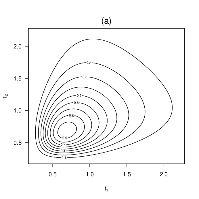
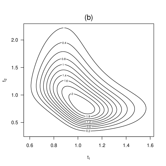
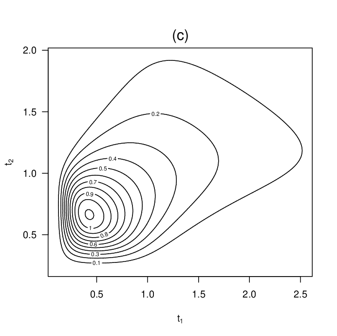
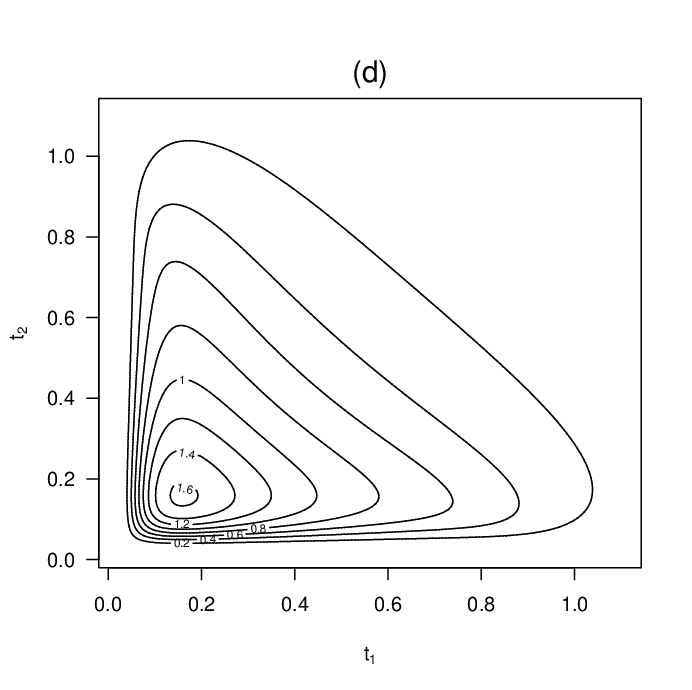
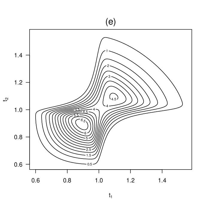
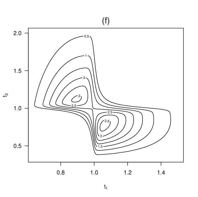
Contour plots for the joint pdf (4) are presented in Figure 1. From this figure, note that (4) can take on different shapes and will therefore be useful in analyzing bivariate data. Additionally, notice that (4) can be unimodal or bimodal depending on the value of $\lambda$.

The following theorem provides the marginal and conditional distributions of the SBVBS distribution.

Some properties of the random vector $(T_{1},T_{2})$ are provided in the following theorem.

Since the marginal distributions of the bivariate vector $(T_{1},T_{2})$ are BS distributions, the mean and variance of $T_{1}$ and $T_{2}$ are obtained directly from these marginals in the forms

Additionally,

The product moments of $(T_{1},T_{2})$, $\mathbb{E}(T_{1}^{r}T_{2}^{s})$ say, are very complicated to be determined algebraically and have to be computed numerically. In the following, we shall derive an expression for $\mathbb{E}(T_{1}T_{2})$ which can be of some interest. We can show after some algebra that

where

with

being $c_{1}=1$, $c_{2}=4\lambda^{2}/(3!)$ and $c_{3}=32\lambda^{4}/(5!)$. For $\lambda=0$ (independent case), we have immediately that

We have considered the bivariate case in Section 2, but extensions to higher dimension can be readily accomplished using suitable notation. For a random variable $\bm{Z}=(Z_{1},\ldots,Z_{p})^{\top}$ of dimension $p$, we define the subvectors $\bm{Z}_{(1)}$,…,$\bm{Z}_{(p)}$ of dimensions $(p-1)$ such that, for each $j=1,\ldots,p$, $\bm{Z}_{(j)}$ denotes the vector $\bm{Z}$ with the $j$th coordinate $Z_{j}$ deleted. Analogously, for a real vector $\bm{z}=(z_{1},\ldots,z_{p})^{\top}$, $\bm{z}_{(j)}$ is obtained from $\bm{z}$ with the $j$th coordinate $z_{j}$ deleted.

By assuming (for each $j=1,\ldots,p$) that

the joint pdf of $\bm{Z}=(Z_{1},\ldots,Z_{p})^{\top}$ takes the form (Arnold et al., 2002)

Thus, under the transformation

where $Z_{j}\sim{\rm N}(0,1)$, we obtain the joint pdf of $\bm{T}=(T_{1},\ldots,T_{p})^{\top}$ in the form

where $\alpha_{j}>0$, $\beta_{j}>0$ and $a_{j}$ is given in (5), $j=1,\ldots,p$. Let $\bm{\alpha}=(\alpha_{1},\ldots,\alpha_{p})^{\top}$ and $\bm{\beta}=(\beta_{1},\ldots,\beta_{p})^{\top}$. If $\bm{T}=(T_{1},\ldots,T_{p})^{\top}$ has skewed multivariate BS distribution, then we use the notation $\bm{T}\sim{\rm SMVBS}(\bm{\alpha},\bm{\beta},\lambda)$.

Several properties discussed in the bivariate case hold for this multivariate extension. For example, $T_{j}\sim{\rm BS}(\alpha_{j},\beta_{j})$ for $j=1,\ldots,p$, i.e. the marginal distributions are BS distributions; $\lambda=0$ corresponds to the independent case; for $k_{1},\ldots,k_{p}>0$, $(k_{1}T_{1},\ldots,k_{p}T_{p})\sim{\rm SMVBS}(\bm{\alpha},\bm{\beta}^{*},\lambda)$ with $\bm{\beta}^{*}=(k_{1}\beta_{1},\ldots,k_{p}\beta_{p})^{\top}$; $(T_{1}^{-1},\ldots,T_{p}^{-1})\sim{\rm SMVBS}(\bm{\alpha},\bm{\beta}^{**},\lambda)$, where $\bm{\beta}^{**}=(\beta_{1}^{-1},\ldots,\beta_{p}^{-1})^{\top}$, and so on. In the next section, we shall consider estimation for the unknown parameters of the ${\rm SMVBS}$ distribution in (6) as well as inference. Thus, from these general results the bivariate case considered in Section 2 can be easily specialized by considering $p=2$.

In this section, we address the problem of estimating the unknown parameters of the SMVBS distribution. Let $\bm{t}_{1},\ldots,\bm{t}_{n}$ denote a random sample of the ${\rm SMVBS}(\bm{\alpha},\bm{\beta},\lambda)$ distribution, where $\bm{t}_{i}=(t_{1i},\ldots,t_{pi})^{\top}$ and, as before, $\bm{\alpha}=(\alpha_{1},\ldots,\alpha_{p})^{\top}$ and $\bm{\beta}=(\beta_{1},\ldots,\beta_{p})^{\top}$. Let $\bm{\theta}=(\bm{\alpha}^{\top},\bm{\beta}^{\top},\lambda)^{\top}$ be the parameter vector of interest of dimension $2p+1$.

In this section, for illustrative purposes, we present an empirical application to demonstrate the applicability of the proposed skewed multivariate BS distribution. For the sake of comparison, we also consider the distributions proposed in Díaz–García and Domínguez–Molina (2006) and Kundu et al. (2010). We shall use the data set obtained from Volle (1985), which represent the amount of time (in hours) spent on two categories of activities over 100 days in the year 1976 for 28 individuals. The data are: (115, 175), (100, 115), (130, 160), (115, 180), (119, 143), (100, 150), (960, 132), (150, 115), (142, 870), (180, 125), (152, 122), (174, 119), (140, 100), (147, 840), (105, 700), (950, 600), (130, 600), (105, 800), (117, 650), (850, 400), (102, 450), (100, 960), (920, 640), (128, 860), (102, 122), (107, 730), (860, 580), (940, 580). The first figure represents the amount of time spent on eating and the second figure represents the amount of time spent on watching television. All the computations were done using the Ox matrix programming language (Doornik, 2006).

We now use the SBVBS distribution to model these bivariate data. We obtain from the data $\bar{s}_{1}=118.14$, $\bar{s}_{2}=99.43$, $\bar{r}_{1}=113.40$ and $\bar{r}_{2}=84.61$, and hence the MMEs are $\check{\alpha}_{1}=0.2035$, $\check{\alpha}_{2}=0.4099$, $\check{\beta}_{1}=115.7457$ and $\check{\beta}_{2}=91.7220$. These values are used as initial guesses for $\alpha_{1}$, $\alpha_{2}$, $\beta_{1}$ and $\beta_{2}$, respectively. An initial guess for $\lambda$ is also required to start the maximization of the log-likelihood function (8), i.e. to solve the likelihood equations (9) with $p=2$. As initial value for $\lambda$ we consider $\check{\lambda}=0$, which corresponds to the independent case. The algorithm converges after 21 steps and the MLEs of $\alpha_{1}$, $\alpha_{2}$, $\beta_{1}$, $\beta_{2}$ and $\lambda$ are $\widehat{\alpha}_{1}=0.2047$, $\widehat{\alpha}_{2}=0.4101$, $\widehat{\beta}_{1}=113.2907$, $\widehat{\beta}_{2}=90.7447$ and $\widehat{\lambda}=0.8806$, respectively. Notice that the MMEs for $\alpha_{1}$, $\alpha_{2}$, $\beta_{1}$ and $\beta_{2}$ are close to their respective MLEs. We have also considered other initial guesses for $\lambda$, for example, with the initial values $\check{\lambda}=-5,-2,3$ and 4, the algorithm converges to the same estimates after 39, 26, 25 and 31 steps, respectively. The 95% asymptotic confidence intervals for $\alpha_{1}$, $\alpha_{2}$, $\beta_{1}$, $\beta_{2}$ and $\lambda$ are (0.1508, 0.2586), (0.3051, 0.5152), (104.8325, 121.7489), (77.8975, 103.5919) and (0.0349, 1.7263), respectively.

Next, we make use of the LR statistic to test the null hypothesis $\mathcal{H}_{0}:\lambda=0$ against $\mathcal{H}_{1}:\lambda\neq 0$. Here, $\omega=2\{\ell(\widehat{\alpha}_{1},\widehat{\alpha}_{2},\widehat{\beta}_{1},\widehat{\beta}_{2},\widehat{\lambda})-\ell(\widetilde{\alpha}_{1},\widetilde{\alpha}_{2},\widetilde{\beta}_{1},\widetilde{\beta}_{2},0)\}$, where $\widetilde{\alpha}_{1}$, $\widetilde{\alpha}_{2}$, $\widetilde{\beta}_{1}$ and $\widetilde{\beta}_{2}$ are, respectively, the restricted MLEs of $\alpha_{1}$, $\alpha_{2}$, $\beta_{1}$ and $\beta_{2}$ obtained under $\mathcal{H}_{0}$ and are given by $\widetilde{\alpha}_{1}=0.2035$, $\widetilde{\alpha}_{2}=0.4099$, $\widetilde{\beta}_{1}=115.7470$ and $\widetilde{\beta}_{2}=91.7128$. By a little computation, we have that the LR test statistic ($\omega$) equals 6.6834 (p-value $<0.01$). Therefore, the null hypothesis $\mathcal{H}_{0}:\lambda=0$ is strongly rejected at the usual significance levels and hence the assumption of the skewness (correlation) is suitable for the current bivariate data. Since the bivariate distribution in Díaz–García and Domínguez–Molina (2006), DG–DM say, and our proposed model are nested models (i.e. the DG–DM model holds for $\lambda=0$), the null and alternative hypotheses can be rewritten as $\mathcal{H}_{0}$: DG–DM against $\mathcal{H}_{1}$: SBVBS. Thus, based on the LR statistic above, the SBVBS distribution fits the data better than the bivariate DG–DM model.

The generalized LR statistic ($T_{LR,NN}$) presented in Vuong (1989) can be used for discriminating among non-nested models, which is a distance between the two models measured in terms of the Kullback–Liebler information criterion. Then, our proposed model and the bivariate model in Kundu et al. (2010) can be compared by using $T_{LR,NN}$. For strictly nonnested models, $T_{LR,NN}$ converges in distribution to a standard normal distribution under the null hypothesis of equivalence of the models and the null hypothesis is not rejected if $|T_{LR,NN}|\leq z_{\gamma/2}$, where $z_{\gamma/2}$ is the quantile $100(1-\gamma/2)\%$ of the standard normal distribution. On the other hand, we reject at significance level $\gamma$ the null hypothesis of equivalence of the models in favor of the SBVBS model being better (or worse) than the model in Kundu et al. (2010) if $T_{LR,NN}>z_{\gamma}$ (or $T_{LR,NN}<-z_{\gamma}$). The generalized LR test statistic ($T_{LR,NN}$) equals $4.0903$ (p-value $<0.01$). Therefore, the proposed model is significantly better than the model in Kundu et al. (2010) according to the generalized LR statistic to model the current data.

References

• Abramowitz and Stegun (1970) Abramowitz, M., Stegun, I.A. (1970). Handbook of Mathematical Functions. National Bureau of Standards: Washington.
• Arnold et al. (2002) Arnold, B.C., Castilho, E., Sarabia, J.M. (2002). Conditionally specified multivariate skewed distributions. Sankhya A 64, 206–226.
• Azzalini (1985) Azzalini, A. (1985). A class of distributions which includes the normal ones. Scandinavian Journal of Statistics 12, 171–178.
• Birnbaum and Saunders (1969) Birnbaum, Z.W., Saunders, S.C. (1969). A new family of life distributions. Journal of Applied Probability 6, 319–327.
• Caro–Lopera et al. (2012) Caro–Lopera, F.J., Leiva, V., Balakrishnan, N. (2012). Connection between the Hadamard and matrix products with an application to matrix-variate Birnbaum–Saunders distributions. Journal of Multivariate Analysis 104, 126–139.
• Castillo et al. (2011) Castillo, N.O., Gómez, H.W., Bolfarine, H. (2011). Epsilon Birnbaum–Saunders distribution family: properties and inference. Statistical Papers 52, 871–883.
• Chen and Balakrishnan (1995) Chen, G., Balakrishnan, N. (1995). A general purpose approximate goodness-of-fit test. Journal of Quality Technology 27, 154–161.
• Cordeiro and Lemonte (2011) Cordeiro, G.M., Lemonte, A.J. (2011). The β\beta-Birnbaum–Saunders distribution: an improved distribution for fatigue life modeling. Computational Statistics and Data Analysis 55, 1445–1461.
• Cox and Hinkley (1974) Cox, D.R., Hinkley, D.V. (1974). Theoretical Statistics. Chapman and Hall: London.
• Díaz–García and Domínguez–Molina (2006) Díaz–García, J.A., Domínguez–Molina, J.R. (2006). Some generalisations of Birnbaum–Saunders and sinh–normal distributions. International Mathematical Forum 1, 1709–1727.
• Díaz–García and Leiva (2005) Díaz–García, J.A., Leiva, V. (2005). A new family of life distributions based on the elliptically contoured distributions. Journal of Statistical Planning and Inference 128, 445–457.
• Doornik (2006) Doornik, J.A. (2006). An Object-Oriented Matrix Language – Ox 4, 5th ed. Timberlake Consultants Press: London.
• Fang et al. (1990) Fang, K.T., Kotz, S., Ng, K.W. (1990). Symmetric Multivariate and Related Distributions. Chapman and Hall: London.
• Gradshteyn and Ryzhik (2007) Gradshteyn, I.S., Ryzhik, I.M. (2007). Table of Integrals, Series, and Products. Academic Press: New York.
• Guiraud et al. (2009) Guiraud, P., Leiva, V., Fierro, R. (2009). A non-central version of the Birnbaum–Saunders distribution for reliability analysis. IEEE Transactions on Reliability 58, 152–160.
• Gupta and Varga (1993) Gupta, A.K., Varga, T. (1993). Elliptically Contoured Models in Statistics. Kluwer Academic Publishers: Boston.
• Kundu et al. (2010) Kundu, D., Balakrishnan, N., Jamalizadeh, A. (2010). Bivariate Birnbaum–Saunders distribution and associated inference. Journal of Multivariate Analysis 101, 113–125.
• Kundu et al. (2008) Kundu, D., Kannan, N., Balakrishnan, N. (2008). On the hazard function of Birnbaum–Saunders distribution and associated inference. Computational Statistics and Data Analysis 52, 2692–2702.
• Leiva et al. (2008) Leiva, V., Barros, M., Paula, G.A., Sanhueza, A. (2008). Generalized Birnbaum–Saunders distributions applied to air pollutant concentration. Environmetrics 19, 235–249 .
• Leiva et al. (2009) Leiva, V., Sanhueza, A., Angulo, J.M. (2009). A length-biased version of the Birnbaum–Saunders distribution with application in water quality. Stochastic Environmental Research and Risk Assessment 23, 299–307.
• Lemonte et al. (2007) Lemonte, A.J., Cribari–Neto, F., Vasconcellos, K.L.P. (2007). Improved statistical inference for the two-parameter Birnbaum–Saunders distribution. Computational Statistics and Data Analysis 51, 4656–4681.
• Lemonte et al. (2008) Lemonte, A.J., Simas, A.B., Cribari–Neto, F. (2008). Bootstrap-based improved estimators for the two-parameter Birnbaum–Saunders distribution. Journal of Statistical Computation and Simulation 78, 37–49.
• Ng et al. (2003) Ng, H.K.T., Kundu, D., Balakrishnan, N. (2003). Modified moment estimation for the two-parameter Birnbaum–Saunders distribution. Computational Statistics and Data Analysis 43, 283–298.
• Owen (1956) Owen, D.B. (1956). Tables for computing bivariate normal probabilities. Annals of Mathematical Statistics 27, 1075–1090.
• Owen (2006) Owen, W.J. (2006). A new three-parameter extension to the Birnbaum–Saunders distribution. IEEE Transactions on Reliability 55, 475–479.
• R Development Core Team (2010) R Development Core Team (2010). R: A Language and Environment for Statistical Computing. R Foundation for Statistical Computing: Vienna, Austria.
• Saunders (1974) Saunders, S.C. (1974). A family of random variables closed under reciprocation. Journal of the American Statistical Association 69, 533–539.
• Volle (1985) Volle, M. (1985). Analyse des Données, 3rd ed. Economica: Paris.
• Vuong (1989) Vuong, Q.H. (1989). Likelihood ratio tests for model selection and non-nested hypotheses. Econometrica 57, 307–333.
• Wu and Wong (2004) Wu, J., Wong, A.C.M. (2004). Improved interval estimation for the two-parameter Birnbaum–Saunders distribution. Computational Statistics and Data Analysis 47, 809–821.