Quantum lump dynamics on the two-sphereThanks: E-mail: speight@maths.leeds.ac.uk
Abstract
It is well known that the low-energy classical dynamics of solitons of Bogomol’nyi type is well approximated by geodesic motion in , the moduli space of static -solitons. There is an obvious quantization of this dynamics wherein the wavefunction evolves according to the Hamiltonian , where is the Laplacian on . Born-Oppenheimer reduction of analogous mechanical systems suggests, however, that this simple Hamiltonian should receive corrections including , the scalar curvature of , and , the -soliton Casimir energy, which are usually difficult or impossible to compute, and whose effect on the energy spectrum is unknown. This paper analyzes the spectra of and two corrections to it suggested by work of Moss and Shiiki, namely and , in the simple but nontrivial case of a single lump moving on the two-sphere. Here , a noncompact kähler 6-manifold invariant under an action, whose geometry is well understood. The symmetry gives rise to two conserved angular momenta, spin and isospin. By exploiting the diffeomorphism , a hidden isometry of is found which implies that all three energy spectra are symmetric under spin-isospin interchange. The Casimir energy is found exactly on an submanifold of , using standard results from harmonic map theory and zeta function regularization, and approximated numerically on the rest of . The lowest 19 eigenvalues of are found, and their spin-isospin and parity compared for . It is found that the curvature corrections in lead to a qualitatively unchanged low-level spectrum while the Casimir energy in leads to significant changes. The scaling behaviour of the spectra under changes in the radii of the domain and target spheres is analyzed, and it is found that the disparity between the spectra of and is reduced when the target sphere is made smaller.
Version: November 1, 2012
1 Introduction
Many field theories arising naturally in theoretical high energy physics may be said to be of Bogomol’nyi type. For such theories there is a topological lower bound on the energy of field configurations, and this bound is attained only by solutions of a first order “self-duality” equation, the so-called solitons of the theory. The solitons are stable by virtue of their energy-minimizing property, and are generically spatially localized lumps of energy with strongly particle-like characteristics. Examples are magnetic monopoles, abelian Higgs vortices and sigma model lumps. There is a well-developed geometric framework for studying the classical low-energy dynamics of such solitons, proposed originally for monopoles by Manton [22], called the geodesic approximation. Here, -soliton trajectories are approximated by geodesics in the moduli space of static -solitons, with respect to the metric induced by the kinetic energy functional of the field theory (usually called the metric). This approach has been extremely fruitful, providing both important qualitative insight into topological soliton dynamics and good agreement with numerical analysis of the full field theory. In the case of vortices and monopoles, the geodesic approximation is backed by rigorous analysis [38, 39]. For a comprehensive review, see [23].
When one comes to quantize the low-energy dynamics of such solitons, two approaches are possible. Since geodesic motion on captures the classical soliton dynamics so well, it is natural simply to quantize that [13]. Then the quantum -soliton state is specified by a wavefunction , evolving subject to the Hamiltonian
| (1.1) |
where is the Hodge Laplacian on . This has the virtue of simplicity, but it ignores the degrees of freedom normal to the moduli space completely. An alternative is to make a low energy reduction of the full quantum field theory by means of the Born-Oppenheimer approximation. This has been carried out for sigma model lumps by Moss and Shiiki [28]. Arguing by analogy with finite dimensional mechanical systems, they find that, once again, the low energy quantum dynamics of solitons can be described by a wavefunction on , but that the Hamiltonian is
| (1.2) |
where is the scalar curvature of , is the mean curvature of the embedding of into the (infinite dimensional) field configuration space and is a potential on incorporating the residual effects of the normal modes. This potential is rather complicated, but its dominant term is the -soliton Casimir energy, that is, the total zero-point energy of the normal modes to the static -soliton.
The aim of the current paper is to compare the spectra of and , to determine to what extent the extra terms in (1.2) change the quantum energy spectrum. Of course, one expects the numerical values of the energy eigenvalues to change to some extent. In itself, this is not particularly important. We will be more interested in the qualitative features of the energy spectrum. For example, on a noncompact moduli space, one could easily imagine that may have no bound states, while does. In the extreme case, one could find that the spectrum of is continuous while that of is discrete. Clearly, would be a disastrously bad approximation in this case. Other, more refined, qualitative features can also be compared, for example, the dimension and symmetry properties of the eigenspaces of and , ordered by energy.
We address this issue for a specific example, namely a single lump moving on the two sphere (spacetime ). This choice has several mathematical advantages, making it simple enough to be tractable, but not too simple to provide a nontrivial test of the truncation . First, the static -solitons are explicitly known – they are rational maps, so . Second, by choosing physical space to be compact ( here) rather than (as for the model on Minkowski space ), we ensure that the metric on is well defined (there are no non-normalizable zero modes). Third, we may think of the metric (formally) as the induced metric on as a complex submanifold of , the infinite dimensional space of maps . This latter is (formally) an infinite product of kähler manifolds, so is kähler, so, as noted by Moss and Shiiki [28], the very awkward extrinsic curvature term is absent, . Fourth, the metric on is highly symmetric, so the metric and its scalar curvature can be computed explicitly. On the other hand, is not too symmetric: the scalar curvature and Casimir energy are non-constant functions of a single variable, the lump width, so that (in contrast to the case of monopoles and vortices) even the sector provides a nontrivial test.
To be precise, we will compute the spectra of three approximations to ,
| (1.3) |
where is the Casimir energy. We will find that the spectrum of can be thought of as a perturbed version of the spectrum of the Laplacian on (equipped with the Fubini-Study metric). Quantum lumps possess two integer conserved angular momentum quantum numbers, which we call isospin and spin , associated with the rotational symmetries of the target space and the domain respectively. We will show that for each choice of , the spectral problem for , , reduces to a matrix Sturm-Liouville problem of dimension . We find that this problem is symmetric under interchange of and , so the energy spectra of all possess this symmetry. A careful analysis of the boundary conditions for the Sturm-Liouville problem shows that the boundary conditions appropriate for are the same as for , but different from : including scalar curvature changes the boundary conditions. Nonetheless, the spectrum is discrete in all three cases. We have computed (numerically) the first 19 energy eigenvalues for each Hamiltonian and tabulated for the eigenstates in order of increasing energy. The spectra of and are remarkably similar. The order of states is the same apart from two transpositions. The Casimir energy leads to significant changes in the spectrum. However, the effect of the Casimir energy becomes less important if the radius of the target space is decreased.
2 The one-lump moduli space
Identifying and using complex stereographic coordinates and on domain and codomain respectively, we may identify a map with a complex function . The kinetic and potential energy functionals of the model on are then
| (2.1) |
respectively. Note that, in contrast with earlier work [3, 25, 36, 37] we have given both domain and codomain spheres the round metric of radius . This will allow us to make direct use of results in the harmonic maps literature when we come to compute the Casimir energy of a lump. We will consider how our results change when the radii of the domain and target spheres are altered in section 5.5.
A theorem of Lichnerowicz [20] shows that, if has topological degree (assumed, without loss of generality, to be non-negative), then , with equality if and only if is holomorphic. So degree holomorphic maps minimize within their homotopy class: these are the solitons of the model, and the “self-duality” equation is the Cauchy-Riemann equation. In terms of and , degree holomorphic maps are rational maps of (algebraic) degree , that is,
| (2.2) |
where are complex constants, and do not both vanish, and the numerator and denominator have no common roots. One interprets this physically as a static superposition of lumps. So the moduli space of static -lumps is , the space of degree rational maps.
The metric on is defined by restricting the kinetic energy functional to fields which at each fixed are degree rational maps. Explicitly, in the chart where , one can define local complex coordinates , on . Then allowing to vary with time, one substitutes
| (2.3) |
into , to obtain
| (2.4) |
The metric is . See [37] for a coordinate free definition of . The metric is manifestly Hermitian. In fact, it is kähler [32, 37]. It is known to be geodesically incomplete [33], so the classical geodesic approximation predicts lumps may collapse to infinitely narrow spikes in finite time. Numerical simulation and rigorous analysis (albeit on domain ) confirm that lump collapse can occur, though the geodesic approximation gets the fine detail of the singularity formation process wrong [7, 21, 31].
There is an isometric action of on , induced by the natural actions on the domain and target spheres. On this action has cohomogeneity 1 (generic orbits have codimension 1), and, in fact, almost completely determines . Consequently, an explicit formula for is known in this case, and the geometry is particularly well understood. For , the no common roots condition on the rational map is , so we may identify each map with a projective equivalence class of matrices,
| (2.5) |
Hence . The action of on corresponds, under this identification, with the natural action of on :
| (2.6) |
Now every has a unique polar decomposition
| (2.7) |
where , , , and are the Pauli spin matrices. Hence . Having chosen a basis for , we have a canonical identification under which is identified with the orthogonal transformation . Hence , and the action is
| (2.8) |
From this we see that the -orbits are level sets of , generically diffeomorphic to (when ), the only exception being , which is diffeomorphic to . Physically, the lump corresponding to has maximum energy density at , sharpness proportional to and internal orientation . The lumps have uniform energy density.
The following explicit characterization of invariant kähler metrics on was established in [37] (see [3] for an alternative viewpoint, exploiting more directly the covering ):
Proposition 1
Let be an invariant kähler metric on . Then
| (2.9) |
where are smooth functions of only, all determined from the single function by the relations
| (2.10) |
Here are the left invariant one forms on dual to the basis for , and denote the vector and scalar product on respectively and juxtaposition of one-forms denotes symmetrized tensor product.
So symmetries and the kähler property determine the metric up to a single function , which we may think of as the squared length of the vector at the point , corresponding to the rational map
| (2.11) |
For the metric, one finds that
| (2.12) |
It follows from these formulae that has finite diameter and volume ( according to Baptista [3]), is Ricci positive and has unbounded scalar and holomorphic sectional curvatures. Examining the large behaviour of , one finds that the boundary at infinity of is . Geodesic flow in was studied in detail in [36, 14], and turns out to be surprisingly complicated given the homogeneity and isotropy of physical space. In particular, lumps generically do not travel along great circles in .
It is important to realize that any kähler metric on invariant under the action must have the structure of Proposition 1 for some function . There is one other natural metric on which we will have reason to consider. By identifying a rational map with the projective equivalence class of its coefficients, we may think of as an open subset of ,
| (2.13) |
We equip with the Fubini-Study metric of constant holomorphic sectional curvature , whence inherits a kähler metric, which we shall also call the Fubini-Study metric . It is not hard to show [37] that is invariant, and so has the structure of Proposition 1. One finds that the coefficient function is
| (2.14) |
Finally, given any invariant kähler metric on , it is convenient to define a second metric coefficient function, the squared length at of , where are the left-invariant vector fields on dual to . This turns out to be
| (2.15) |
For the and Fubini-Study metrics one finds, respectively,
| (2.16) |
3 The Laplacian on
We begin the computation of the Laplacian on functions on by proving a lemma which generalizes the well-known expression for in local coordinates.
Lemma 2
Let be a Riemannian manifold of dimension , be a local frame on , be the associated coframe, and be the associated basis for , that is,
If all the -forms are closed, then the Laplacian on functions is
where is the inverse metric and .
Proof.
We use the summation convention on repeated indices, and define . The Laplacian on functions is , where denotes the Hodge isomorphism, so
where we have used . Now the volume form is and , so
as claimed. ∎
Note that any local coordinate basis satisfies the conditions automatically, and that the formula for reduces to the usual expression in this case. For our purposes it is convenient to use the (global) frame on , where and are the left-invariant vector fields on dual to . We thus require an expression for the inverse metric relative to this frame.
Proposition 3
Proof.
The same symmetry argument used to prove Proposition 1 (Proposition 3.1 of [37]) shows that every invariant symmetric tensor is of the above form, with some functions of only. The formulae for result from explicit computation of , and , at the point for general , using the unitary frame introduced in section 4.1 of [37]. For example, at ,
∎
Proposition 4
Let be an invariant kähler metric on determined as in Proposition 1 by the function . Then the Laplacian on is
| (3.2) | |||||
Proof.
We work with the frame . Note that and
so any wedge product of five of these one forms is closed. Hence this frame satisfies the conditions of Lemma 2 which, with Proposition 3, immediately gives
| (3.3) | |||||
Now the volume form on is [37]
| (3.4) |
whence one sees that for this frame. Substituting this, and the formulae for (Proposition 3) into equation (3.3) yields, after some straightforward manipulation, the formula claimed. ∎
As a check on our formula, we should verify that it is consistent with the symmetry of . That is, the operator must commute with all Killing vector fields on . There are six independent Killing vector fields on , three generating the left action and three generating the right action. Recall that the left action on acts by left translation on and acts trivially on . Now left translations on a Lie group are generated by right invariant vector fields. So, let , , be the right invariant vector fields on coinciding at with . Since the left and right actions commute, for all so we see immediately that as in formula (3.2) commutes with each . The right action of on acts by right translation on and by the fundamental representation on . Hence the Killing vector fields generating this action are where . Note that , and each satisfy the angular momentum algebra,
| (3.5) |
and that , so
| (3.6) |
Clearly all these vector fields annihilate functions of and commute with . It follows that commutes with the first, fourth and fifth terms of (3.2). To deal with the second term, note that
| (3.7) |
Finally, commutes with the third term since
| (3.8) |
4 Casimir energy
The dominant term in Moss and Shiiki’s Hamiltonian arising from the degrees of freedom orthogonal to the moduli space is the Casimir energy which is formally given by
| (4.1) |
where are the frequencies of oscillation of the normal modes of the static solution. In the field theory context, the above sum is infinite and divergent, so we must regularize it in some way. We return to this issue below. First we set about computing the frequencies in the case of interest, a single lump on . To achieve this, we will make use of some standard results in the stability theory of harmonic maps, which we begin by briefly reviewing. This material is treated in detail in [40, ch. 5].
4.1 The spectrum of the Jacobi operator
Recall that given a map between Riemannian manifolds, its Dirichlet energy is
| (4.2) |
and the map is harmonic if it is a critical point of . This is directly relevant to us since, with the choice the round sphere of radius , coincides precisely with , the model’s potential energy functional. Hence, lumps are harmonic maps . Given a harmonic map , one defines its Hessian, a symmetric bilinear form on (the space of smooth sections of the vector bundle over whose fibre over is the tangent space ), as follows. Let be a smooth two-parameter variation of (so ), with , . Then
| (4.3) |
One says that is stable if for all . Clearly, if minimizes in its homotopy class, as in our case, it is stable.
Associated with , there is a self-adjoint, elliptic, linear differential operator , which is known as the Jacobi operator and is defined by
| (4.4) |
If is compact, the harmonic map is stable if and only if the spectrum of is non-negative, and this spectrum is discrete, each eigenvalue having finite multiplicity. Any map which is sufficiently close pointwise to a harmonic map can be uniquely written , where is pointwise small and denotes the geodesic exponential map based at (explicitly, given , is the map which sends each to , where is the geodesic in with initial data , ). Then
| (4.5) |
whence it is clear that the eigenvalues of are precisely , the squared frequencies we require to compute .
There is an explicit formula for the Jacobi operator of a general harmonic map ,
| (4.6) |
where is the rough Laplacian on , and is a certain section of constructed from the curvature tensor on . Explicitly, given a choice of local orthonormal frame on ,
| (4.7) | |||||
| (4.8) |
where are the Levi-Civita connexions of respectively, and is the pullback to of . In the case of interest to us, is somewhat easier to handle than , owing to the following proposition:
Proposition 5
Let be a weakly conformal mapping between Riemannian manifolds of equal dimension, and be Einstein with scalar curvature (necessarily constant). Then
where is the Dirichlet energy density of .
Proof.
Recall that is weakly conformal if there exists a smooth function such that for all vector fields on . Let be a local orthonormal frame on . At all points where , so the desired equality holds trivially (both and vanish). At all other points, independent of and for , so
form an orthonormal basis for . Hence, for all ,
| (4.9) | |||||
by a standard symmetry of [41, p. 58] and the Einstein property of . ∎
Note that every is holomorphic, hence conformal, and the unit two-sphere is Einstein with . Hence
| (4.10) |
in this case. Thinking of as a quantum Hamiltonian acting on “wavefunctions” on the two-sphere (sections of , really), the effect of the curvature term is to add a potential well equal to minus the classical energy density of the lump. What is this energy density? By invariance, the spectrum of can depend only on , so it suffices to consider only the one-parameter family of rational maps
| (4.11) |
corresponding to the curve , , in . It is convenient to parametrize these by rather than . In terms of the usual polar coordinates on both domain and codomain spheres, the map (4.11) is
| (4.12) |
The pair , is orthonormal on , whence, by conformality, one sees that
| (4.13) |
We turn now to the explicit computation of the rough Laplacian , for of the form (4.11). Note that , gives an orthonormal pair of sections of . Any section of can be uniquely written . We seek an expression for as a differential operator acting on the pair of smooth functions . In fact, we can deduce all we need once we know how acts on sections of the form where . A straightforward but lengthy computation, presented in the appendix, shows that
| (4.14) | |||||
| (4.15) | |||||
| (4.16) |
Since is kähler, commutes with , the almost complex structure on , namely and hence also. So we conclude immediately that
| (4.17) | |||||
Consider now the action on given by
| (4.18) |
Note that and each of the maps (4.11) is fixed under this action. It follows that , and hence, by Proposition 5, , commute with the induced action on ,
| (4.19) |
or, in terms of polar coordinates,
| (4.20) |
Hence
| (4.21) | |||||
and similarly
| (4.22) |
To summarize, leaves each infinite dimensional subspace , ,
| (4.23) |
invariant, these spaces span , and on ,
| (4.24) |
This diagonalizes after a simple change of coordinates. Let , , and . Then
| (4.25) |
Note that and , so is the union of the spectra of the Sturm-Liouville operators
| (4.26) |
where
| (4.27) |
and each eigenvalue occurs with double multiplicity. In terms of physics, we may think of this as the energy spectrum for “spin 0” (i.e. independent) states of a point particle moving on in the invariant potential well . The spectrum of each may be computed numerically using the shooting method described in [14].
There is one value of for which may be computed exactly, namely . Here things simplify considerably, because the corresponding rational map is the identity map . The Jacobi operator for the identity map on a general Riemannian manifold was studied in detail by Smith [35]. The key simplification is that one has a canonical identification , obtained by identifying the section of with the one form . This is useful because there is a Weitzenböck formula relating the rough Laplacian to the Hodge Laplacian on one-forms [40, p. 161]
| (4.28) |
In the case where is Einstein, with (constant) scalar curvature ,
| (4.29) |
which together with Proposition 5 and the observation that , constant, for , gives the following formula for on an Einstein manifold, originally due to Smith,
| (4.30) |
In our case, , so , that is, the spectrum of in the special case is the spectrum of the Hodge Laplacian on one-forms on , shifted down by . This, in turn, can be related to the spectrum of the Laplacian on functions on , as follows.
Let denote the space of smooth -forms on , and denote the coderivative, so that the Hodge Laplacian is . Every one-form on has a unique Hodge decomposition
| (4.31) |
into exact and coexact components (the harmonic component vanishes as ). Now and are orthogonal subspaces of and , so the spectral problem for decomposes into two sub-problems, for and . Since is coexact if and only if is exact, and is a isometry, the spectra of and coincide. Hence is with double multiplicity. In fact,
| (4.32) |
To see this, let and be the corresponding eigenfunction. Then
| (4.33) |
so if (that is, ), then . Conversely, let and be the corresponding eigenform. Then (since there is no harmonic one-form on ), so
| (4.34) |
and hence . The spectrum of is well known.
We conclude that, at (equivalently ),
| (4.35) |
Since we know the eigenvalues (and eigensections) of at , we can use these as seed data for the numerical shooting method, starting at and increasing in small steps. In this way we can numerically construct curves showing how the different eigenvalues vary with lump sharpness . Figure 1 shows such curves for the lowest 48 eigenvalues. Recall that the eigenvalue has multiplicity 6 (the dimension of the moduli space), and that other eigenvalues always have multiplicity (at least) 2 due to the symmetry under (or, equivalently, due to the block structure of on ).

It is interesting to examine the behaviour of . The pointwise limit of as is
| (4.36) |
that is, is constant almost everywhere. A sensible guess for the limiting spectrum would, therefore, be the spectrum of the Jacobi operator at a constant map, which is known to coincide with copies of the spectrum of the Laplacian on functions, where is the dimension of the codomain [40, p160]. In this case
| (4.37) |
The numerics suggest that this guess for the limiting spectrum is very nearly correct. Specifically, the eigenvalues do tend, as to eigenvalues of , and, apart from the eigenvalues and , those eigenvalues tending to have total multiplicity . So the guess is wrong only in that it predicts the multiplicity of the limiting eigenvalue to be rather than (as it must be given the dimension of ) and the multiplicity of to be rather than (as found numerically).
4.2 The regularized Casimir energy
Having computed , we must now try to make sense of the Casimir energy in (4.1) which, as it stands, is divergent. It is conventional to reset the zero of potential energy so that the total zero-point energy of the vacuum is . For our purposes, is (almost everywhere) the vacuum, so it is convenient to define
| (4.38) |
where the eigenvalues are arranged in such a way that is nondecreasing.
One option would be to renormalize the spectrum (4.38) numerically, using for example the heat kernel approach. Here, we will employ a different semi-analytical approach. We first discuss the finite sums for special values of and then describe how we regularize the diverging sum as We choose , and , which include the lowest , and eigenvalues of respectively. Note that, since we have eigenvalue crossings in figure 1, this amounts to the lowest normal modes at , but not at large (where the eigenvalue ordering has changed). If we were to define as the sum of the frequencies of the lowest normal modes at each , the function would not be smooth (it would have corners where eigenvalues cross). In effect, we are making a large but finite-dimensional approximation to the quantum field theory, in which the wavefunction is a function on a vector bundle over , whose fibre over is a union of low-lying eigenspaces of . We are choosing these eigenspaces so that they vary smoothly over . The price for this is that they are, towards the boundary of , not quite the lowest energy eigenspaces available up to dimension .
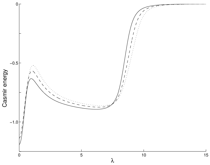
Plots of , and are presented in figure 2. The curves for and have been rescaled vertically, by a factor of and respectively, to make comparison with easier. Note that these three functions are qualitatively very similar. In fact, the Casimir curves and are approximately self-similar up to a factor which diverges as We have opted to use the self-similarity and regularize the diverging factor (the depth of the well at ). So we define the approximate renormalized Casimir energy to be
| (4.39) |
where is the renormalized Casimir energy of the lump. This can be computed exactly using zeta function regularization, because, as we have seen the spectra of the Jacobi operator for the identity map ( lump) and the constant map (the vacuum) are known exactly.
4.3 Zeta function regularization
For the spectrum of the Jacobi operator is known explicitly, namely with multiplicity and with multiplicity for This enables us to calculate the Casimir energy using zeta function regularization. The key idea is to write down the corresponding zeta function
| (4.40) |
leaving out the zero modes. The zeta function (4.40) is absolutely convergent as long as the real part of is sufficiently large. In this region, can be viewed as an analytic function of . We are interested in the Casimir energy which corresponds to the value . In this case, the formal sum in (4.40) is divergent, however, defined as analytic continuation is well-defined. It is convenient to rewrite as the following sum:
| (4.41) |
then we can use formula (5.8) in [9, p. 122] to obtain
The corresponding calculation for the vacuum, whose spectrum is with multiplicity , leads to the zeta function
| (4.42) |
and yields
See also equation (5.34) in [9, p. 126]. Hence, the Casimir energy of the lump on the unit two-sphere can be evaluated using
Hence
This is the energy scale we used to set the renormalized energy scale for our numerically generated Casimir energy function in (4.39).
Our approximation to the Casimir energy is now given by the rescaled and shifted curve in figure 2. It is non-singular and appears to be smooth. It is worth summarizing the approximations involved. Our calculation relies on a conjectured self-similarity of the curves in figure 2. We also assume that we can neglect the effects of crossing modes. In particular, we assume that the zeta-function regularization can be performed pointwise when we regularize the Casimir energy at and Furthermore, we assume that the as because the lumps converge almost everywhere to the vacuum in that limit.
5 The energy spectra
In the following, we describe how to calculate the spectrum of the Laplacian (3.2). In order to make use of the physics literature on this topic we rewrite the Laplacian using angular momentum operators. Note that the operators , , and all satisfy the canonical commutation relations for angular momenta, namely,
and cyclic permutations. Recall that generates the left action, on the target , and generates the right action, on the physical , so we refer to these operators as isospin and spin respectively. Making use of these operators, one sees that the Laplacian (3.2) is
| (5.1) | |||||
Here, we replaced the term using the convenient operator identity
| (5.2) |
We have already shown that commutes with and , as it must, by invariance. In fact, the operators , where is the parity operator, all mutually commute, so we can seek simultaneous eigenstates of these six operators.
5.1 Spin-isospin interchange symmetry
Let and be the eigenvalues of and . It is a somewhat surprising fact that the spectrum of is invariant under interchange of and . Even more surprising is that this remains true even if we give the physical and target spheres different radii. The key to seeing this is the following isometry of any invariant kähler metric on .
Proposition 6
Identify with via . The mapping , induces a mapping . Then is an isometry of any invariant kähler metric on .
Proof.
The identification amounts to thinking of as a vector in the Lie algebra (skew real matrices) and identifying with by left translation. Hence, the map in question is
Let be a curve in with , . Then, with respect to the invariant kähler metric determined by the functions as in Proposition 1,
The image of this curve under is , which has , where
Recalling that the Lie bracket on coincides with minus the vector product on under the natural identification , and the adjoint action of on coincides with the fundamental action on , we find that
Hence is an isometry, as claimed. ∎
Proposition 7
Given and , denote by the simultaneous eigenspace of
with eigenvalues , and , where is any invariant potential. Then and have equal dimension.
Proof.
Under the identification , the left and right actions of on coincide with the natural left and right actions of on . Denote by the induced map on , . Then, since is an isometry and preserves the length of , . Furthermore, interchanges the left and right actions on , so and . Hence, and for all . Now , so , and hence is invertible, so the eigenspaces and are isomorphic. ∎
Note that this interchange symmetry holds for any invariant kähler metric on , so is not special to the case where the domain and target two-spheres have equal radius. Also note that it relies heavily on the kähler property of the metric, and does not follow from invariance alone (or, indeed, just invariance and hermiticity). This is a “hidden” symmetry which one cannot see directly from the field theory. It is an interesting question whether a direct physical argument can be given to explain this symmetry. A construction involving a supersymmetric extension of the model would be a natural candidate.
5.2 Reduction to a Sturm-Liouville problem
The wavefunction is a function . According to the Peter-Weyl theorem [16], the matrix elements of all irreducible unitary representations of the group form an orthonormal basis for . Recall that such representations are labelled by , and that the matrix elements of the representation are functions where . We have chosen the symbol to label the representations because
| (5.3) |
Further, we may choose the basis for so that
| (5.4) |
which is why we have labelled the matrix elements with . For the dependence of we use spherical polar coordinates and expand the angular dependence in spherical harmonics. Hence we may express the wavefunction as follows,
| (5.5) |
where
| (5.6) |
and denote spherical harmonics.
Recall that are mutually commuting, so we may solve the eigenvalue problem for on each simultaneous eigenspace of separately. Clearly, is independent of and so we may, and henceforth will, without loss of generality, set , remembering to multiply all degeneracies by to account for the other values of . Furthermore, by Proposition 7 we may, without loss of generality, assume that , doubling the multiplicity if . Recall that and that and satisfy the angular momentum algebra. Hence a basis for the eigenspace can be constructed, using Clebsch-Gordon coefficients, on which the operators , act naturally
| (5.7) | |||||
| (5.8) | |||||
| (5.9) |
see Appendix B for details.
By expanding the wavefunction as , we may express the Hamiltonian as a matrix of differential operators acting on the vector function , where . Its structure is
| (5.10) |
where are rather complicated but explicitly known functions of (see Proposition 4) and , are matrices corresponding to and respectively. By our choice of basis, is diagonal and has entries with running from (top left) to (bottom right). The matrix corresponding to operator is the only non-diagonal term in the Hamiltonian and is discussed in more detail in appendix B. It mixes states of different , which differ by 2. This leads to a natural chess board structure. Hence, by a reordering of the basis vectors, the operator can be written in block diagonal form with one block corresponding to the states with even and the other block to odd . These blocks correspond to the decompostion of the eigenspace into (even ) and (odd ) parity eigenspaces noting that In summary, for fixed , the eigenvalue problem for any Hamiltonian of the form reduces to a matrix-valued Sturm-Liouville problem on of dimension .
5.3 Boundary conditions
We can now address the eigenvalue equations
| (5.11) |
where is the energy eigenvalue, and the Hamiltonians and are given by (1.3). As just explained, the spectral problem reduces to a sequence of matrix-valued Sturm-Liouville problems indexed by and , where each subproblem has dimension In order to calculate the spectrum of the Hamiltonians and we have to derive not only the relevant differential equations but also the appropriate boundary conditions. For many important examples in mathematical physics, the boundary conditions are determined solely by the requirement that the wavefunction be finite. However, in our case, finiteness is not always sufficient, and we have to apply the theory of singular Sturm-Liouville equations, following [30].
The asymptotic behaviour of the metric on can be obtained by direct calculation:
| (5.12) |
Using the above limits, we obtain the leading order equation for as
| (5.13) |
and the leading order equation for as
| (5.14) |
For equation (5.11) for has a regular singular point. The asymptotic form of the solutions can be derived from (5.14) and is given by11 1 Higher order terms in the expansions for and have been calculated in [24] for with
| (5.15) |
Note that the leading order asymptotic behaviour is independent of the energy eigenvalue . We are interested in solutions that are finite which leads to the condition
| (5.16) |
Using polar coordinates for (3.4) we obtain the two asymptotic behaviours,
for suitable constants and Hence corresponds to the limit-point case, since only the first solution is finite, see e.g. [30] for further details. However, for the situation is slightly more subtle. Both asymptotic solutions are finite. This is known as the limit-circle case.22 2 The same subtlety occurs when solving the Schrödinger equation for the hydrogen atom in spherical polar coordinates. The Hamiltonians lead to the same asymptotic behaviour since the curvature and Casimir energy are finite as .
For it is convenient to analyse the boundary conditions in a different basis so that the operator is diagonal,
where the integer satisfies see appendix B. Then the asymptotic solution follows from (5.13) and is given by
| (5.17) |
for and
| (5.18) |
for Again the leading order behaviour is independent of the energy eigenvalue
Both and contain the scalar curvature function which is known to diverge to infinity as . In fact, using the formula obtained in [37], and accounting for the change in normalizations (recall we are giving the domain and target spheres unit radius), we find the asymptotic formula
| (5.19) |
This adds a term to (5.13), namely,
| (5.20) |
For we can solve (5.20) in terms of modified Bessel functions
| (5.21) |
With the help of asymptotic expansions, see e.g. [1], it can be shown that the leading order is identical to (5.17). For we obtain
| (5.22) |
Since the Casimir energy is bounded, the asymptotic behaviour of as is the same as
As the finite condition (5.16) again leads to two asymptotic behaviours,
for suitable constants and in the case For the curvature term has an influence on the asymptotic behaviour. For we obtain
whereas for and the asymptotic behaviour is
Hence for both solutions lead to finite solutions, resulting in a limit-circle case.
In summary, for all values of and the boundary conditions are either of limit-circle or of limit-point type. Furthermore, both end points are non-oscillatory and independent of the energy eigenvalue This allows us to apply theorem 7.5 in [30] which ensures that the spectrum is purely discrete, bounded below and unbounded above.
If limit-circle endpoints are present, a Sturm-Liouville problem is not self-adjoint unless boundary conditions are imposed. For a non-oscillatory endpoint there is always one solution which is “small”, known as the subdominant solution. More precisely, the subdominant solution unique up to a scalar factor, satisfies
| (5.23) |
where is any linearly independent solution, see theorem 7.15(i) in [30]. In our case, the subdominant solution is the non-singular solution, e.g. as A natural boundary condition is defined by the subdominance condition, i.e. always taking the non-singular solution. Theorem 7.21 in [30] then guarantees that the subdominance condition defines a valid self-adjoint problem known as the Friedrichs extension.
5.4 Numerical results
In the following, we briefly sketch our numerical scheme for with and fixed. The equations for and require minor, but straightforward modifications. We are using a multi-component shooting method which solves a collection of initial value problems (for the eigenvalue equation at fixed ) numerically with a standard adaptive Runge-Kutta method. The first initial value problem has initial values at and the solution of the differential equation (5.11) is evaluated at a matching point . Allowing the initial data to span the dimensional space specified by the boundary condition at , this produces a matrix whose columns consist of above . The second initial value problem has initial values at and is again evaluated at resulting, as the initial data span the boundary condition, in a matrix constructed similarly. By construction, a general solution satisfying the boundary condition at lies, at , in the column span of , while a general solution satisfying the boundary condition at lies, at in the column span of . Hence, is an eigenvalue if these spans have nontrivial intersection, that is, if
| (5.24) |
Having constructed numerically, we find its roots using a bisection method. Typical values of our constants are and
| energy | degeneracy | energy | degeneracy | energy | degeneracy | |||
|---|---|---|---|---|---|---|---|---|
| 0.00 | 1 | 0.22 | 1 | -0.41 | 1 | |||
| 0.13 | 6 | 0.38 | 6 | -0.26∗ | 9 | |||
| 0.18 | 9 | 0.40 | 9 | -0.19∗ | 6 | |||
| 0.29 | 1 | 0.53 | 1 | -0.12 | 1 | |||
| 0.34 | 9 | 0.58 | 9 | -0.01∗ | 9 | |||
| 0.35 | 10 | 0.59∗ | 9 | 0.00∗ | 9 | |||
| 0.38 | 9 | 0.61∗ | 10 | 0.01∗ | 25 | |||
| 0.40 | 30 | 0.63 | 30 | 0.06 | 30 | |||
| 0.49 | 25 | 0.70 | 25 | 0.06∗ | 10 | |||
| 0.54 | 6 | 0.80 | 6 | 0.15 | 6 | |||
| 0.62 | 9 | 0.83 | 9 | 0.22 | 9 | |||
| 0.63 | 30 | 0.87 | 30 | 0.29 | 30 | |||
| 0.64 | 14 | 0.88∗ | 30 | 0.32∗ | 30 | |||
| 0.67 | 30 | 0.91∗ | 14 | 0.33∗ | 25 | |||
| 0.68 | 25 | 0.93 | 25 | 0.34 | 25 | |||
| 0.69 | 42 | 0.95 | 42 | 0.37∗ | 14 | |||
| 0.76 | 25 | 0.96 | 25 | 0.40∗ | 42 | |||
| 0.79 | 70 | 1.01 | 70 | 0.41∗ | 1 | |||
| 0.81 | 1 | 1.07 | 1 | 0.41∗ | 49 | |||
Table 1 shows the lowest energy levels for which corresponds to the Laplacian for the metric, for which also includes the curvature corrections, and for which includes curvature corrections and Casimir energy. Energy levels are rounded to two decimal places. The energy levels are ordered according to their respective energy, and are labelled by isospin quantum number total angular momentum quantum number and parity Curly brackets indicate that the states and have the same energy. States with the same quantum numbers but different energies form sequences of radially excited states. We have chosen to display levels with an energy not greater than the second excited state, which are 19 energy levels in total. The columns “degeneracy” give the number of different states with the same energy. For the degeneracy is given by whereas for it is where the extra factor of arises from the symmetry of the spectrum.
The spectra of and are remarkably similar. The order of the energy levels remains the same apart from two exceptions which are marked with a in table 1 and which will be discussed in more detail later. The Casimir energy leads to significant changes, nevertheless the spectrum still shares some similarities. The ground state of has energy The curvature term increases the energy of the ground state of to whereas the renormalised Casimir energy leads to a decrease in the ground state of to
In order to compare the energies of the excited states, we shift the spectrum of the ground states of and to and then calculate the relative difference of the corresponding energy levels. Hence, the relative difference in energy between the th excited state of and the th excited state of is given by
| (5.25) |
The relative difference of the states of and is and for the first excited states. All the remaining states have a relative difference of less than
As mentioned earlier, some energy levels change order. Therefore, it is useful to calculate the relative error of states with the same quantum numbers The first transposition occurs for the first state and the first state. The relative difference between the energy of the states of and is The second transposition occurs for the first and the first even state, and the states have a relative differences of This leads to the observation that the difference between positive and negative parity states with the same is reduced for compared to . Furthermore, seem to favour states with
As can be seen in table 1 the spectrum of shows many transpositions compared to the spectra of and However, these transpositions occur for states which are close in energy, and the relative positions of the state and the excited states remain almost unchanged. Calculating the relative differences as in formula (5.25) shows that all relative differences are less than
5.5 Changing the radii
It is interesting to consider how our results change if the radii of the domain and target spheres are altered. We adopt the convention that a tilde signifies the case of general while undecorated variables refer to the case . It is immediate from (2.4) that the metric on scales as , and hence, from (3.2), we see that the Laplacian scales as . Now scalar curvature scales in the same way as the Laplacian (as can easily be seen, in this case, from the formula for in [37], for example). Hence, the Hamiltonians and , scale homogeneously, , and so their spectra can be obtained from table 1 by a simple rescaling. Now the energies shown in this table are quantum corrections to the classical energy, which, by the Lichnerowicz bound is . Hence, for , , the total energy of the th energy level is
| (5.26) |
where is the eigenvalue of . It is interesting to note that the quantum correction becomes (naively) dominant in the case of small target space ( small).
The behaviour of is more subtle because the Casmir energy scales differently from the other terms. To see this, we determine how the Jacobi operator for a harmonic map scales under homotheties of and .
Proposition 8
Let be harmonic with Jacobi operator . If , , where are constants, then the Jacobi operator of as a harmonic map is
Proof.
Let be a smooth two-parameter variation of , with , . We have, in obvious notation,
∎
Since is (formally) a sum of square roots of eigenvalues of , we see that it scales as . Hence, the scaling behaviour of is inhomogeneous, and, except in the special case that , the spectrum of cannot be deduced directly from the spectrum of . Since is independent of the radius whereas the spectra of and scale like the effect of the Casimir energy becomes less important for small We have also numerically checked that a smaller radius of the target sphere reduces the effect of the Casimir energy term significantly. For example for and there is only one transposition, compared to the spectrum.
Throughout this paper we have used the convention that If we reinstate the parameter then the classical energy scales like the Casimir energy scales like whereas the Laplacian and curvature terms scale like Hence, can be removed by redefining so the semi-classical limit coincides (formally) with the planar limit

5.6 Deformation to the Fubini-Study metric
As a nontrivial test of our calculations we calculate how the spectrum changes as the metric is smoothly deformed from the metric to the well-known Fubini-Study metric of where the spectrum and degeneracy of the Laplace operator have been calculated explicitly. We consider the one-parameter family of invariant kähler metrics defined, as in Proposition 1, by the functions
| (5.27) |
where and are given in (2.14) and (2.12), respectively, and the factor of ensures that the eigenvalues of the two Laplacians are of the same order of magnitude. The th eigenvalue of the Laplacian for the Fubini-Study metric on with constant holomorphic sectional curvature (and hence coefficient function ) is
| (5.28) |
with degeneracy
| (5.29) |
for [6]. Although it is not made clear in [6], the degeneracy of must be by the Hodge isomorphism theorem, since is connected, hence which equals the dimension of the space of harmonic -forms. Note that for is an integer divisible by In figure 3 we show how the energy levels change as the parameter in (5.27) is increased from (the metric) to (the Fubini-Study metric). We distinguish between states with even and odd parity. The ground state is for both metrics. In figure 3 we follow all the energy levels of table 1, and it can be seen how the different energy levels become degenerate at the Fubini-Study limit. Our numerically computed energy levels agree with the exact result to at least two decimal places, when we take into account the factor in and normalize the Fubini-Study energy by a factor of which arises from the factor in (5.27).
Our numerical scheme at does not find all eigenfunctions of on , because, except for the ground state, we impose a boundary condition which forces the wavefunction to vanish on , the boundary of at infinity. It is known [37] that coincides with the image of the inclusion , . The stabilizer of this subset of in , the isometry group of , is isomorphic to (the isometry group of itself). So, given an eigenfunction vanishing on , the action generates a -dimensional orbit of degenerate eigenfunctions which do not vanish on (because and ). Hence, we expect the degeneracies found by our numerics (at ) to be a factor smaller than the degeneracies of the true Laplacian on . This is precisely what we find. For example, the degeneracy of the second eigenvalue is which corresponds to the levels and with degeneracy see table 1. Similarly, corresponds to and with Further, which corresponds to and whose degeneracies add up to as expected. To display all the levels which contribute to the fourth energy eigenvalue of we have also included the level in figure 3. Note that the second excited state contributes to the fifth energy eigenvalue of
6 Concluding remarks
In this paper we discussed the semi-classical quantization of soliton dynamics for lumps moving on a 2-sphere. We followed Moss and Shiiki [28] who derived a Born-Oppenheimer approximation to the quantum dynamics based on the moduli space approximation. We were able to evaluate three different truncations of the Born-Oppenheimer Hamiltonian namely the geometric Laplacian the first geometric correction given by the scalar curvature of the moduli space, and the Hamiltonian which consists of together with the Casimir energy. The Casimir energy is notoriously difficult to evaluate. At and the spectrum of the Jacobi operator is known explicitly. Our approach is to calculate the regularized Casimir energy using zeta-function regularization for and Then the intermediate values are calculated using an approximate self-similarity of the eigenvalue spectrum. We calculated the first energy levels for and and found that the first two spectra are remarkably similar whereas the inclusion of the Casimir energy leads to significant changes. There is an overall shift of the spectrum of and The relative errors between and are for the first excited state and less that for other excited states. By contrast, the relative errors between and are as high as for some excited states. There are only two transpositions of states where energy levels of do not have the same order compared to the spectrum. However, the spectrum of shows many transpositions.
We proved that all the spectra enjoy a rather surprising spin-isospin exchange symmetry. The proof rested on the identification of a hidden isometry of which becomes manifest only after one identifies . As a non-trivial check of our calculations we calculated how the energy levels change when we interpolate between the metric and the Fubini-Study metric on We reproduced the known spectrum for and discussed the degeneracies of the energy levels.
Our approach allows us to calculate the spectrum of the Laplacian for any invariant kähler metric on . One interesting choice is for which the coefficient of vanishes in (5.1). In this case, the angular momentum operator also commutes with the Hamiltonian and becomes an additional quantum number.
The lump dynamics serves as a toy model for other solitons. For example in three spatial dimensions, two physically relevant models are the Skyrme model [34] and the Faddeev-Hopf model [10, 11]. In both models, the solitons can be quantized as fermions due to so-called Finkelstein-Rubinstein constraints [12]. Adkins, Nappi and Witten first quantized the Skyrmion in [2] where is the topological charge. The effects of the Casimir energy on the predictions of the Skyrme model in the sector have been discussed in great detail in [26]. The authors calculated the 1-loop corrections to various physical quantities using phase-shift techniques to evaluate the Casimir energy. For higher topological charge the ground and lowest excited states in the Skyrme model and the Faddeev-Hopf model were calculated in [15, 18, 4] and [19] using zero-mode quantization and Finkelstein-Rubinstein constraints. The results of this paper suggest that the order of the states would remain the same, with minor changes, if the curvature correction in the Born-Oppenheimer approximation was taken into account. However, the Casimir energy could lead to significant changes in the order of states. A more careful analysis of higher order terms in these models, and in particular, of the Casimir energy, would be very useful.
Acknowledgments
SK is grateful to NS Manton for interesting discussions at various stages of the project. The authors would like to thank James McGlade and Lamia Al Qahtani for useful discussions. McGlade derived the spectrum for zero isospin in his thesis [24].
Appendix
Appendix A The rough Laplacian
In this appendix we will compute in detail the action of the rough Laplacian on sections of of the form
| (A.1) |
Recall that the unit sphere, are the usual polar coordinates on or , , is an orthonormal frame on or , , , and is a map of the form in polar coordinates. Now, given a map between Riemannian manifolds , the pullback connexion is the unique connexion on the vector bundle satisfying the axioms
| (A.2) | |||||
| (A.3) | |||||
| (A.4) |
for all , , and , where is the Levi-Civita connexion on . In our case (which coincides with ) is determined by its action on the frame ,
| (A.5) |
where is the coframe dual to . From this we may deduce how acts on . By property (A.4) and (A.5),
| (A.6) | |||||
| (A.7) | |||||
| (A.8) | |||||
| (A.9) |
The rough Laplacian has 4 terms,
| (A.10) |
We evaluate these in turn, for . First
| (A.11) |
The second term is more involved:
| (A.12) | |||||
| (A.13) | |||||
The third term vanishes since , while the fourth term is
| (A.14) |
Assembling the pieces, one sees that
| (A.15) | |||||
as claimed in equation (4.14).
Appendix B Angular momentum calculations
In this appendix we briefly describe the evaluation of the operator We closely follow the notation in [8]. Note the spin quantum number satisfies since . We choose the following convention for the spherical harmonics,
| (B.1) |
where the associated Legendre polynomials are given by
| (B.2) |
Note that and
| (B.3) |
It is easy to show that and we showed in section 3 that this operator commutes with and see equation (3.8) where and Hence, the operator does not change the quantum numbers and Furthermore, the matrix elements are independent of and hence we can choose without loss of generality and . We need to evaluate
| (B.4) |
which is a by matrix, because the angular momentum quantum numbers satisfy . Since is a Hermitian operator the matrix is Hermitian, namely
| (B.5) |
Using Clebsch-Gordan coefficients (B.4) can be rewritten as
| (B.6) |
The operator can be written in terms of spherical harmonics as
| (B.7) |
Hence, we only need to evaluate
| (B.8) | |||||
| (B.9) | |||||
| (B.10) |
and
| (B.11) |
which can be calculated using (4.6.3) in [8], namely,
| (B.12) | |||
where the two matrices in (B) correspond to symbols. The symbol
| (B.18) |
vanishes unless which can be used to show that vanishes in the cases or . For example, for the only allowed values of the angular momentum are and which vanishes since
Following the notation in [8], the Clebsch-Gordan coefficients and the symbols have real entries. Hence, is a real matrix and (B.5) implies that is symmetric. Note that the eigenvalues of are which can be explained as follows. Heuristically, is the projection of the total angular momentum operator onto the direction. Hence, it can be rotated by a change of variables to which has eigenvalues The highest possible value of is because the dimension of is
Now, we can evaluate the matrix (B.4) for various values of and using Maple, for example. For small values the formulae are more tractable. For example for we obtain
| (B.19) |
We showed in section 5.1 that there is a symmetry for the respective matrices This was verified by explicit calculation for all values in table 1. As can be seen in (B.19) there is a natural chess board structure in the matrix which follows from the fact that vanishes unless and hence vanishes unless or
References
- [1] M. Abramowitz and I. A. Stegun, Handbook of Mathematical Functions (Dover Publications, tenth edition, 1972).
- [2] G. S. Adkins, C. R. Nappi and E. Witten, “Static Properties of Nucleons in the Skyrme Model,” Nucl. Phys. B 228 (1983) 552-584.
- [3] J.M. Baptista, “Some special Kähler metrics on and their holomorphic quantization” J. Geom. Phys. 50 (2004) 1-27.
- [4] R. A. Battye, N. S. Manton, P. M. Sutcliffe and S. W. Wood, “Light Nuclei of Even Mass Number in the Skyrme Model,” Phys. Rev. C 80 (2009) 034323-034338.
- [5] A.L. Besse, Einstein Manifolds (Springer-Verlag, Berlin, Germany, 2002).
- [6] M. Berger, P. Gauduchon, E. Mazet, Le Spectre d’une Variété Riemannienne (Springer-Verlag, 1971).
- [7] P. Bizon, T. Chmaj and Z. Tabor, “Formation of singularities for equivariant -dimensional wave maps into the 2-sphere” Nonlinearity 14 (2001) 1041-53.
- [8] E.R. Edmonds, Angular Momentum in Quantum Mechanics (Princeton University Press, Princeton, New Jersey, 1960).
- [9] E. Elizalde, S.D. Odintsov, A. Romeo, A.A. Bytsenko and S. Zerbini, Zeta Regularization Techniques with Applications (World Scientifique, Singapore, 1994).
- [10] L. D. Faddeev, “Quantisation of solitons” (Preprint IAS Print-75-QS70, Princeton, 1975).
- [11] L. D. Faddeev and A. J. Niemi, “Knots and particles” Nature 387 (1997) 58-61.
- [12] D. Finkelstein and J. Rubinstein, “Connection between spin, statistics, and kinks” J. Math. Phys. 9 (1968) 1762-1779.
- [13] G.W. Gibbons and N.S. Manton, “Classical and quantum dynamics of BPS monopoles” Nucl. Phys. B274 (1986) 183-224.
- [14] M. Haskins and J.M. Speight, “The geodesic approximation for lump dynamics and coercivity of the Hessian for harmonic maps” J. Math. Phys. 44 (2003) 3470-94.
- [15] P. Irwin, “Zero mode quantization of multi - Skyrmions,” Phys. Rev. D 61 (2000) 114024-114057.
- [16] A.W. Knapp, Representation Theory of Semisimple Groups, (Princeton University Press, Princeton NJ, USA, 1986), p17.
- [17] S. Kobayashi and K. Nomizu, Foundations of Differential Geometry (John Wiley, New York, USA, 1996) Volume II, p167.
- [18] S. Krusch, “Homotopy of rational maps and the quantization of skyrmions” Annals Phys. 304 (2003) 103-127.
- [19] S. Krusch and J.M. Speight, “Fermionic quantization of Hopf solitons” Commun. Math. Phys. 264 (2006) 391-410.
- [20] A. Lichnerowicz, “Applications harmoniques et variétés kähleriennes” Symp. Math. Bologna 3 (1970) 341-402.
- [21] J.M. Linhart and L.A. Sadun, “Fast and slow blowup in the model and the -dimensional Yang-Mills model” Nonlinearity 15 (2002) 219-238.
- [22] N.S. Manton, “A remark on the scattering of BPS monopoles” Phys. Lett. 110B (1982) 54-56.
- [23] N.S. Manton and P.M. Sutcliffe, Topological Solitons (Cambridge University Press, Cambridge, UK, 2004).
- [24] J.A. McGlade, The Dynamics of Topological Solitons within the Geodesic Approximation (PhD Thesis, University of Leeds, 2005).
- [25] J.A. McGlade and J.M. Speight, “Slow equivariant lump dynamics on the two-sphere” Nonlinearity 19 (2006) 441-452.
- [26] F. Meier and H. Walliser, “Quantum Corrections to Baryon Properties in Chiral Soliton Models,” Phys. Rept. 289 (1997) 383-448.
- [27] I.G. Moss, “Soliton vacuum energies and the CP(1) model” Phys. Lett. B460 (1999) 103-106.
- [28] I.G. Moss and N. Shiiki, “Quantum mechanics on moduli spaces” Nucl. Phys. B565 (2000) 345-362.
- [29] I. G. Moss, N. Shiiki and T. Torii, “Vacuum energy of CP(1) solitons,” (Preprint: arXiv:hep-ph/0103240, 2001).
- [30] J.D. Pryce, Numerical Solution of Sturm-Liouville Problems (Oxford University Press, Oxford, UK, 1993).
- [31] I. Rodnianski and J. Sterbenz, “On the Formation of Singularities in the Critical Sigma-Model” Ann. Math. 172 (2010) 187-242.
- [32] P.J. Ruback, “Sigma model solitons and their moduli space metrics” Commun. Math. Phys. 116 645-58.
- [33] L. Sadun and J.M. Speight, “Geodesic incompleteness in the model on a compact Riemann surface” Lett. Math. Phys. 43 (1998) 329-34.
- [34] T. H. R. Skyrme, “A nonlinear field theory” Proc. Roy. Soc. Lond. A260 (1961) 127-138.
- [35] R.T. Smith, “The second variation formula for harmonic mappings” Proc. Amer. Math. Soc. 47 (1975) 229-36.
- [36] J.M. Speight, “Low energy dynamics of a lump on the sphere” J. Math. Phys. 36 (1995) 796-813.
- [37] J.M. Speight, “The geometry of spaces of harmonic maps and ” J. Geom. Phys. 47 (2003) 343-368.
- [38] D. Stuart, “Dynamics of abelian Higgs vortices in the near Bogomolny regime” Commun. Math. Phys. 159 (1994) 51-91.
- [39] D. Stuart, “The geodesic approximation for the Yang-Mills-Higgs equations” Commun. Math. Phys. 166 (1994) 149-90.
- [40] H. Urakawa, Calculus of Variations and Harmonic Maps (American Mathematical Society, Providence RI, USA, 1993).
- [41] T.J. Willmore, Riemannian Geometry (Clarendon Press, Oxford, UK, 1993) p57.