Channel Capacity under
Sub-Nyquist Nonuniform Sampling

Yuxin Chen Andrea J. Goldsmith Yonina C. Eldar ^†^†thanks: Y. Chen is with the Department of Electrical Engineering, Stanford University, Stanford, CA 94305, USA (e-mail: yxchen@stanford.edu). A. J. Goldsmith is with the Department of Electrical Engineering, Stanford University, Stanford, CA 94305, USA (e-mail: andrea@ee.stanford.edu). Y. C. Eldar is with the Department of Electrical Engineering, Technion, Israel Institute of Technology Haifa, Israel 32000 (e-mail: yonina@ee.technion.ac.il). This work was supported in part by the NSF Center for Science of Information, the Interconnect Focus Center of the Semiconductor Research Corporation, and BSF Transformative Science Grant 2010505. This paper was presented in part at the 2012 IEEE International Symposium on Information Theory [1]. Copyright (c) 2012 IEEE. Personal use of this material is permitted. However, permission to use this material for any other purposes must be obtained from the IEEE by sending a request to pubs-permissions@ieee.org.

Abstract

This paper investigates the effect of sub-Nyquist sampling upon the capacity of an analog channel. The channel is assumed to be a linear time-invariant Gaussian channel, where perfect channel knowledge is available at both the transmitter and the receiver. We consider a general class of right-invertible time-preserving sampling methods which include irregular nonuniform sampling, and characterize in closed form the channel capacity achievable by this class of sampling methods, under a sampling rate and power constraint. Our results indicate that the optimal sampling structures extract out the set of frequencies that exhibits the highest signal-to-noise ratio among all spectral sets of measure equal to the sampling rate. This can be attained through filterbank sampling with uniform sampling at each branch with possibly different rates, or through a single branch of modulation and filtering followed by uniform sampling. These results reveal that for a large class of channels, employing irregular nonuniform sampling sets, while typically complicated to realize, does not provide capacity gain over uniform sampling sets with appropriate preprocessing. Our findings demonstrate that aliasing or scrambling of spectral components does not provide capacity gain, which is in contrast to the benefits obtained from random mixing in spectrum-blind compressive sampling schemes.

Index Terms:

nonuniform sampling, irregular sampling, sampled analog channels, sub-Nyquist sampling, channel capacity, Beurling density, time-preserving sampling systems

I Introduction

The capacity of analog Gaussian channels and their capacity-achieving transmission strategies were pioneered by Shannon [2], which has provided fundamental insights for modern communication system design. Shannon’s work focused on capacity of analog channels sampled at or above twice the channel bandwidth. However, these results do not explicitly account for sub-Nyquist sampling rate constraints that may be imposed by hardware limitations. This motivates exploration of the effects of sub-Nyquist sampling upon the capacity of an analog Gaussian channel, and the fundamental capacity limits that result when considering general sampling methods that include irregular nonuniform sampling.

I-A Related Work and Motivation

Shannon introduced and derived the information theoretic metric of channel capacity for time-invariant analog waveform channels[2], which established the optimality of water-filling power allocation based on signal-to-noise ratio (SNR) over the spectral domain [3, 4]. A key idea in determining the analog channel capacity is to convert the continuous-time channel into a set of parallel discrete-time channels based on the Shannon-Nyquist sampling theorem [5]. This paradigm was employed, for example, by Medard et. al. to bound the maximum mutual information in time-varying channels [6, 7], and was used by Forney et. al. to investigate coding and modulation for Gaussian channels [8]. Most of these results focus on the analog channel capacity commensurate with uniform sampling at or above the Nyquist rate associated with the channel bandwidth. There is another line of work that characterizes the effects upon information rates of oversampling with quantization [9, 10]. In practice, however, hardware and power limitations may preclude sampling at the Nyquist rate for a wideband communication system.

More general irregular sampling methods beyond pointwise uniform sampling have been extensively studied in the sampling literature, e.g. [11, 12, 13]. One example is sampling on non-periodic quasi-crystal sets, which has been shown to be stable for bandlimited signals [14, 15]. These sampling approaches are of interest in some realistic situations where signals are only sampled at a nonuniformly spaced sampling set due to constraints imposed by data acquisition devices. Many sophisticated reconstruction algorithms have been developed for the class of bandlimited signals or, more generally, the class of shift-invariant signals [16, 17, 11]. For all these nonuniform sampling methods, the Nyquist sampling rate is necessary for perfect recovery of bandlimited signals [18, 19, 11].

However, for signals with certain structure, the Nyquist sampling rate may exceed that required for perfect signal reconstruction from the samples [20, 21]. For example, consider multiband signals, whose spectral contents reside within several subbands over a wide spectrum. If the spectral support is known, then the necessary sampling rate for the multiband signals is their spectral occupancy, termed the Landau rate [22]. Such signals admit perfect recovery when sampled at rates approaching the Landau rate, provided that the sampling sets are appropriately chosen (e.g. [23, 24]). One type of sampling mechanism that can reconstruct multiband signals sampled at the Landau rate is a filter bank followed by sampling, studied in [25, 26, 27]. Inspired by recent “compressive sensing” [28, 29, 30] ideas, spectrum-blind sub-Nyquist sampling for multiband signals with random modulation has been developed [31] as well.

Although sub-Nyquist nonuniform sampling methods have been extensively explored in the sampling literature, they are typically investigated either under a noiseless setting, or based on statistical reconstruction measures (e.g. mean squared error (MSE)) instead of information theoretic measures. Gastpar et al [32] studied the necessary sampling density for nonuniform sampling. Recent work by Wu and Verdu [33] investigated the tradeoff between the number of samples and the reconstruction fidelity through information theoretic measures. However, these works did not explicitly consider the capacity metric for an analog channel. The most relevant capacity result to our work was by Berger et al [34], who related MSE-based optimal sampling with capacity for several special types of channels. But they did not derive the sub-Nyquist sampled channel capacity for more general channels, nor did they consider nonuniformly spaced sampling. Our recent work [35] established a new framework that characterizes sampled capacity for a broad class of sampling methods, including filter and modulation bank sampling [36, 31, 37]. For these sampling methods, we determined optimal sampling structures based on capacity as a metric, illuminated intriguing connections between MIMO channel capacity and capacity of undersampled channels, as well as a new connection between capacity and MSE. However, this prior work did not investigate analog channel capacity using more general nonuniform sampling under a sub-Nyquist sampling rate constraint.

One interesting fact discovered in [35] is the non-monotonicity of capacity with sampling rate under filter- and modulation-bank sampling, assuming an equal sampling rate per branch for a given number of branches. This indicates that more sophisticated sampling techniques, adaptive to the channel response and the sampling rate, are needed to maximize capacity under sub-Nyquist rate constraints, including both uniform and nonuniform sampling. However, none of the aforementioned work has investigated the question as to which sampling method can best exploit channel structure, thereby maximizing sampled capacity under a given sampling rate constraint. Although several classes of sampling methods were shown in [35] to have closed-form capacity solutions, the capacity limits might not even exist for general sampling methods. This raises the question as to whether there exists a capacity upper bound over a general class of sub-Nyquist sampling systems beyond the classes we discussed in [35] and, if so, when the bound is achievable. That is the question we investigate herein.

I-B Contributions and Organization

Our main contribution is to derive the capacity of sub-Nyquist sampled analog channels for a general class of right-invertible time-preserving nonuniform sampling methods, under a sub-Nyquist sampling rate constraint. The channel is assumed to be a linear time-invariant (LTI) Gaussian channel, where perfect channel knowledge is available at both the transmitter and the receiver. The class of sampling systems we consider subsumes sampling structures employing irregular nonuniform sampling grids.

We first develop in Theorem 2 an upper bound on the sampled channel capacity, which corresponds to the capacity of a channel whose spectral occupancy is no larger than the sampling rate $f_{s}$ . As a key step in the analysis framework for Theorem 2, we characterize in closed form the sampled channel capacity for any specific periodic sampling system, formally defined in Definition 8 (Lemma 1). We demonstrate that this fundamental capacity limit can be achieved by filterbank sampling with varied sampling rates at different branches, or by a single branch of modulation and filtering followed by a uniform sampling set (Theorems 3-4). In particular, the optimal sampler extracts out a spectral set of size $f_{s}$ with the highest SNR, and suppresses all signal and noise components outside this spectral set.

Our results indicate that irregular nonuniform sampling sets, while typically complicated to realize in hardware, do not increase channel capacity relative to analog preprocessing with regular uniform sampling sets. We also show that when optimal filterbank or modulation sampling is employed, a mild perturbation of the optimal sampling grid does not change the capacity. Our findings demonstrate that aliasing or scrambling of spectral contents does not provide capacity gain. This is in contrast to the benefits obtained from random mixing of frequency components in many sub-Nyquist sampling schemes with unknown signal support (e.g. [31]).

The main innovation of this paper compared to our previous sub-sampled channel capacity results in [35] is as follows.

•

While [35] characterizes the capacity under two types of sampling mechanisms that are widely used in practice (filter-bank sampling and modulation-bank sampling), the focus of this paper is instead to develop capacity results over a much more general class of sampling methods.
•

While all results of [35] hold only under uniform sampling, our analysis herein accommodates irregular nonuniform sampling. Our results in turn corroborate the optimality of uniform sampling in achieving sampled capacity, assuming that the analog channel output is appropriately pre-processed.

The remainder of the paper is organized as follows. In Section II, we introduce our system model of sampled analog channels, and provide formal definitions of time-preserving systems, sampling rates, and sampled channel capacity. We then develop, in Section III-A, an upper bound on the sampled channel capacity ranging over all right-invertible time-preserving sampling methods, along with an approximate analysis highlighting insights into the result. The achievability of this upper bound is derived in Section III-B. The proof of Theorem 2 is provided in Appendix A. The implications of our main results are summarized in Section IV.

Before continuing, we introduce some notation that will be used throughout. We use $\mu\left(\cdot\right)$ to represent the Lebesgue measure, and denote by $\mathcal{F}$ and $\mathcal{F}^{-1}$ the Fourier and inverse Fourier transform, respectively. We let $[x]^{+}\overset{\Delta}{=}\max\left(x,0\right)$ , and use $\mathrm{card}\left(A\right)$ to denote the cardinality of a set $A$ . These and other notation in the paper are summarized in Table I.

Table I: Summary of Notations and Parameters

$\mu(\cdot)$	Lebesgue measure
$\Lambda$	sampling set $\left\{t_{n}:n\in Z\right\}$
$D^{+}(\Lambda),$ $D^{-}(\Lambda)$ , $D(\Lambda)$	upper, lower and uniform Beurling densities of $\Lambda$
$\mathcal{L}_{2}\left(\Omega\right)$	set of measurable functions $f$ supported on the set $\Omega$ such that $\int\left\|f\right\|^{2}\mathrm{d}\mu<\infty$
$\mathbb{S}_{+}$	set of positive semidefinite matrices
$h(t)$ , $H(f)$	impulse response and frequency response of the LTI analog channel
$s_{i}(t)$ , $S_{i}(f)$	impulse response and frequency response of the $i$ th (post-modulation) filter
$p(t)$ , $P(f)$	impulse response and frequency response of the pre-modulation filter
$\mathcal{S}_{\eta}(f),s_{\eta}(t)$	power spectral density of the noise $\eta(t)$ and $s_{\eta}\left(t\right):=\mathcal{F}^{-1}\left(\sqrt{\mathcal{S}_{\eta}\left(f\right)}\right)$
$f_{s}$ , $T_{s}$	aggregate sampling rate and the corresponding sampling interval ( $T_{s}=1/f_{s}$ )
$q(t,\tau)$	impulse response of the sampling system, i.e. the output seen at time $t$ due to an impulse in the input at time $\tau$ .
$T_{q},f_{q}$	period of the modulating sequence $q(t)$ such that $T_{q}=1/f_{q}$
$\mathcal{F}$ , $\mathcal{F}^{-1}$	Fourier transform and inverse Fourier transform

II Sampled Channel Capacity

II-A System Model

We consider an analog waveform channel, which is modeled as an LTI filter with impulse response $h(t)$ and frequency response $H(f)=\int_{-\infty}^{\infty}h(t)\exp(-j2\pi ft)\text{d}t$ . With $x(t)$ denoting the transmitted signal, the analog channel output is given by

r(t)=h(t)*x(t)+\eta(t),

(1)

where the noise process $\eta(t)$ is assumed to be an additive stationary zero-mean Gaussian process with power spectral density $\mathcal{S}_{\eta}\left(f\right)$ . We also define $s_{\eta}\left(t\right):=\mathcal{F}^{-1}\left(\sqrt{\mathcal{S}_{\eta}\left(f\right)}\right)$ . Unless otherwise specified, we assume throughout that perfect channel state information (i.e. the knowledge of both $H(f)$ and $\mathcal{S}_{\eta}(f)$ ) is available at both the transmitter and the receiver.

The analog channel output $r(t)$ is passed through $M$ ( $1\leq M\leq\infty$ ) branches of linear preprocessing systems, each followed by a pointwise sampler, as illustrated in Fig. 1. The preprocessed output $y_{i}(t)$ at the $i$ th branch is obtained by applying a linear bounded operator $\mathcal{T}_{i}$ to the channel output $r(t)$ :

\displaystyle y_{i}(t)

\displaystyle=\mathcal{T}_{i}\left(r(t)\right)=\int q_{i}\left(t,\tau\right)r\left(\tau\right)\mathrm{d}\tau,

(2)

where $q_{i}(t,\tau)$ denotes the impulse response of the time-varying system represented by $\mathcal{T}_{i}$ , i.e. the output seen at time $t$ due to an impulse in the input at time $\tau$ . Note that the linear operator $\mathcal{T}_{i}$ can be time-varying, which subsumes filtering and modulation as special cases. For example, a modulation system $\mathcal{T}_{i}\left(x(t)\right)=p(t)x(t)$ for some given modulation sequence $p(t)$ has an impulse response $q(t,\tau)=p(\tau)\delta\left(t-\tau\right)$ . A cascade combination of two systems $\mathcal{T}_{1}$ and $\mathcal{T}_{2}$ has an impulse response $q(t,\tau)=\int_{-\infty}^{\infty}q_{2}(t,\tau_{1})q_{1}(\tau_{1},\tau)\mathrm{d}\tau_{1}$ , with $q_{1}\left(\cdot,\cdot\right)$ and $q_{2}(\cdot,\cdot)$ denoting respectively the impulse responses of $\mathcal{T}_{1}$ and $\mathcal{T}_{2}$ [38]. When an operator $\mathcal{T}$ is LTI, we use $q(\tau):=q(t,t-\tau)$ as shorthand to represent its impulse response.

The pointwise sampler following the preprocessor can be uniform or irregular [11]. Specifically, the preprocessed output $y_{i}(t)$ (at the $i$ th branch) is sampled at times $t_{i,n}\left(n\in\mathbb{Z}\right)$ , yielding a sample sequence $y_{i}[n]=y_{i}\left(t_{i,n}\right)$ . Here, we define the sampling set $\Lambda_{i}$ at the $i$ th branch as

\Lambda_{i}:=\left\{t_{i,n}\mid n\in\mathbb{Z}\right\}.

(3)

In particular, if $t_{i,n}=nT_{i,s}$ , then the sampling set at the $i$ th branch is said to be uniform with period $T_{i,s}$ .

Refer to caption — Figure 1: The input $x(t)$ is passed through the analog channel and contaminated by noise $\eta(t)$ . The analog channel output $r(t)$ is then passed through $M\text{ }(1\leq M\leq\infty)$ linear preprocessing system $\left\{\mathcal{T}_{i}\mid 1\leq i\leq M\right\}$ . At the $i$ th branch, the preprocessed output $y_{i}(t)$ is sampled on the sampling set $\Lambda_{i}=\left\{t_{i,n}\mid n\in\mathbb{Z}\right\}$ .

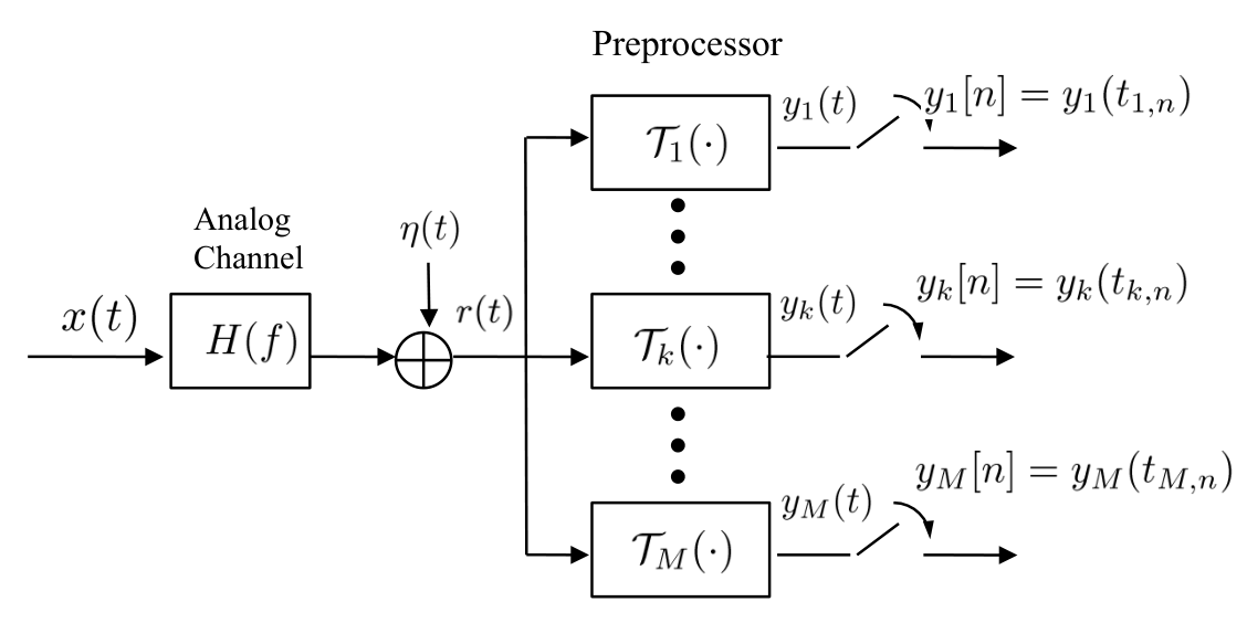
II-B Sampling Rate Definition

Our metric of interest is the sampled channel capacity under a sampling rate constraint. We first formally define sampling rate for general nonuniform sampling mechanisms.

In general, the sampling set $\Lambda=\left\{t_{n}\mid n\in\mathbb{Z}\right\}$ may be irregular and hence aperiodic, which calls for a generalized definition of sampling rate. One notion commonly used in sampling theory is the Beurling density introduced by Beurling [18] and Landau [22], as defined below [11].

Definition 1 (Beurling Density).

For a sampling set $\Lambda=\left\{t_{k}\mid k\in\mathbb{Z}\right\}$ , the upper and lower Beurling density are given respectively as

	$\displaystyle D^{+}\left(\Lambda\right)$	$\displaystyle=\lim_{r\rightarrow\infty}\sup_{z\in\mathbb{R}}\frac{\text{card}\left(\Lambda\cap\left[z,z+r\right]\right)}{r},$
	$\displaystyle D^{-}\left(\Lambda\right)$	$\displaystyle=\lim_{r\rightarrow\infty}\inf_{z\in\mathbb{R}}\frac{\text{card}\left(\Lambda\cap\left[z,z+r\right]\right)}{r}.$

When $D^{+}\left(\Lambda\right)=D^{-}\left(\Lambda\right)$ , the sampling set $\Lambda$ is said to be of uniform Beurling density $D\left(\Lambda\right):=D^{-}\left(\Lambda\right)$ .

When the sampling set is uniform with period $T_{s}$ , the Beurling density is $D(\Lambda)=1/T_{s}$ , which coincides with the conventional definition of sampling rate. The notion of Beurling density allows the Shannon-Nyquist sampling theorem to be extended to nonuniform sampling. Moreover, we will use Beurling density to define sampling rate for a large class of sampling mechanisms with preprocessing.

Under a nonuniform sampling set $\Lambda$ , the set of exponential functions $\left\{\exp\left(j2\pi t_{n}f\right)\mid n\in\mathbb{Z}\right\}$ forms a non-harmonic Fourier series [12]. Whether the class of original signals are recoverable from the nonuniform sampled sequence is determined by the completeness of the associated non-harmonic set. In particular, when $\Lambda$ is uniform, the set $\left\{\exp\left(j2\pi t_{n}f\right)\mid n\in\mathbb{Z},t_{n}=n/f_{s}\right\}$ with $D(\Lambda)=f_{s}$ forms a Riesz basis [39] of $\mathcal{L}_{2}(-f_{s}/2,f_{s}/2)$ by the Shannon-Nyquist sampling theorem. For the class of sampling systems without preprocessing, a fundamental rate limit necessary for perfect reconstruction of bandlimited signals has been characterized by Landau using the definition of Beurling density, as stated in the following theorem.

Theorem 1 (Landau Rate [22]).

Consider the set $\mathcal{B}_{\Omega}$ of all signals whose spectral contents are supported on the frequency set $\Omega$ . Suppose that pointwise sampling without preprocessing is employed with a sampling set $\Lambda$ . If all signals $f(t)\in\mathcal{B}_{\Omega}$ can be uniquely determined by the samples $\left\{f(t_{n})\mid t_{n}\in\Lambda\right\}$ , then one must have $D^{-}(\Lambda)\geq\mu\left(\Omega\right)$ . The value $\mu\left(\Omega\right)$ is termed the Landau rate.

Theorem 1 characterizes the fundamental sampling rate requirement for perfect signal reconstruction under pointwise sampling without preprocessing. In particular, when $\Omega=[-B/2,B/2]$ , Theorem 1 reduces to the Shannon-Nyquist theorem.

We will thereby use Beurling density to characterize the sampling rate for a general sampling set. However, since the preprocessor might distort the time scale of the input, the resulting “sampling rate” might not characterize the true sampling rate applied to the original signal, as illustrated in the following example.

Example 1 (Compressor).

Consider a preprocessing system defined by the relation

y(t)=\mathcal{T}\left(r(t)\right)=r\left(Lt\right)

with $L\geq 2$ being a positive integer. If we apply a uniform sampling set $\Lambda=\{t_{n}:t_{n}=n/f_{s}\}$ on the preprocessed output $y(t)$ , the sampled sequence at a “sampling rate” $f_{s}$ is given by

y[n]=y\left(n/f_{s}\right)=r\left(nL/f_{s}\right),

which corresponds to sampling the system input $r(t)$ at rate $f_{s}/L$ . The compressor effectively time-warps the signal, thus resulting in a mismatch of the time scales between the input and output.

The compressor example illustrates that the notion of sampling rate may be misleading for systems that experience time warping. Hence, this paper will focus only on sampling that preserves time scales. One class of linear systems that preserves time scales are modulation operators $\left(y(t)=p(t)x(t)\right)$ , which perform pointwise scaling of the input, and hence do not change the time scale. Another class is the periodic system which includes LTI filtering, defined as follows.

Definition 2 (Periodic System).

A linear preprocessing system is said to be periodic with period $T_{q}$ if its impulse response $q(t,\tau)$ satisfies

q(t,\tau)=q(t+T_{q},\tau+T_{q}),\quad\forall t,\tau\in\mathbb{R}.

(4)

A more general class of systems that preserve the time scale can be generated through modulation and periodic subsystems. Specifically, we can define a general time-preserving system by connecting a set of modulation or periodic operators in parallel or in serial. This leads to the following definition.

Definition 3 (Time-preserving System).

Given an index set $\mathcal{I}$ , a preprocessing system $\mathcal{T}:x(t)\mapsto\left\{y_{k}(t),k\in\mathcal{I}\right\}$ is said to be time-preserving if

(1) The system input is passed through $\left|\mathcal{I}\right|$ (possibly countably many) branches of linear preprocessors, yielding a set of analog outputs $\left\{y_{k}(t)\mid k\in\mathcal{I}\right\}$ .

(2) In each branch, the preprocessor comprises a set of periodic or modulation operators connected in serial.

With a preprocessing system that preserves the time scale, we can now define the aggregate sampling rate through the Beurling density.

Definition 4 (Sampling Rate for Time-preserving Systems).

A sampling system is said to be time-preserving with sampling rate $f_{s}$ if

(1) Its preprocessing system $\mathcal{T}$ is time-preserving.

(2) The preprocessed output $y_{k}(t)$ is sampled by a sampling set $\Lambda_{k}=\left\{t_{l,k}\mid l\in\mathbb{Z}\right\}$ with a uniform Beurling density $f_{k,\text{s}}$ , which satisfies¹¹ 1 We note that the sampling system may comprise countably many branches, each with non-zero sampling rate. For instance, if the $k$ th branch is sampled at a rate $f_{k,\text{s}}=k^{-2}f_{0}$ , we have an aggregate rate $f_{s}=\sum_{k=1}^{\infty}k^{-2}f_{0}=\pi^{2}f_{0}/6$ . $\sum_{k\in\mathcal{I}}f_{k,\text{s}}=f_{s}$ .

We note that the class of time-preserving sampling structures does not preclude random sampling schemes. For example, the preprocessing system can be a random modulator and the sampling set can be randomly spaced. Our definition also includes multibranch sampling methods. In fact, each multibranch sampling can be converted to an equivalent single branch sampling as follows.

Proposition 1.

Suppose that a multibranch sampling system has sampling rate $f_{s}$ . Then there exists a single branch sampling system with sampling rate $f_{s}$ that yields the same set of sampled output values as the original system. This holds simultaneously for all input signals.

Proof.

Suppose that the impulse response for the $k$ th branch is given by $q_{k}\left(t,\tau\right)$ with sampling set $\Lambda_{k}=\left\{t_{k,n}\mid n\in\mathbb{Z}\right\}$ . Without loss of generality²² 2 In fact, if $\Lambda_{k}\cap\Lambda_{k^{\prime}}\neq\emptyset$ , then we can introduce a new shifted pair $\left(q_{k}^{\delta}(t,\tau),\Lambda_{k}^{\delta}\right)$ such that $q_{k}^{\delta}\left(t+\delta,\tau\right):=q_{k}\left(t,\tau\right)$ and $\Lambda_{k}^{\delta}=\left\{t+\delta\mid t\in\Lambda_{k}\right\}$ for some $\delta$ such that $\Lambda_{k}^{\delta}\cap\Lambda_{k}=\emptyset$ , i.e. we can introduce certain delay to the preprocessed output and shift the sampling set correspondingly. Apparently, this new sampling structure leads to the same collection of sample outputs. , suppose that $\Lambda_{k}\cap\Lambda_{k^{\prime}}=\emptyset$ for any $k\neq k^{\prime}$ . By ordering all sample times in $\cup_{k\in\mathcal{I}}\Lambda_{k}$ and renaming them to be $\left\{\tilde{t}_{l}\mid l\in\mathbb{Z}\right\}$ such that $\tilde{t}_{l}<\tilde{t}_{l+1}$ for all $l$ , we can construct an equivalent single branch sampling system such that

\tilde{q}\left(\tilde{t}_{l},\tau\right)=q_{k}\left(t_{k,n},\tau\right)

if $\tilde{t}_{l}$ corresponds to $\tilde{t}_{k,n}$ in the original sampling set. The sampling rate $\tilde{f}_{s}$ of the new system is given by $\tilde{f}_{s}=\sum_{k\in\mathcal{I}}D(\Lambda_{k})=f_{s}$ .∎

The samples obtained through this new single branch system preserve all information we can obtain from the samples of the original multibranch system. As will be seen, this proposition allows us to simplify the analysis.

II-C Capacity Definition

There are two capacity definitions that are of interest in sub-Nyquist sampled channels: (1) the sampled capacity for a given sampling system; (2) the capacity for a large class of sampling systems under a sampling rate constraint. We now detail these definitions.

Suppose that the transmit signal $x(t)$ is constrained to the time interval $\left[-T,T\right]$ , and the received signal $y(t)$ is sampled with sampling rate $f_{s}$ and observed over the time interval $\left[-T,T\right]$ . For a given sampling system $\mathcal{P}$ that consists of a preprocessor $\mathcal{T}$ and a sampling set $\Lambda$ , and for a given time duration $T$ , we define the information metric $C_{T}^{\mathcal{P}}\left(P\right)$ to be

C_{T}^{\mathcal{P}}\left(P\right)=\sup\frac{1}{2T}I\left(x\left(\left[-T,T\right]\right),\left\{y[t_{n}]\right\}_{\left[-T,T\right]}\right),

(5)

where the supremum is over all input distributions subject to a power constraint $\mathbb{E}(\frac{1}{2T}\int_{-T}^{T}|x(t)|^{2}\mathrm{d}t)\leq P$ . Here, $\left\{y[t_{n}]\right\}_{\left[-T,T\right]}$ denotes the set of samples obtained at times within $\left[-T,T\right]\cap\Lambda$ by the sampling system $\mathcal{P}$ , i.e. $\left\{y[t_{n}]\mid n\in\mathbb{Z},t_{n}\in\left[-T,T\right]\right\}$ .

The capacity of the undersampled channel under a given sampling system can then be studied by taking the limit as $T\rightarrow\infty$ . It was shown in [35] that $\lim_{T\rightarrow\infty}C_{T}^{\mathcal{P}}\left(P\right)$ exists for a broad class of sampling methods, including sampling via filter banks and sampling via periodic modulation. We caution, however, that the existence of the limit is not guaranteed for all sampling methods, e.g. the limit might not exist for irregular sampling. We therefore define the capacity for a given sampling system as follows.

Definition 5.

$C^{\mathcal{P}}$ is said to be the information capacity of a given sampled analog channel (or sampled channel capacity) if $\lim_{T\rightarrow\infty}C_{T}^{\mathcal{P}}(P)$ exists and

C^{\mathcal{P}}(P)=\lim_{T\rightarrow\infty}C_{T}^{\mathcal{P}}(P).

Note that any sampled analog channel can be converted to a set of independent discrete channels via a Karhunen Loeve decomposition. The metric $C^{\mathcal{P}}(P)$ then quantifies asymptotically the maximum mutual information between the input and output of these discrete channels, or equivalently, the maximum data rate that can be conveyed reliably through these channels.

The above capacity is defined for a given sampling mechanism. Another metric of interest is the maximum data rate achievable by all sampling schemes within a general class. This motivates us to define the sub-Nyquist sampled channel capacity for a class of sampling systems as follows.

Definition 6 (Sampled Capacity under A Class of Sampling Systems).

$C_{\mathcal{A}}(f_{s},P)$ is said to be the capacity of an analog channel over all a class $\mathcal{A}$ of sampling systems under a given sampling rate $f_{s}$ if

C_{\mathcal{A}}(f_{s},P)=\sup_{\mathcal{P}\in\mathcal{A}}C^{\mathcal{P}}(P).

The above definition of sub-sampled channel capacity characterizes the capacity limit of an analog channel over a large set of sampling mechanisms subject to a sampling rate constraint. This gives rise to the natural problem of jointly optimizing the input and the sampling architecture to maximize capacity, a goal we address in the next section.

III Main Results

This section characterizes in closed form the sampled channel capacity for a very general class of sampling systems, under a sampling rate constraint. Specifically, we are concerned with the sampled channel capacity $C_{\mathcal{A}}(f_{s},P)$ , where

\mathcal{A}:=\left\{\text{all right-invertible time-preserving sampling systems}\right\}.

Here, the right-invertibility represents some mild regularity constraints that ensure each sample contains innovation information, as will be formally defined later. Unless otherwise specified, all sampling systems mentioned in this section are assumed to be right-invertible time-preserving linear systems.

Before proceeding, we shall assume, throughout, that for any frequency $f$ , the following holds

$\displaystyle\mathcal{S}_{\eta}\left(f\right)$	$\displaystyle\neq 0,$
$\displaystyle\int_{f}\frac{H^{2}\left(f\right)}{\mathcal{S}_{\eta}(f)}\mathrm{d}f$	$\displaystyle<\infty,$	(6)
$\displaystyle\int_{f}\mathcal{S}_{\eta}(f)\mathrm{d}f$	$\displaystyle<\infty\text{ or }\mathcal{S}_{\eta}\left(f\right)\equiv 1.$

III-A An Upper Bound on Sampled Channel Capacity

III-A1 The Converse

A time-preserving sampling system preserves the time scale of the signal, and hence does not compress or expand the frequency scale. We now determine an upper limit on the sampled channel capacity for this class of general nonuniform sampling systems. Proposition 1 implies that any multibranch sampling system can be converted into a single branch sampling system without loss of information. Therefore, we restrict our analysis in this section to the class of single branch sampling systems, which provides exactly the same upper bound as the one accounting for multibranch systems. In addition, we constrain our attention to sampling methods that are right-invertible, as defined below³³ 3 We impose the right-invertibility constraint primarily for the sake of mathematical convenience. We conjecture, however, that removing this constraint does not change our main result (Theorem 2). .

Definition 7 (Right-Invertible Sampling System).

A sampling system with sampling set $\Lambda$ and impulse response $q(t_{i},\tau)$ ( $t_{i}\in\Lambda$ ) is said to be right-invertible with respect to $\mathcal{S}_{\eta}(f)$ if

1.

for any $k\in\mathbb{Z}$ , the frequency response $\mathcal{F}\left(q_{k}\left(\tau\right)\right)$ is bounded;
2.

for any frequency $f$ and any $T$ with its associated sampling subset

$\Lambda_{\left[-T,T\right]}=\left[-T,T\right]\cap\Lambda:=\left\{t_{1},\cdots,t_{N_{T}}\right\},$

the least singular value of the $N_{T}\times\infty$ -dimensional matrix $\boldsymbol{F}_{T}\left(f\right)$ is uniformly bounded away from 0.

Here, $q_{k}\left(\tau\right):=q\left(t_{k},t_{k}-\tau\right)$ , and $\boldsymbol{F}_{T}$ is a $N_{T}\times\infty$ matrix defined by

\left[\boldsymbol{F}_{T}\left(f\right)\right]_{k,l}=\mathcal{F}\left(s_{\eta}\cdot q_{k}\right)\left(f+\frac{l}{T}\right),\text{ }\text{ }1\leq k\leq N_{T},l\in\mathbb{Z}.

The right invertibility of the sampling system essentially implies that for each subset of the impulse response $\left\{q(t_{i},\tau)\mid i\in\mathcal{I}\right\}$ , the Fourier matrix associated with any sampled response is right-invertible. This typically implies that the set of samples is a linearly independent family – each sample provides a sufficient amount of innovative information. Our main theorem is now stated as follows.

Theorem 2 (Converse).

Assume that there exists a small constant $\epsilon>0$ such that $\mathcal{F}^{-1}\left(\frac{H(f)}{\sqrt{\mathcal{S}_{\eta}(f)}}\right)(t)=O\left(\frac{1}{t^{1.5+\epsilon}}\right)$ . Suppose that there exists a frequency set $B_{\mathrm{m}}$ with $\mu\left(B_{\mathrm{m}}\right)=f_{s}$ that satisfies

{\displaystyle\int}_{f\in B_{\mathrm{m}}}\frac{\left|H(f)\right|^{2}}{\mathcal{S}_{\eta}(f)}\mathrm{d}f=\sup_{B:\mu\left(B\right)=f_{s}}{\displaystyle\int}_{f\in B}\frac{\left|H(f)\right|^{2}}{\mathcal{S}_{\eta}(f)}\mathrm{d}f.

Under any time-preserving right-invertible sampling system $\mathcal{P}$ w.r.t. $\mathcal{S}_{\eta}\left(f\right)$ with sampling rate $f_{s}$ , the sampled channel capacity is upper bounded by

	$\displaystyle C^{\mathcal{P}}\left(P\right)$	$\displaystyle\leq C_{\mathrm{u}}\left(f_{s},P\right)$
		$\displaystyle:={\displaystyle\int}_{f\in B_{\mathrm{m}}}\frac{1}{2}\left[\log\left(\nu\frac{\left\|H(f)\right\|^{2}}{\mathcal{S}_{\eta}(f)}\right)\right]^{+}\mathrm{d}f,$		(7)

where $\nu$ is given parametrically by

\displaystyle{\displaystyle\int}_{f\in B_{\mathrm{m}}}\left[\nu-\frac{\mathcal{S}_{\eta}(f)}{\left|H(f)\right|^{2}}\right]^{+}\mathrm{d}f

\displaystyle=P.

(8)

Remark 1.

Note that $C_{\mathrm{u}}\left(f_{s},P\right)$ is monotonically nondecreasing in $f_{s}$ and $P$ . In fact, when the sampling rate is increased from $f_{s}$ to $f_{s}+\delta$ , $C_{\mathrm{u}}\left(f_{s},P\right)$ corresponds to the optimal value when considering all spectral sets of support size $f_{s}+\delta$ . Since we are still allowed to employ (suboptimal) strategies to allocate power over smaller spectral sets with size $f_{s}$ , we are optimizing over a larger set of transmission / power allocation strategies than the situation with sampling rate $f_{s}$ . Therefore, $C_{\text{u}}\left(f_{s},P\right)$ is nondecreasing in $f_{s}$ .

It can be easily shown that the upper limit $C_{\mathrm{u}}\left(f_{s},P\right)$ is equivalent to the maximum capacity of a channel whose spectral occupancy is no larger than $f_{s}$ . The above result basically implies that even if we allow for more complex irregular sampling sets, the sampled capacity cannot exceed the one commensurate with the analog capacity when constraining all transmit signals to the interval of bandwidth $f_{s}$ that experience the highest SNR. Accordingly, the optimal input distribution will lie in this maximizing frequency set. This theorem also demonstrates that the capacity is attained when aliasing is suppressed by the sampling structure, as will be seen later in our capacity-achieving scheme. When the optimal frequency interval $B_{\text{m}}$ is selected, a water filling power allocation strategy is performed over the spectral domain with some water level $\nu$ determined by (8).

III-A2 Approximate Analysis

To give some intuition into the results, we provide an approximate (but non-rigorous) argument relying on “noise whitening” and “orthonormal projections”.

Suppose that the Fourier transform of the analog channel output $r(t)$ is given by $H(f)X(f)+N(f)$ , where $X(f)$ and $N(f)$ denote, respectively, the frequency responses of $x(t)$ and $\eta(t)$ . When the sampled sequence does not collapse information, we can characterize the sampling process through a linear injective mapping $\mathcal{R}$ from the space of linear functions $H(f)X(f)+N(f)\in\mathcal{L}_{2}(-\infty,\infty)$ onto the space $\mathcal{L}_{2}(-f_{s}/2,f_{s}/2)$ of bandlimited functions:

\phi\left(\cdot\right)=\mathcal{R}\left(HX\right)+\mathcal{R}\left(N\right).

This way the noise component $\mathcal{R}\left(N\right)$ can be treated as additive sampled noise in the frequency domain. We note, however, that this Gaussian noise $\mathcal{R}\left(N\right)$ is not necessarily independent over the spectral support $\left[-f_{s}/2,f_{s}/2\right]$ . This motivates us to whiten it first without loss of information.

Denote by $\mathcal{W}$ the whitening operator and suppose that $\mathcal{R}\left(N\right)$ is bounded away from 0. Then the prewhitening process is performed as

\mathcal{W}\phi\left(\cdot\right)=\mathcal{W}\left(\mathcal{R}\left(HX\right)\right)+\mathcal{W}\left(\mathcal{R}\left(N\right)\right)

such that the noise component $\mathcal{W}\left(\mathcal{R}\left(N\right)\right)$ is independent across the frequency domain. If we set $\tilde{\mathcal{R}}(\cdot)\overset{\Delta}{=}\mathcal{W}\left(\mathcal{R}\left(\cdot\right)\right)$ , then we can rewrite the input-output relation as

\tilde{\phi}\left(\cdot\right)=\tilde{\mathcal{R}}\left(HX\right)+\tilde{N},

with $\tilde{N}$ being white over $\left[-f_{s}/2,f_{s}/2\right]$ and $\tilde{\mathcal{R}}$ being an orthonormal operator onto $\mathcal{L}_{2}\left(-f_{s}/2,f_{s}/2\right)$ . That said, the operator $\tilde{\mathcal{R}}$ effectively projects all spectral components $H(f)X(f)+N(f)$ onto a subspace $\mathcal{L}_{2}(-f_{s}/2,f_{s}/2)$ . Instead of scrambling the spectral contents, the optimal projection that maximizes the SNR extracts out a spectral set $B_{\text{m}}$ of support size $f_{s}$ that contains the frequency components with the highest SNR. This leads to the capacity upper bound (7). As illustrated in Fig. 2, scrambling the spectral contents does not in general improve capacity. This will be formally proved in Appendix A.

III-A3 Proof Sketch

We now outline the key steps underlying the proof of Theorem 2 for the white-noise scenario.

i) We start by analyzing the class of periodic sampling systems: a special type of sampling methods that allow closed-form capacity expressions. We then demonstrate that the capacity under any periodic sampling system with sampling rate $f_{s}$ and transmit power $P$ is bounded above by $C_{\text{u}}\left(f_{s},P\right)$ .

ii) The upper bound is then derived by relating general (possibly aperiodic) sampled channels with periodic sampled channels through a finite-duration approximation argument. In fact, instead of studying the true sampled channel response directly, we truncate the channel response so that its impulse response is nonzero only for a finite duration. The capacity bound for the resulting truncated channel is then bounded by the capacity of a new periodized channel we construct. As we show, the capacity of the truncated channel can be made arbitrarily close to the capacity of the true sampled channel.

The most technically involved step is Step ii), which proceeds by considering two cases as follows.

1.

Finite-duration $h(t)$ . Consider first channels for which $h(t)$ is of finite duration, $h(t)=0$ for any $t\notin[-L_{0},L_{0}]$ for some $L_{0}>0$ .

(a) Consider any given right-invertible time-preserving sampling system $\mathcal{P}$ with impulse response $q(t,\tau)$ , and suppose that the input $x(t)$ is time constrained to the interval $[-T,T]$ . Construct a periodic channel with period $2(T+L_{0})$ based on $q(t,\tau)$ . Let $C_{\text{p}}^{\mathcal{P}}\left(P\right)$ denote the capacity of the periodized channel, whose sampling rate is bounded above by $f_{s}+\epsilon$ for some arbitrarily small $\epsilon>0$ .

(b) Show that $C_{T}^{\mathcal{P}}\left(P\right)\leq\frac{T+L_{0}}{T}C_{\text{p}}^{\mathcal{P}}\left(\frac{T}{T+L_{0}}P\right)$ holds uniformly for all $\mathcal{P}$ . Since we know that $C_{\text{p}}^{\mathcal{P}}\left(P\right)\leq C_{\text{u}}\left(f_{s}+\epsilon,P\right)$ for any periodized channel (or, equivalently, any channel followed by a periodic sampling system), this establishes the capacity upper bound for this class of finite-duration channels, provided that $T$ is sufficiently large.
2.

Infinite-duration $h(t)$ . We next extend the results to channels for which $h(t)$ is non-zero over infinite duration.

(a) Construct a truncated channel such that

$\tilde{h}(t)=\begin{cases}h(t),\quad&\text{if }\left|t\right|\leq L_{1},\\ 0,&\text{else},\end{cases}$

for some sufficiently large $L_{1}$ . The capacity upper bound holds for the truncated channel, as shown in Step 1).

(b) For any given sampling system $\mathcal{P}$ and any time interval $[-T,T]$ , compare the capacity of the original channel (denoted by $C_{T}^{\mathcal{P}}\left(P\right)$ ) with the capacity of the truncated channel (denoted by $\tilde{C}_{T}^{\mathcal{P}}\left(P\right)$ ), which can be completed by investigating the spectrum of the operators associated with both sampled channels. It can be shown that $C_{T}^{\mathcal{P}}\left(P\right)$ can be upper bounded by $\tilde{C}_{T}^{\mathcal{P}}\left(P+\xi\right)+\xi$ for some arbitrarily small constant $\xi>0$ , which holds uniformly over all sampling systems $\mathcal{P}$ . Combining this with results shown in Step 1), we demonstrate that $\tilde{C}_{T}^{\mathcal{P}}\left(P\right)$ (and hence $\tilde{C}_{T}^{\mathcal{P}}\left(P\right)$ ) is bounded arbitrarily close by $C_{\mathrm{u}}\left(f_{s},P\right)$ , which establishes the claim for the whole class of infinite-duration channels.

III-B Achievability

It turns out that for most scenarios of interest, the capacity upper bound given in Theorem 2 can be attained through filterbank sampling, as stated in the following theorem.

Theorem 3 (Achievability – Sampling with a Filter Bank).

Suppose that the maximizing frequency set $B_{\mathrm{m}}$ introduced in Theorem 2 exists and is piecewise continuous or, more precisely,

B_{\mathrm{m}}=\cup_{i}B_{i\in\mathcal{X}}\text{ },

where $\mathcal{X}$ is an index set, and $B_{i}$ ’s are some non-overlapping continuous intervals. Consider the following filterbank sampling mechanism $\mathcal{P}_{\mathrm{FB}}$ : in the $k$ th branch, the frequency response of the filter is given by

S_{k}(f)=\begin{cases}1,\quad&\text{if }f\in B_{k},\\ 0,&\text{otherwise},\end{cases}

(9)

and each filter is followed by an ideal uniform sampler with sampling rate $\mu\left(B_{k}\right)$ . Then

C^{\mathcal{P}_{\mathrm{FB}}}\left(P\right)=C_{\mathrm{u}}\left(f_{s},P\right),

where $C_{\mathrm{u}}\left(f_{s},P\right)$ is the upper bound given by (7).

Proof:

The spectral components in $B_{i}$ can be perfectly reconstructed from the sequence that is obtained by first extracting out a subinterval $B_{i}$ and then uniformly sampling the filtered output with sampling rate $f_{s,i}$ . The capacity under $\mathcal{P}_{\mathrm{FB}}$ is commensurate to the analog capacity when constraining the transmit signal to $\cup_{i}B_{i}$ , which is equivalent to $C_{\mathrm{u}}\left(f_{s},P\right)$ . ∎

Note that the bandwidth of $B_{i}$ may be irrational and the system may require an infinite number of filters. Theorem 3 indicates that filterbank sampling with varied sampling rates in different branches maximizes capacity.

(a)

(b)

Figure 3: (a) Filterbank sampling: each branch filters out a frequency interval of bandwidth

B_{k}

, and samples it with rate

f_{k,\text{s}}=B_{k}

; (b) A single branch of modulation and filtering: the channel output is prefiltered by a filter with impulse response

p(t)

, modulated by a sequence

q(t)

, post-filtered by another filter of impulse response

s(t)

, and finally sampled by a uniform sampler at a rate

f_{s}

. If the SNR

|H(f)|^{2}/\mathcal{S}_{\eta}(f)

is piecewise flat, then

p(t)

q(t)

and

s(t)

can be chosen such that the two systems are equivalent in terms of sampled capacity.

The optimality of filterbank sampling immediately leads to another optimal sampling structure under mild conditions. As we have shown in [35], filterbank sampling with equal rates on different branches is equivalent to a single branch of modulation, as illustrated in Fig. 3. This approach attains the sampled capacity achievable by filterbank sampling if the SNRs of the analog channel are piecewise constant in frequency. Although the filterbank sampling we derive in (9) does not employ equal rates on different branches, for most channels of physical interest we can simply divide each branch further into a number of sub-branches to allow the rates at different branches to be reasonably close to each other. Therefore, for most channels of physical interest (say, the channels whose SNRs in frequency are Riemann-integrable), the capacity achievable through filterbank sampling can be approached arbitrarily closely by a single branch of sampling with modulation. This achievability result is formally stated in the following theorem.

Theorem 4 (Achievability – A Single Branch of Sampling with Modulation and Filtering).

Under the assumptions of Theorem 3, suppose further that $\left|H(f)\right|^{2}/\mathcal{S}_{\eta}(f)$ is constant within each set $B_{i}$ . Then for any $\epsilon>0$ , there exists a time-preserving sampling system $\mathcal{P}_{\text{MF}}$ with sampling rate $f_{s}$ using a single branch of sampling with modulation and filtering such that $C^{\mathcal{P}_{\text{MF}}}\left(P\right)\geq C_{\mathrm{u}}\left(f_{s},P\right)-\epsilon$ , where $C_{\mathrm{u}}\left(f_{s},P\right)$ is defined in (7).

Proof:

It is straightforward to see that there exists a set of non-overlapping intervals $\left\{\tilde{B}_{k}\right\}$ each with equal measure that can approximate the original sets $\left\{B_{l}\mid 1\leq l\leq n\right\}$ arbitrarily well. Employing the sampling method described in [35, Section V.D] achieves a sampled capacity arbitrarily close to $C_{\mathrm{u}}\left(f_{s},P\right)$ .∎

A channel of physical interest can often be approximated as piecewise constant over frequency in this way. Given the maximizing frequency set $B_{\text{m}}$ , the sampling structure suggested in [35, Section V.D] first suppresses the frequency components outside $B_{\text{m}}$ using an optimal LTI prefilter. A modulation module is then applied to scramble all frequency components within $B_{\text{m}}$ . The aliasing effect can be significantly mitigated by appropriate choices of modulation weights for different spectral subbands. We then employ another band-pass filter to suppress out-of-band signals, and sample the output using a pointwise uniform sampler. Compared with filterbank sampling, a single branch of modulation and filtering only requires the design of a lowpass filter, a band-pass filter, and a multiplication module, which might be of lower complexity to implement than a filter bank.

IV Discussion

Some properties of the capacity and capacity-achieving strategies are now discussed.

•

Monotonicity. It can be seen from Theorem 2 that increasing the sampling rate from $f_{s}$ to $\tilde{f_{s}}$ results in another frequency set $\tilde{B}_{\text{m}}$ of support size $\tilde{f}_{s}$ that has the highest SNRs. By definition, the original frequency set $B_{\text{m}}$ must be a subset of $\tilde{B}_{\text{m}}$ . Therefore, the sampled capacity with rate $\tilde{f}_{s}$ is no lower than the sampled capacity with rate $f_{s}$ .
•

Irregular sampling set. Sampling with irregular nonuniform sampling sets, while requiring complicated reconstruction and interpolation techniques [11], does not outperform filterbank or modulation bank sampling with regular uniform sampling sets in maximizing capacity for the channels considered herein.
•

Alias suppression. We have seen that aliasing does not allow a higher capacity to be achieved when perfect channel state information is known at both the transmitter and the receiver. The optimal sampling method corresponds to the optimal alias-suppression strategy. This is in contrast to the benefits obtained through random mixing of spectral components in many sub-Nyquist sampling schemes with unknown signal supports. When we are allowed to jointly optimize over both input and sampling schemes with perfect channel state information, scrambling of spectral contents does not in general maximize capacity.
•

Perturbation of the sampling set. If optimal filterbank or modulation sampling is employed, then mild perturbation of post-filtering uniform sampling sets does not degrade the sampled capacity. One surprisingly general example was proved by Kadec [40]. Suppose that a sampling rate $\hat{f}_{s}$ is used in any branch and the sampling set satisfies $\left|\hat{t}_{n}-n/\hat{f}_{s}\right|\leq\hat{f}_{s}/4$ . Then $\left\{\exp\left(j2\pi\hat{t}_{n}f\right)\mid n\in\mathbb{Z}\right\}$ also forms a Riesz basis of $\mathcal{L}_{2}(-\hat{f}_{s}/2,\hat{f}_{s}/2)$ , thereby preserving information integrity. These nonuniform sampling and reconstruction schemes, while generally complicated to implement in practice, significantly broaden the class of sampling mechanisms that allow perfect reconstruction of bandlimited signals, and indicate stability and robustness of the sampling sets. Kadec’s result immediately implies that the sampled capacity is invariant under mild perturbation of the sampling sets.
•

Hardware implementation. When the sampling rate is increased from $f_{s1}$ to $f_{s2}$ , we need only to insert an additional filter bank of overall sampling rate $f_{s2}-f_{s1}$ to extract out another set of spectral components with bandwidth $f_{s2}-f_{s1}$ . Thus, the adjustment of the sampling hardware system for filterbank sampling is incremental with no need to rebuild the whole system from scratch.
•

Spectrum Blind Sampling. This paper focuses on the scenario with perfect channel state information known at the transmitter, the receiver, and the sampler. This is different from the setting of compressed sensing, where the signal spectrum is unknown to the sampler and the decoder. In fact, the alias-suppressing sampler requires knowledge of the channel. If this knowledge is not available, then alias-suppressing samplers might result in low capacity. When the sampler is spectrum blind and the channel realization is uncertain, random sampling that scrambles the spectral contents [31, 41] outperforms alias-suppressing sampling in minimizing the rate loss due to channel-independent sampling design. We investigate the capacity of sub-Nyquist sampled channels with unknown CSI in our companion paper [42].

V Concluding Remarks

We developed the maximum achievable information rate for a general class of right-invertible time-preserving nonuniform sampling methods under a sampling rate constraint. It is shown that nonuniformly spaced sampling sets, while requiring fairly complicated reconstruction / approximation algorithms, do not provide any capacity gain. Encouragingly, filterbank sampling with varied sampling rates on different branches, or a single branch of sampling with modulation and filtering, are sufficient to achieve the sampled channel capacity. In addition, both strategies suppress aliasing effects. In terms of maximizing capacity, there is no need to employ irregular sampling sets that are more complicated to implement in practical hardware systems. The resulting sampled capacity is shown to be monotonically increasing in sampling rate.

Our results in this paper are based on the assumption that perfect channel state information is known at both the transmitter and the receiver. It remains to be seen what sampling strategies can optimize information rates when only partial channel state information is known. It is unclear whether anti-aliasing methods are still optimal in maximizing capacity. Moreover, when it comes to the multi-user information theory setting, anti-aliasing methods might not outperform other spectral-mixing approaches in the entire capacity region. It would be interesting to see how to optimize the sampling schemes in multi-user channels, for example, joint sampling schemes in sampled multiple access analog channels.

Acknowledgments

The authors would like to thank Prof. Young-han Kim and the anonymous reviewers for extensive and constructive comments that greatly improved the paper.

Appendix A Proof of Theorem 2

For simplicity of presentation, we assume throughout that the noise is white, i.e. $S_{\eta}\left(f\right)\equiv 1$ . In fact, under the assumption (6), we can always split the channel filter $H\left(f\right)$ into two parts with respective frequency response $H\left(f\right)/\sqrt{\mathcal{S}_{\eta}(f)}$ and $\sqrt{\mathcal{S}_{\eta}(f)}$ . Since the colored noise is equivalent to a white Gaussian noise passed through a filter with transfer function $\sqrt{\mathcal{S}_{\eta}(f)}$ , the original system can be redrawn as in Fig. 4. The filter with frequency response $\sqrt{\mathcal{S}_{\eta}(f)}$ can then be incorporated into the preprocessing system to generate a new time-preserving preprocessor.

Recall that Proposition 1 indicates that any multibranch sampling system can be converted into a single branch sampling system without loss of information. As a result, we restrict our proof to the class of single branch sampling systems.

A-A Capacity under Periodic Sampling Systems

Recall that for a time varying system, the impulse response $q(t,\tau)$ is defined as the output seen at time $t$ due to an impulse in the input at time $\tau$ . The sampling system may not be time-invariant, but a broad class of sampling mechanisms applied in practice exhibit block-wise time invariance properties. Specifically, we introduce the notion of periodic sampling systems as follows.

Definition 8 (Periodic Sampling).

Consider a sampling system with a preprocessing system of impulse response $q(t,\tau)$ followed by a sampling set $\Lambda=\left\{t_{k}\mid k\in\mathbb{Z}\right\}$ . A linear sampling system is said to be periodic with period $T_{q}$ and sampling rate $f_{s}$ ( $f_{s}T_{q}\in\mathbb{Z}$ ) if the preprocessing system is periodic with period $T_{q}$ and the sampling set satisfies

\displaystyle t_{k+f_{s}T_{q}}

\displaystyle=t_{k}+T_{q},\quad\forall k\in\mathbb{Z}.

(10)

In short, a periodic sampling system consists of a periodic preprocessor followed by a pointwise sampler with a periodic sampling set, as illustrated in Fig. 5. Since the impulse response can be arbitrary within a period, this allows us to model multibranch sampling methods with each branch using the same sampling rate. Periodic sampling schemes subsume as special cases a broad class of sampling techniques, e.g. sampling via filter banks, sampling via periodic modulation, and recurrent nonuniform sampling [43, 13].

The periodicity of the sampling system renders the linear operator associated with the whole system to be block Toeplitz. The asymptotic spectral properties of block Toeplitz operators (e.g. [44]) guarantee the existence of $\lim_{T\rightarrow\infty}C_{T}^{\mathcal{P}}\left(f_{s},P\right)$ for a given periodic sampling system $\mathcal{P}$ , and allows a capacity expression to be obtained in terms of the Fourier representation. Denote by $Q_{k}(f)$ the Fourier transform of the impulse response $q(t_{k},t_{k}-t)$ of the sampling system, i.e. $Q_{k}(f):=\int_{-\infty}^{\infty}q(t_{k},t_{k}-t)\exp(-j2\pi ft)\mathrm{d}t$ . We further introduce an $f_{s}T_{q}\times\infty$ dimensional Fourier series matrix $\boldsymbol{F}_{q}\left(f\right)$ associated with the sampling system, and another infinite diagonal square matrix $\boldsymbol{F}_{h}\left(f\right)$ associated with the channel response. For all $m,l\in\mathbb{Z}$ and $1\leq k\leq f_{s}T_{q}$ , we set

\begin{cases}\left(\boldsymbol{F}_{q}\right)_{k,l}\left(f\right)&:=Q_{k}\left(f+lf_{q}\right),\\ \left(\boldsymbol{F}_{h}\right)_{l,l}\left(f\right)&:=\frac{H\left(f+lf_{q}\right)}{\sqrt{\mathcal{S}\left(f+lf_{q}\right)}}.\end{cases}

(11)

We can then express the sampled analog capacity for a given periodic system $\mathcal{P}$ in closed form as follows⁴⁴ 4 We note that a periodic sampling system can be equivalently converted to a filterbank sampling system, and hence [35, Theorem 4] immediately leads to (12). While the analysis framework in [35] relies on a discretization argument, we provide here a more general approach based on operator analysis that no longer requires discretization. More importantly, this approach allows to accommodate any sampled channel with integrable $\left|H(f)Q_{k}(f)\right|^{2}/\mathcal{S}_{\eta}(f)$ , which subsumes channels under band-limited filterbank sampling. In comparison, [35] requires $\mathcal{F}^{-1}\left(\left|H(f)Q_{k}(f)\right|/\sqrt{\mathcal{S}_{\eta}(f)}\right)$ to lie in $\mathcal{L}_{1}$ , which is far more restrictive (e.g. it does not subsume band-limited filterbank sampling as the sinc function is not absolutely integrable)..

Lemma 1.

Suppose the sampling system $\mathcal{P}$ is periodic with period $T_{q}$ and sampling rate $f_{s}$ , where $f_{s}T_{q}\in\mathbb{Z}$ . Let $f_{q}:=1/T_{q}$ . Assume that $\mathcal{S}_{\eta}(f)\neq 0$ for every $f$ , $\left|H(f)Q_{k}(f)\right|^{2}/\mathcal{S}_{\eta}(f)$ is bounded and integrable for all $1\leq k\leq f_{s}T_{q}$ . We also assume that the smallest singular value of $\boldsymbol{F}_{q}\boldsymbol{F}_{q}^{*}\left(f\right)$ is uniformly bounded away from 0 over all $f\in\left[-f_{q}/2,f_{q}/2\right]$ .

(1) The sampled channel capacity under optimal power allocation is given by

\displaystyle C^{\mathcal{P}}\left(P\right)

\displaystyle=\frac{1}{2}{\displaystyle\int}_{-f_{q}/2}^{f_{q}/2}\sum_{i=1}^{f_{s}T_{q}}\log\left[\nu\cdot\lambda_{i}\right]^{+}\mathrm{d}f,

(12)

where $\nu$ satisfies

{\displaystyle\int}_{-f_{q}/2}^{f_{q}/2}\sum_{i=1}^{f_{s}T_{q}}\left[\nu-\frac{1}{\lambda_{i}}\right]^{+}\mathrm{d}f=P.

Here, $\lambda_{i}$ denotes the $i$ th largest eigenvalue of the matrix $\left(\boldsymbol{F}_{q}\boldsymbol{F}_{q}^{*}\right)^{-\frac{1}{2}}\boldsymbol{F}_{q}\boldsymbol{F}_{h}\boldsymbol{F}_{h}^{*}\boldsymbol{F}_{q}^{*}\left(\boldsymbol{F}_{q}\boldsymbol{F}_{q}^{*}\right)^{-\frac{1}{2}}$ .

(2) Suppose further that $H(f)=0$ for any $f\notin[0,W]$ , and that the transmitter employs equal power allocation over $[0,W]$ . Then the sampled channel capacity is given by

	$\displaystyle C_{\mathrm{eq}}^{\mathcal{P}}\left(P\right)$	$\displaystyle={\displaystyle\int}_{-f_{q}/2}^{f_{q}/2}\frac{1}{2}\log\left(\boldsymbol{I}+\frac{P}{W}\left(\boldsymbol{F}_{q}\boldsymbol{F}_{q}^{*}\right)^{-\frac{1}{2}}\boldsymbol{F}_{q}\right.$
		$\displaystyle\quad\quad\quad\left.\cdot\boldsymbol{F}_{h}\boldsymbol{F}_{h}^{}\boldsymbol{F}_{q}^{}\left(\boldsymbol{F}_{q}\boldsymbol{F}_{q}^{*}\right)^{-\frac{1}{2}}\right)\mathrm{d}f.$		(13)

Proof:

See Appendix B. ∎

In Lemma 1, $\nu$ is the water-level with respect to the optimal water-filling power allocation strategy over the eigenvalues of the matrix $\left(\boldsymbol{F}_{q}\boldsymbol{F}_{q}^{*}\right)^{-\frac{1}{2}}\boldsymbol{F}_{q}\boldsymbol{F}_{h}\boldsymbol{F}_{h}^{*}\boldsymbol{F}_{q}^{*}\left(\boldsymbol{F}_{q}\boldsymbol{F}_{q}^{*}\right)^{-\frac{1}{2}}$ . The capacity expression (12) admits a simple upper bound, as stated below.

Corollary 1.

(a) Consider the setup and assumptions in Lemma 1. Under all periodic sampling systems with period $T_{q}$ and sampling rate $f_{s}$ , the sampled channel capacity can be bounded above by

C_{f_{q}}\left(f_{s},P\right)=\frac{1}{2}{\displaystyle\int}_{-f_{q}/2}^{f_{q}/2}\sum_{i=1}^{f_{s}T_{q}}\left[\log\left(\nu_{\mathrm{p}}\lambda_{i}\left\{\boldsymbol{F}_{h}\boldsymbol{F}_{h}^{*}\right\}\right)\right]^{+}\mathrm{d}f,

(14)

where $\nu_{\mathrm{p}}$ satisfies

{\displaystyle\int}_{-f_{q}/2}^{f_{q}/2}\sum_{i=1}^{f_{s}T_{q}}\left[\nu_{\mathrm{p}}-\frac{1}{\lambda_{i}\left\{\boldsymbol{F}_{h}\boldsymbol{F}_{h}^{*}\right\}}\right]^{+}\mathrm{d}f=P.

(b) Suppose that there exists a frequency set $B_{\mathrm{m}}$ that satisfies $\mu\left(B_{\mathrm{m}}\right)=f_{s}$ and

{\displaystyle\int}_{f\in B_{\mathrm{m}}}\frac{\left|H(f)\right|^{2}}{\mathcal{S}_{\eta}(f)}\mathrm{d}f=\sup_{B:\mu\left(B\right)=f_{s}}{\displaystyle\int}_{f\in B}\frac{\left|H(f)\right|^{2}}{\mathcal{S}_{\eta}(f)}\mathrm{d}f.

Then

C_{f_{q}}\left(f_{s},P\right)\leq C_{\mathrm{u}}\left(f_{s},P\right),

(15)

where $C_{\mathrm{u}}\left(f_{s},P\right)$ is given by (7).

Proof:

(a) Following the same steps as in [35, Proposition 1], we can see that the $i$ th largest eigenvalue satisfies

\lambda_{i}\left\{\left(\boldsymbol{F}_{q}\boldsymbol{F}_{q}^{*}\right)^{-\frac{1}{2}}\boldsymbol{F}_{q}\boldsymbol{F}_{h}\boldsymbol{F}_{h}^{*}\boldsymbol{F}_{q}^{*}\left(\boldsymbol{F}_{q}\boldsymbol{F}_{q}^{*}\right)^{-\frac{1}{2}}\right\}\leq\lambda_{i}\left(\boldsymbol{F}_{h}\boldsymbol{F}_{h}^{*}\right),

which immediately leads to (14).

(b) For any given $f_{q}$ , the upper bound (14) is obtained by extracting out a certain frequency set $B$ that has measure $\mu(B)=f_{s}$ and suppressing all spectral components outside $B$ . By our definition of $B_{m}$ , any choice of $B$ with spectral size $f_{s}$ will not outperform $B_{m}$ . Hence, choosing $B=B_{m}$ leads to a universal upper bound.∎

Corollary 1 reveals that the capacity under any periodic sampling system, no matter what its period is, cannot exceed the upper bound $C_{\mathrm{u}}\left(f_{s},P\right)$ in Theorem 2. Our remaining proof is then established by observing that any aperiodic sampling system can be related to a periodic sampling system by truncation and periodization, as elaborated in the next two subsections.

A-B General Upper Bound: Finite-duration $h(t)$

In this subsection, we focus on the channel whose impulse response is of finite duration $2L_{0}$ , i.e.

h(t)=0,\quad\forall t\text{ }(|t|>L_{0}).

Our goal is to prove that the capacity upper bound (7) holds for this type of channel.

For any transmission block of duration $2T$ , we call the transmit signal $x(t)$ over this block a codeword (or symbol) of code length $2T$ . The information conveyed through such finite-duration codewords can be bounded via certain analog channel capacity, as long as we can preclude inter-symbol interference. The key idea here is to separate consecutive codewords with a guard zone with sufficient length and then use capacity-achieving strategies separately for each codeword. When the code length $2T$ is sufficiently large, the transmission time wasted on the guard zones becomes negligible, which in turn allows us to approach the true capacity arbitrarily well. The detailed analysis proceeds as follows.

Step 1. Consider an input $x(t)$ that is constrained to the interval $[-T,T]$ . Since $h(t)$ is of finite duration $2L_{0}$ , the channel output $r(t)=h(t)*x(t)+\eta(t)$ will be affected by the input only when $t\in[-T-L_{0},T+L_{0}]$ . Define a window operator and its complement operator such that

w_{T}(f(t))=\begin{cases}f(t),\quad&\text{if }\left|t\right|\leq T+L_{0},\\ 0,&\text{else};\end{cases}

(16)

and

w_{T}^{\perp}(f(t))=\begin{cases}0,\quad&\text{if }\left|t\right|\leq T+L_{0},\\ f(t),&\text{else}.\end{cases}

(17)

Then for any linear sampling operator $\mathcal{P}$ with impulse response $q(t,\tau)$ , the sampled output is $\mathcal{P}\left(r(t)\right)=\mathcal{P}\left(w_{T}\left(r(t)\right)\right)+\mathcal{P}\left(w_{T}^{\perp}\left(r(t)\right)\right)$ . One can easily observe that the component $\mathcal{P}\left(w_{T}^{\perp}\left(r(t)\right)\right)$ contains no information about $x(t)$ , and is statistically independent of $\mathcal{P}\left(w_{T}\left(r(t)\right)\right)$ due to the whiteness assumption of the noise. In other words, the sampling input outside the interval $[-T-L_{0},T+L_{0}]$ does not improve capacity at all. Consequently, it suffices to restrict attention to the class of sampling systems whose system input is constrained to the interval $[-T-L_{0},T+L_{0}]$ .

Step 2. Construct a periodization of the above sampled channel model with finite input duration. Set the impulse response $q_{T+L_{0}}^{\text{p}}(t,\tau)$ of the preprocessor of the periodized sampling system to be a periodic extension of $q(t,\tau)$ in the block $[-T-L_{0},T+L_{0}]\times[-T,T]$ . Specifically, if $\tau=k\cdot 2\left(T+L_{0}\right)+\tau_{\text{r}}$ for some $k\in\mathbb{Z}$ and $\tau_{\text{r}}\in[-T-L_{0},T+L_{0}]$ , then

q_{T+L_{0}}^{\text{p}}(t,\tau)=\begin{cases}q\left(t-2k(T+L_{0}),\tau_{\text{r}}\right),&\text{if }\left|t-2k(T+L_{0})\right|\\ &\leq T+L_{0},\\ 0,&\text{else.}\end{cases}

(18)

Apparently, $q_{T+L_{0}}^{\text{p}}(t,\tau)$ corresponds to a periodic preprocessing system with period $2\left(T+L_{0}\right)$ .

Suppose without loss of generality that the indices of the sample times that fall in $[-T-L_{0},T+L_{0}]$ are $0,1,\cdots,K-1$ , i.e. $\left\{k\mid t_{k}\in[-T-L_{0},T+L_{0}]\right\}=\left\{0,1,\cdots,K-1\right\}$ . We can then set the sampling set $\Lambda_{T+L_{0}}^{\text{p}}$ of the periodized system such that for any sampling time $t_{k}\in\Lambda_{T+L_{0}}^{\text{p}}$ , we have

t_{k}=t_{k\text{ mod }K}+2(T+L_{0})\cdot\left\lfloor\frac{k}{K}\right\rfloor,

(19)

where $\left\lfloor x\right\rfloor\overset{\Delta}{=}\max\left\{n\mid n\in\mathbb{Z},n\leq x\right\}$ . Clearly, this forms a periodic sampling set with period $2\left(T+L_{0}\right)$ . The definition of Beurling density ensures that for any $\epsilon>0$ , there exists a $T_{D}$ such that for every $T>T_{D}$ ,

f_{s}-\epsilon\leq D\left(\Lambda_{T+L_{0}}^{\text{p}}\right)\leq f_{s}+\epsilon.

Due to the finite-duration assumption of $h(t)$ , our construction (18) guarantees that the input $x(t)$ within time interval $[2k(T+L_{0})-T,2k(T+L_{0})+T]$ will only affect the sampled output at the $k$ th time block $[\left(2k-1\right)(T+L_{0}),\left(2k+1\right)(T+L_{0})]$ , as illustrated in Fig. 6. Since the noise $\eta(t)$ is assumed to be white, the noise components across different time blocks are independent. In fact, the intervals $[2k(T+L_{0})+T,(2k+1)(T+L_{0})-T]$ ( $k\in\mathbb{Z}$ ) act effectively as guard zones in order to avoid leakage of signals across different time blocks.

Based on the above argument, we can separate codewords of duration $2T$ in $[2k(T+L_{0})+T,(2k+1)(T+L_{0})-T]$ $\left(k\in\mathbb{Z}\right)$ on the analog channel by a guard zone $2L_{0}$ (as illustrated in Fig. 6). The ratio of guard space to the length of the time block vanishes as $T\rightarrow\infty$ , and there is no intersymbol interference under the new system we construct. By our capacity definition, for any $\delta>0$ , there exists a $T_{0}$ such that $\forall T>T_{0}$ , we have

\frac{T+L_{0}}{T}<1+\delta,\quad\text{and}\quad\frac{T}{T+L_{0}}>1-\delta.

Consequently,

	$\displaystyle C_{T}^{\mathcal{P}}\left(P\right)$	$\displaystyle\overset{(\text{i})}{\leq}\frac{T+L_{0}}{T}C_{\text{p}}^{\mathcal{P}}\left(\frac{T}{T+L_{0}}P\right)$
		$\displaystyle\leq\left(1+\delta\right)C_{\text{p}}^{\mathcal{P}}\left(\left(1-\delta\right)P\right),$		(20)

where $C_{\text{p}}^{\mathcal{P}}$ denotes the capacity under our periodized sampling system. The inequality (i) follows from the following three arguments:

•

$C_{T}^{\mathcal{P}}$ is the information rate when we observe the samples within the interval $\left[-T,T\right]$ , which is smaller than the information rate, termed $\hat{C}_{T}^{\mathcal{P}}$ , when we observe all samples within $\left[-T-L_{0},T+L_{0}\right]$ ;
•

$\hat{C}_{T}^{\mathcal{P}}$ is equivalent to the maximum information rate achievable by the periodized system, under the constraint that there is no input signal transmitted over the guard zones. Clearly, this rate will be smaller than the capacity without this transmission constraint, which is $\frac{T+L_{0}}{T}C_{\text{p}}^{\mathcal{P}}$ . Here, the multiplication factor $\frac{T+L_{0}}{T}$ arises from the fact that we only use a portion $\frac{T}{T+L_{0}}$ of time for transmission;
•

Since the total energy over each transmission block is $PT$ and each guard zone has zero power, the average power allocated to the transmitted signal is $\frac{T}{T+L_{0}}P$ .

We know from Corollary 1(b) that

	$\displaystyle C_{\text{p}}^{\mathcal{P}}\left(\left(1-\delta\right)P\right)$	$\displaystyle\leq C_{\text{u}}\left(D\left(\Lambda_{T+L_{0}}^{\text{p}}\right),\left(1-\delta\right)P\right)$
		$\displaystyle\leq C_{\text{u}}\left(f_{s}+\epsilon,\left(1-\delta\right)P\right),$		(21)

where the last inequality arises from observing that $C_{\text{u}}(f_{s},P)$ is monotonically non-decreasing in $f_{s}$ and $P$ . Putting (20) and (21) together yields

\displaystyle C_{T}^{\mathcal{P}}\left(P\right)

\displaystyle\leq\left(1+\delta\right)C_{\text{u}}\left(f_{s}+\epsilon,P\right)

(22)

as soon as $T>\max\left\{T_{0},T_{D}\right\}$ . Since $\epsilon$ and $\delta$ can be chosen arbitrarily small, we have that

\lim\sup_{T\rightarrow\infty}C_{T}^{\mathcal{P}}(P)\leq C_{\text{u}}\left(f_{s},P\right)

when $h(t)$ is of finite duration and $\eta(t)$ is white.

A-C General Upper Bound: Infinite-Duration $h(t)$

We now investigate the capacity bound when $h(t)$ is not time-limited. We would like to prove that for any given sampling system $\mathcal{P}$ and any $\epsilon>0$ , there exists $T_{1}$ such that for any $T>T_{1}$ , one has

C_{T}^{\mathcal{P}}\leq C_{\text{u}}\left(f_{s},P\right)+\epsilon.

Our proof proceeds by comparing the original channel with a truncated channel whose channel response $\tilde{h}(f)$ satisfies

\tilde{h}(t)\overset{\Delta}{=}\begin{cases}h(t),\quad&\text{if }\left|t\right|\leq L_{1},\\ 0,&\text{otherwise}.\end{cases}

Let $\xi>0$ be an arbitrary small constant, and $L_{1}$ chosen such that

\int_{-\infty}^{-L_{1}}\left|h(t)\right|^{2}\mathrm{d}t+\int_{L_{1}}^{\infty}\left|h(t)\right|^{2}\mathrm{d}t\leq\xi.

(23)

We further constrain the input and the observed sampled output to the time interval $[-T,T]$ . For both the original and truncated channel, the sampled noise is not white, which motivates us to first perform prewhitening.

Suppose without loss of generality that the sampled times within $[-T,T]$ are $\{t_{i}\mid 1\leq i\leq K_{T}\}$ . For convenience of notation, we introduce a linear operator $\hat{\mathcal{P}}_{T}$ associated with the sampling system such that

\hat{\mathcal{P}}_{T}(\hat{r}(t))=\left[y[1],y[2],\cdots,y[K_{T}]\right],

where $\hat{r}(t)=g(x)*x(t)+\hat{\eta}(t)$ is the sampling system input, $\hat{\eta}(t)$ is white, and $\left\{y[n]\right\}$ are the corresponding sampled output. Thus, for the original channel, one can write

\left[\begin{array}[]{c}y[1]\\ y[2]\\ \vdots\\ y[K_{T}]\end{array}\right]=\hat{\mathcal{P}}_{T}\left(g(t)*x(t)\right)+\hat{\mathcal{P}}_{T}\left(\hat{\eta}(t)\right).

Denote by $\hat{q}(t_{i},\tau)$ the impulse response associated with this sampling system. Then, the noise component $\hat{\mathcal{P}}_{T}\left(\hat{\eta}(t)\right)$ can be whitened by left-multiplying it with a $K_{T}$ -dimensional square matrix $\boldsymbol{W}_{\hat{\mathcal{P}}}^{-1/2}$ defined by

\boldsymbol{W}_{\hat{\mathcal{P}}}(i,j)=\int_{-\infty}^{\infty}\hat{q}\left(t_{i},\tau\right)\hat{q}^{*}\left(t_{j},\tau\right)\mathrm{d}\tau.

The invertibility is guaranteed by our assumptions. To see this, if we denote by $\tilde{\eta}\overset{\Delta}{=}\boldsymbol{W}_{\hat{\mathcal{P}}}^{-1/2}\hat{\mathcal{P}}_{T}\left(\hat{\eta}(t)\right)$ the $K_{T}$ -dimensional “prewhitened” noise, then one can verify that for every $i$ and $j$ ,

		$\displaystyle\text{ }\left[\mathbb{E}\left(\hat{\mathcal{P}}_{T}\left(\hat{\eta}(t)\right)\left(\hat{\mathcal{P}}_{T}\left(\hat{\eta}(t)\right)\right)^{\top}\right)\right]_{ij}$
		$\displaystyle\text{ }\text{ }=\mathbb{E}\left[\left(\int_{-\infty}^{\infty}\hat{q}\left(t_{i},\tau\right)\hat{\eta}\left(\tau\right)\mathrm{d}\tau\right)\left(\int_{-\infty}^{\infty}\hat{q}^{*}\left(t_{j},\tau\right)\hat{\eta}(\tau)\mathrm{d}\tau\right)\right]$
		$\displaystyle\text{ }\text{ }=\int_{-\infty}^{\infty}\hat{q}\left(t_{i},\tau\right)\hat{q}^{*}\left(t_{j},\tau\right)\mathrm{d}\tau$
		$\displaystyle\text{ }\text{ }=\boldsymbol{W}_{\hat{\mathcal{P}}}(i,j)$

or, equivalently,

\mathbb{E}\left[\hat{\mathcal{P}}_{T}\left(\hat{\eta}(t)\right)\left(\hat{\mathcal{P}}_{T}\left(\hat{\eta}(t)\right)\right)^{\top}\right]=\boldsymbol{W}_{\hat{\mathcal{P}}}.

As a result, the covariance of $\tilde{\eta}$ obeys

	$\displaystyle\mathbb{E}\left[\tilde{\eta}\tilde{\eta}^{\top}\right]$	$\displaystyle=\boldsymbol{W}_{\hat{\mathcal{P}}}^{-1/2}\mathbb{E}\left(\hat{\mathcal{P}}_{T}\left(\hat{\eta}(t)\right)\left(\hat{\mathcal{P}}_{T}\left(\hat{\eta}(t)\right)\right)^{\top}\right)\boldsymbol{W}_{\hat{\mathcal{P}}}^{-1/2}$
		$\displaystyle=\boldsymbol{I}.$

If we denote by $\hat{\mathcal{P}}_{\text{w}}\overset{\Delta}{=}\boldsymbol{W}_{\hat{\mathcal{P}}}^{-\frac{1}{2}}\cdot\hat{\mathcal{P}}_{T}$ and let $\hat{q}_{\text{w}}\left(t_{i},\tau\right)$ represent its associated impulse response, then the above calculation reveals that

\int_{-\infty}^{\infty}\hat{q}_{\text{w}}\left(t_{i},\tau\right)\hat{q}_{\text{w}}^{*}\left(t_{j},\tau\right)\mathrm{d}\tau=\begin{cases}1,\quad&\text{if }i=j;\\ 0,&\text{else},\end{cases}

(24)

indicating that $\left\{\hat{q}_{\text{w}}\left(t_{i},\cdot\right),1\leq i\leq K_{T}\right\}$ forms a set of orthonormal sequences in the corresponding Hilbert space.

For an operator $\mathcal{A}$ with an impulse response $a(t,\tau)$ ( $-T\leq\tau\leq T$ , $t\in\{t_{i}\mid 1\leq i\leq K_{T}\}$ ) and input domain $\mathcal{D}\left(\mathcal{A}\right)$ , we denote by $\left\|\mathcal{A}\right\|_{\text{F}}$ the generalized Frobenius norm of the operator $\mathcal{A}$ with respect to its associated domain, namely,

\left\|\mathcal{A}\right\|_{\text{F}}:=\begin{cases}\sqrt{\sum_{i=1}^{K_{T}}\int_{-T}^{T}\left|a(t_{i},\tau)\right|^{2}\mathrm{d}\tau},\\ \quad\quad\quad\text{if }\mathcal{D}\left(\mathcal{A}\right)=\{t_{i}\mid 1\leq i\leq K_{T}\}\times[-T,T],\\ \sqrt{\sum_{i=1}^{K_{T}}\int_{-\infty}^{\infty}\left|a(t_{i},\tau)\right|^{2}\mathrm{d}\tau},\\ \quad\quad\quad\text{if }\mathcal{D}\left(\mathcal{A}\right)=\{t_{i}\mid 1\leq i\leq K_{T}\}\times[-\infty,\infty],\\ \sqrt{\int_{-\infty}^{\infty}\int_{-T}^{T}\left|a(t,\tau)\right|^{2}\mathrm{d}\tau\mathrm{d}t},\\ \quad\quad\quad\text{if }\mathcal{D}\left(\mathcal{A}\right)=[-\infty,\infty]\times[-T,T].\end{cases}

Recall that $\hat{q}_{\text{w}}\left(t_{i},\cdot\right)$ ( $1\leq i\leq K_{T}$ ) forms orthonormal sequences. By Bessel’s inequality [45], an operator $\mathcal{A}$ with $\mathcal{D}\left(\mathcal{A}\right)=[-\infty,\infty]\text{ }\times\text{ }[-T,T]$ satisfies

\sum_{i=1}^{K_{T}}\left|\left\langle\hat{q}_{\text{w}}\left(t_{i},\cdot\right),a\left(\cdot,\tau\right)\right\rangle\right|^{2}\leq\int_{-\infty}^{\infty}\left|a\left(\tau_{1},\tau\right)\right|^{2}\mathrm{d}\tau_{1}

for every $\tau\in\left[-T,T\right]$ , which immediately gives

	$\displaystyle\left\\|\hat{\mathcal{P}}_{\text{w}}\mathcal{A}\right\\|_{\text{F}}^{2}$	$\displaystyle=\sum_{i=1}^{K_{T}}\int_{-T}^{T}\left\|\int_{-\infty}^{\infty}\hat{q}_{\text{w}}(t_{i},\tau_{1})a(\tau_{1},\tau)\mathrm{d}\tau_{1}\right\|^{2}\mathrm{d}\tau$
		$\displaystyle=\int_{-T}^{T}\sum_{i=1}^{K_{T}}\left\|\left\langle\hat{q}_{\text{w}}\left(t_{i},\cdot\right),a\left(\cdot,\tau\right)\right\rangle\right\|^{2}\mathrm{d}\tau$
		$\displaystyle\leq\int_{-T}^{T}\int_{-\infty}^{\infty}\left\|a\left(\tau_{1},\tau\right)\right\|^{2}\mathrm{d}\tau_{1}\mathrm{d}\tau\leq\left\\|\mathcal{A}\right\\|_{\text{F}}^{2}.$

Denote by $\left\{\lambda_{i}\right\}$ and $\{\tilde{\lambda}_{i}\}$ the set of squared singular values associated with the original sampled channel operator $\hat{\mathcal{P}}_{\text{w}}\mathcal{G}$ and the operator $\hat{\mathcal{P}}_{\text{w}}\tilde{\mathcal{G}}$ of the truncated sampled channel, respectively. Here, $\mathcal{G}$ and $\tilde{\mathcal{G}}$ represent respectively the operator associated with the original channel response and the truncated channel response. We can obtain some properties of $\left\{\lambda_{i}\right\}$ and $\{\tilde{\lambda}_{i}\}$ as stated in the following lemma.

Lemma 2.

Suppose that $\int_{-\infty}^{\infty}\left|g(t)\right|^{2}\mathrm{d}t<C_{g}<\infty$ for some constant $C_{g}$ . For any $\xi>0$ , there exists $T_{0}$ such that for every $T>T_{0}$ , one has

(1) $\left|\frac{1}{2T}\sum_{i}\lambda_{i}-\frac{1}{2T}\sum_{i}\tilde{\lambda}_{i}\right|\leq\xi+2\sqrt{\xi C_{g}}.$

(2) $\frac{1}{2T}\sum_{i}\lambda_{i}\leq\int_{-\infty}^{\infty}\left|g(t)\right|^{2}\mathrm{d}t<\infty$ .

(3) Suppose that $h(t)=O\left(\frac{1}{t^{1.5+\varepsilon}}\right)$ for some small $\varepsilon>0$ . Then there exists $T_{0,\epsilon}$ such that for every $T>T_{0,\epsilon}$ , one has $\left|\lambda_{i}-\tilde{\lambda}_{i}\right|\leq\xi$ .

Proof:

See Appendix C.∎

For notational simplicity, define two functions as follows

\displaystyle C_{T}^{\mathcal{P}}\left(\nu,\left\{\lambda_{i}\right\}\right)

\displaystyle:=\frac{1}{2T}\sum_{i=1}^{K_{T}}\frac{1}{2}\left[\log\left(\nu\lambda_{i}\right)\right]^{+}

(25)

and

F_{T}\left(\nu,\left\{\lambda_{i}\right\}\right):=\frac{1}{2T}\sum_{i=1}^{K_{T}}\left[\nu-\frac{1}{\lambda_{i}}\right]^{+}

(26)

for some water level $\nu$ . Note that if $\nu$ is chosen such that $F_{T}\left(\nu,\left\{\lambda_{i}\right\}\right)=P$ , then

C_{T}^{\mathcal{P}}\left(\nu,\left\{\lambda_{i}\right\}\right)=C_{T}^{\mathcal{P}}\left(P\right).

Apparently, both $C_{T}^{\mathcal{P}}\left(P\right)$ and $C_{T}^{\mathcal{P}}\left(\nu,\left\{\lambda_{i}\right\}\right)$ are non-decreasing functions of $\left\{\lambda_{i}\right\}$ , which implies that

\displaystyle C_{T}^{\mathcal{P}}\left(\nu,\left\{\lambda_{i}\right\}\right)

\displaystyle\leq C_{T}^{\mathcal{P}}\left(\nu,\left\{\max\left\{\lambda_{i},\xi^{\frac{1}{3}}\right\}\right\}\right)

(27)

and

C_{T}^{\mathcal{P}}\left(P\right)\leq C_{T}^{\mathcal{P}}\left(\nu,\left\{\max\left\{\lambda_{i},\xi^{\frac{1}{3}}\right\}\right\}\right),

where $\nu$ is determined by

F_{T}\left(\nu,\left\{\max\left(\lambda_{i},\xi^{\frac{1}{3}}\right)\right\}\right)=P.

(28)

Here, $\xi>0$ is some arbitrarily small constant. In fact, one can easily verify that $C_{T}^{\mathcal{P}}\left(\nu,\left\{\max\left\{\lambda_{i},\xi^{\frac{1}{3}}\right\}\right\}\right)$ with $\nu$ determined by (28) is no larger than the sum capacity of two separate channels with respective eigenvalues $\left\{\lambda_{i}\right\}$ and $\left\{\breve{\lambda}_{i}:=\xi^{\frac{1}{3}}\right\}$ each with power allocation $P$ . In other words,

		$\displaystyle C_{T}^{\mathcal{P}}\left(\nu,\left\{\max\left\{\lambda_{i},\xi^{\frac{1}{3}}\right\}\right\}\right)$
		$\displaystyle\text{ }\text{ }\leq C_{T}^{\mathcal{P}}\left(P\right)+C_{T}^{\mathcal{P}}\left(\nu,\left\{\xi^{\frac{1}{3}}\right\}_{1\leq i\leq K_{T}}\right)$		(29)
		$\displaystyle\text{ }\text{ }\leq C_{T}^{\mathcal{P}}\left(P\right)+\frac{K_{T}}{2T}\log\left(1+\frac{PT}{K_{T}}\xi^{\frac{1}{3}}\right)$
		$\displaystyle\text{ }\text{ }\leq C_{T}^{\mathcal{P}}\left(P\right)+\frac{K_{T}}{2T}\cdot\frac{PT}{K_{T}}\xi^{\frac{1}{3}}$
		$\displaystyle\text{ }\text{ }=C_{T}^{\mathcal{P}}\left(P\right)+\frac{P}{2}\xi^{\frac{1}{3}}.$		(30)

For any positive water level $\nu$ and some small constant $\xi>0$ , the Lipschitz constants of the functions

	$\displaystyle f_{1}\left(x\right)$	$\displaystyle:=\frac{1}{2}\left[\log\left(\nu\max\left\{x,\xi^{\frac{1}{3}}\right\}\right)\right]^{+}$
	$\displaystyle f_{2}\left(x\right)$	$\displaystyle:=\left[\nu-\max\left\{x,\xi^{\frac{1}{3}}\right\}^{-1}\right]^{+}$

are bounded above in magnitude by $\frac{1}{2}\xi^{-1/3}$ and $\xi^{-2/3}$ , respectively. Using the same water level $\nu$ , the corresponding power for both channels can be computed as

	$\displaystyle P$	$\displaystyle=\frac{1}{2T}\sum_{i=1}^{K_{T}}\left[\nu-\frac{1}{\max\left\{\lambda_{i},\xi^{\frac{1}{3}}\right\}}\right]^{+},$
	$\displaystyle\tilde{P}$	$\displaystyle=\frac{1}{2T}\sum_{i=1}^{K_{T}}\left[\nu-\frac{1}{\max\left\{\tilde{\lambda}_{i},\xi^{\frac{1}{3}}\right\}}\right]^{+}.$

Combining Lemma 2 and the Lipschitz constants of $f_{2}\left(x\right)$ immediately suggests that: there exists $T_{0,\epsilon}$ such that for any $T>T_{0,\epsilon}$ , one has

	$\displaystyle\left\|\tilde{P}-P\right\|$	$\displaystyle=\frac{1}{2T}\sum_{i=1}^{K_{T}}\frac{1}{\xi^{\frac{2}{3}}}\left\|\lambda_{i}-\tilde{\lambda}_{i}\right\|\leq\frac{K_{T}}{2T\xi^{\frac{2}{3}}}\xi$
		$\displaystyle\leq\left(f_{s}+\epsilon\right)\xi^{\frac{1}{3}}.$		(31)

Similarly, we can bound

		$\displaystyle\left\|C_{T}^{\mathcal{P}}\left(\nu,\left\{\max\left\{\lambda_{i},\xi^{\frac{1}{3}}\right\}\right\}\right)-C_{T}^{\mathcal{P}}\left(\nu,\left\{\max\left\{\lambda_{i},\xi^{\frac{1}{3}}\right\}\right\}\right)\right\|$
		$\displaystyle\text{ }\text{ }\leq\frac{1}{2T}\sum_{i=1}^{K_{T}}\frac{1}{2\xi^{\frac{1}{3}}}\left\|\lambda_{i}-\tilde{\lambda}_{i}\right\|$
		$\displaystyle\text{ }\text{ }\leq\frac{1}{4}\left(f_{s}+\epsilon\right)\xi^{\frac{2}{3}}.$		(32)

Combining (31), (32) and (22) suggests that

$\displaystyle C_{T}^{\mathcal{P}}\left(P\right)\leq$	$\displaystyle\text{ }C_{T}^{\mathcal{P}}\left(\nu,\left\{\max\left\{\lambda_{i},\xi^{\frac{1}{3}}\right\}\right\}\right)$
$\displaystyle\leq$	$\displaystyle\text{ }C_{T}^{\tilde{\mathcal{P}}}\left(\nu,\left\{\max\left\{\tilde{\lambda}_{i},\xi^{\frac{1}{3}}\right\}\right\}\right)+\frac{1}{4}\left(f_{s}+\epsilon\right)\xi^{\frac{2}{3}}$
$\displaystyle\leq$	$\displaystyle C_{T}^{\tilde{\mathcal{P}}}\left(\tilde{P}\right)+\frac{\tilde{P}}{2}\xi^{\frac{1}{3}}+\frac{1}{4}\left(f_{s}+\epsilon\right)\xi^{\frac{2}{3}}$	(33)
$\displaystyle\leq$	$\displaystyle\text{ }C_{T}^{\tilde{\mathcal{P}}}\left(P+\left(f_{s}+\epsilon\right)\xi^{\frac{1}{3}}\right)+\frac{\tilde{P}}{2}\xi^{\frac{1}{3}}+\frac{1}{4}\left(f_{s}+\epsilon\right)\xi^{\frac{2}{3}}$
$\displaystyle\leq$	$\displaystyle\frac{P+\left(f_{s}+\epsilon\right)\xi^{\frac{1}{3}}}{2}\xi^{\frac{1}{3}}+\text{ }\frac{1}{4}\left(f_{s}+\epsilon\right)\xi^{\frac{2}{3}}+\left(1+\delta\right)$
	$\displaystyle\quad\cdot C_{\text{u}}\left(f_{s}+\epsilon,P+\left(f_{s}+\epsilon\right)\xi^{\frac{1}{3}}\right),$

where (33) is a consequence of (30). Since $\delta,\epsilon,$ and $\xi$ can all be made arbitrarily small, it follows that

\lim\sup_{T\rightarrow\infty}C_{T}^{\mathcal{P}}\left(P\right)\leq C_{\text{u}}\left(f_{s},P\right),

completing the proof.

Appendix B Proof of Lemma 1

The proof is restricted to the channel with white noise, i.e. $\mathcal{S}_{\eta}(f)\equiv 1$ . It is straightforward to extend the analysis to colored noise through the argument presented in the first paragraph of Appendix A.

Our proof proceeds in the following three steps.

1.

We first introduce several correlation functions and compute the Fourier series associated with them. These quantities are crucial in deriving the capacity expression. In particular, when the sampling system is periodic, the infinite correlation matrices are block Toeplitz.
2.

When constrained to a finite time interval $\left[-nT_{q},nT_{q}\right]$ , the sampled output is a finite vector. The sampled noise is in general not white, which motivates us to whiten it first. In fact, the covariance matrix of the sampled noise can be easily derived in terms of the proposed correlation functions.
3.

For any time interval $\left[-nT_{q},nT_{q}\right]$ , the capacity is obtained through the Karhunen Loeve expansion. Specifically, the capacity depends on the eigenvalues of the associated system operator, which is related to the correlation functions. The asymptotic properties of block Toeplitz matrices guarantee the convergence when $n\rightarrow\infty$ , which allow us to derive in closed form the sampled channel capacity.

B-A Correlation functions and Fourier series

For a concatenated linear system consisting of the channel filter followed by the sampling system, we denote by

s\left(t_{\text{o}},t_{\text{i}}\right):=\int_{-\infty}^{\infty}h\left(\tau-t_{\text{i}}\right)q\left(t_{\text{o}},\tau\right)\mathrm{d}\tau

(34)

its system output seen at time $t_{\text{o}}$ due to an impulse input at time $t_{\text{i}}$ . For notational convenience, we define $q_{k}\left(\tau\right):=q\left(t_{k},\tau\right)$ as the sampling output response at time $t_{k}$ due to an impulse input to the sampling system at time $\tau$ . Two output autocorrelation functions are defined as follows

\mathcal{R}_{hq}\left(t_{k},t_{l}\right)\overset{\Delta}{=}\int_{-\infty}^{\infty}s\left(t_{k},\tau\right)s^{*}\left(t_{l},\tau\right)\mathrm{d}\tau

(35)

and

\mathcal{R}_{q}\left(t_{k},t_{l}\right)\overset{\Delta}{=}\int_{-\infty}^{\infty}q\left(t_{k},\tau\right)q^{*}\left(t_{l},\tau\right)\mathrm{d}\tau.

(36)

For notational simplicity, we use $\mathcal{R}_{hq}(k,l)$ (resp. $\mathcal{R}_{q}\left(k,l\right)$ ) and $\mathcal{R}_{hq}\left(t_{k},t_{l}\right)$ (resp. $\mathcal{R}_{q}\left(t_{k},t_{l}\right)$ ) interchangeably. When the sampling system is periodic with period $T_{q}$ , one can easily see that both $\left[\mathcal{R}_{hq}(k,l)\right]_{k,l=-\infty}^{\infty}$ and $\left[\mathcal{R}_{q}\left(k,l\right)\right]_{k,l=-\infty}^{\infty}$ are infinite block Toeplitz matrices.

The spectral properties associated with the system operators are captured by Fourier series matrices $\boldsymbol{F}_{hq}$ , $\boldsymbol{F}_{qq}$ , $\boldsymbol{F}_{h}$ and $\boldsymbol{F}_{q}$ . Specifically, $\boldsymbol{F}_{hq}$ is an $f_{s}T_{q}$ -dimensional square matrix such that: for any frequency $f$ and all $1\leq k,i\leq f_{s}T_{q}$ ,

\displaystyle\left(\boldsymbol{F}_{hq}\right)_{k,i}\left(f\right)

\displaystyle:=\sum_{l=-\infty}^{\infty}\mathcal{R}_{hq}\left(t_{k},t_{i+lf_{s}T_{q}}\right)\exp\left(j2\pi lf\right)

(37)

and

\displaystyle\left(\boldsymbol{F}_{qq}\right)_{k,i}

\displaystyle\left(f\right):=\sum_{l=-\infty}^{\infty}\mathcal{R}_{q}\left(t_{k},t_{i+lf_{s}T_{q}}\right)\exp\left(j2\pi lf\right).

(38)

Besides, for every frequency $f$ , we define an $f_{q}T_{s}\times\infty$ dimensional matrix $\boldsymbol{F}_{q}\left(f\right)$ and an infinite square diagonal matrix $\boldsymbol{F}_{h}\left(f\right)$ such that for all $l\in\mathbb{Z}$ and $1\leq k\leq f_{q}T_{s}$ :

	$\displaystyle\left(\boldsymbol{F}_{q}\right)_{k,l}\left(f\right)$	$\displaystyle:=Q_{k}\left(f+lf_{q}\right),$		(39)
	$\displaystyle\left(\boldsymbol{F}_{h}\right)_{l,l}\left(f\right)$	$\displaystyle:=H\left(f+lf_{q}\right),$		(40)

where $Q_{k}(f)\overset{\Delta}{=}\mathcal{F}\left(q_{k}(\cdot)\right)=\mathcal{F}\left(q(t_{k},\cdot)\right)$ .

The key properties of the above autocorrelation functions and Fourier series are summarized in the following lemma.

Lemma 3.

The Fourier series matrices satisfy:

\boldsymbol{F}_{hq}=\boldsymbol{F}_{q}\boldsymbol{F}_{h}\boldsymbol{F}_{h}^{*}\boldsymbol{F}_{q}^{*}

(41)

and

\boldsymbol{F}_{qq}=\boldsymbol{F}_{q}\boldsymbol{F}_{q}^{*}.

(42)

Proof:

See Appendix D.∎

B-B Noise whitening

Denote by $\mathcal{Q}_{k}\left(\cdot\right)$ the sampling operator associated with the sample time $t_{k}$ such that $\mathcal{Q}_{k}\left(x\right)\overset{\Delta}{=}\int_{-\infty}^{\infty}q\left(t_{k},\tau\right)x\left(\tau\right)\mathrm{d}\tau$ . The correlation of noise components $\mathcal{Q}_{k}\left(\eta\right)$ at different times can be calculated as

		$\displaystyle\mathbb{E}\left[\mathcal{Q}_{k}\left(\eta\right)\mathcal{Q}_{l}^{*}\left(\eta\right)\right]$
		$\displaystyle\text{ }\text{ }=\mathbb{E}\left[\int_{-\infty}^{\infty}q\left(t_{k},\tau_{k}\right)\eta\left(\tau_{k}\right)\mathrm{d}\tau_{k}\left(\int_{-\infty}^{\infty}q\left(t_{l},\tau_{l}\right)\eta\left(\tau_{l}\right)\mathrm{d}\tau_{l}\right)^{*}\right]$
		$\displaystyle\text{ }\text{ }=\int_{-\infty}^{\infty}\int_{-\infty}^{\infty}q\left(t_{k},\tau_{k}\right)q^{}\left(t_{l},\tau_{l}\right)\mathbb{E}\left(\eta\left(\tau_{k}\right)\eta^{}\left(\tau_{l}\right)\right)\mathrm{d}\tau_{k}\mathrm{d}\tau_{l}$
		$\displaystyle\text{ }\text{ }=\int_{-\infty}^{\infty}q\left(t_{k},\tau\right)q^{*}\left(t_{l},\tau\right)\mathrm{d}\tau,$

which immediately implies that $\mathcal{Q}\left(\eta\right)=\left[\cdots,\mathcal{Q}_{1}\left(\eta\right),\mathcal{Q}_{2}\left(\eta\right),\cdots\right]^{\top}$ is a zero-mean Gaussian vector with covariance matrix $\mathcal{R}_{q}$ .

We now constrain both the transmit interval and the observation interval to $\left[-nT_{q},nT_{q}\right]$ . Let

\boldsymbol{y}_{n}=\left[y\left[-nf_{s}T_{q}+1\right],,\cdots,y\left[nf_{s}T_{q}-1\right]y\left[nf_{s}T_{q}\right]\right]^{\top},

where the sampled output sequence satisfies

y[k]=\mathcal{Q}_{k}\left(h(t)*x(t)\right)+\mathcal{Q}_{k}\left(\eta(t)\right).

(43)

Introduce two $2nf_{s}T_{q}$ -dimensional truncated autocorrelation matrices $\mathcal{R}_{hq}^{n}$ and $\mathcal{R}_{q}^{n}$ such that for all $-nf_{s}T_{q}<k,l\leq nf_{s}T_{q}$ ,

	$\displaystyle\left(\mathcal{R}_{hq}^{n}\right)_{k,l}$	$\displaystyle=\mathcal{R}_{hq}\left(t_{k},t_{l}\right),$
	$\displaystyle\left(\mathcal{R}_{q}^{n}\right)_{k,l}$	$\displaystyle=\mathcal{R}_{q}\left(t_{k},t_{l}\right).$

Clearly, the noise components of $\boldsymbol{y}_{n}$ exhibit a covariance matrix $\mathcal{R}_{q}^{n}$ , which motivates to whiten it first.

By left multiplying $\boldsymbol{y}_{n}$ with $\left(\mathcal{R}_{q}^{n}\right)^{-\frac{1}{2}}$ , we obtain a new input-output relation as

\tilde{y}_{n}[k]=\tilde{\mathcal{Q}}_{k}\left(h(t)*x\left(t\right)\right)+\tilde{\eta}\left[k\right],\quad\forall k\text{}\left(\left|k\right|\leq nf_{s}T_{q}\right),

where $\left\{\tilde{\eta}\left[k\right]\right\}$ are i.i.d. Gaussian random variables each of unit variance. Denote by $\tilde{q}\left(t_{k},\tau\right)$ the equivalent impulse response of this new system. The truncated output autocorrelation function $\mathcal{R}_{\tilde{q}}^{n}$ is given as $\left(\mathcal{R}_{\tilde{q}}^{n}\right)_{k,l}=\mathcal{R}_{\tilde{q}}\left(t_{k},t_{l}\right)=\int_{-\infty}^{\infty}\tilde{q}\left(t_{k},\tau\right)\tilde{q}^{*}\left(t_{l},\tau\right)\mathrm{d}\tau$ , satisfying

\mathcal{R}_{\tilde{q}}^{n}=\left(\mathcal{R}_{q}^{n}\right)^{-\frac{1}{2}}\mathcal{R}_{hq}^{n}\left(\mathcal{R}_{q}^{n}\right)^{-\frac{1}{2}}

(44)

by construction.

B-C Capacity via asymptotic properties of block Toeplitz matrices

While both $\mathcal{R}_{q}^{n}$ and $\mathcal{R}_{hq}^{n}$ are block Toeplitz matrices, $\mathcal{R}_{\tilde{q}}^{n}$ is in general not a block Toeplitz matrix. By exploiting the asymptotic equivalence in Toeplitz matrix theory [46], one can see that $\mathcal{R}_{\tilde{q}}^{n}$ is asymptotically equivalent to a block-Toeplitz matrix generated by the Fourier series

		$\displaystyle\mathcal{F}\left(\mathcal{R}_{q}^{-\frac{1}{2}}\right)\mathcal{F}\left(\mathcal{R}_{hq}\right)\mathcal{F}\left(\mathcal{R}_{q}^{-\frac{1}{2}}\right)$
		$\displaystyle\text{ }\text{ }=\left(\boldsymbol{F}_{q}\boldsymbol{F}_{q}^{}\right)^{-\frac{1}{2}}\boldsymbol{F}_{q}\boldsymbol{F}_{h}\boldsymbol{F}_{h}^{}\boldsymbol{F}_{q}^{}\left(\boldsymbol{F}_{q}\boldsymbol{F}_{q}^{}\right)^{-\frac{1}{2}}.$

Therefore, the asymptotic spectral properties of a block-Toeplitz matrix (e.g. [44]) state that for any nondecreasing continuous function $g(t)$ with a bounded slope, one has

\displaystyle\lim_{n\rightarrow\infty}\frac{1}{2nT_{q}}\sum_{i=1}^{2nf_{s}T_{q}}g\left(\lambda_{i}\left(\mathcal{R}_{\tilde{q}}^{n}\right)\right)=

\displaystyle\frac{1}{2\pi T_{q}}{\displaystyle\int}_{-\pi}^{\pi}\sum_{i=1}^{f_{s}T_{q}}g\left(\hat{\lambda}_{i}\right)\mathrm{d}\omega,

(45)

where $\hat{\lambda}_{i}$ represents the $i$ th eigenvalue of $\left(\boldsymbol{F}_{q}\boldsymbol{F}_{q}^{*}\right)^{-\frac{1}{2}}\boldsymbol{F}_{q}\boldsymbol{F}_{h}\boldsymbol{F}_{h}^{*}\boldsymbol{F}_{q}^{*}\left(\boldsymbol{F}_{q}\boldsymbol{F}_{q}^{*}\right)^{-\frac{1}{2}}$ .

(1) The capacity of the sampled channel with an optimal water level $\nu_{\mathrm{p}}$ can now be calculated as

$\displaystyle C^{\mathcal{P}}\left(P\right)=$	$\displaystyle\lim_{n\rightarrow\infty}\frac{1}{2nT_{q}}\sum_{i=1}^{2nf_{s}T_{q}}\frac{1}{2}\left[\log\left(\nu_{\mathrm{p}}\lambda_{i}\left(\mathcal{R}_{\tilde{q}}^{n}\right)\right)\right]^{+}$	(46)
$\displaystyle=$	$\displaystyle\frac{1}{2\pi T_{q}}{\displaystyle\int}_{-\pi}^{\pi}\sum_{i=1}^{f_{s}T_{q}}\frac{1}{2}\left[\log\left(\nu_{\mathrm{p}}\hat{\lambda}_{i}\right)\right]^{+}\mathrm{d}\omega$	(47)
$\displaystyle=$	$\displaystyle{\displaystyle\int}_{-f_{q}/2}^{f_{q}/2}\sum_{i=1}^{f_{s}T_{q}}\frac{1}{2}\left[\log\left(\nu_{\mathrm{p}}\hat{\lambda}_{i}\right)\right]^{+}\mathrm{d}f,$

where (47) is a consequence of (45).

The water level $\nu$ is computed through the following parametric equation

\lim_{n\rightarrow\infty}\frac{1}{2nT_{q}}\sum_{i=1}^{2nf_{s}T_{q}}\left[\nu_{\mathrm{p}}-\frac{1}{\lambda_{i}\left(\mathcal{R}_{\tilde{q}}^{n}\right)}\right]^{+}\mathrm{d}f=P,

which by (45) is asymptotically equivalent to

\frac{1}{2\pi T_{q}}{\displaystyle\int}_{-\pi}^{\pi}\sum_{i=1}^{f_{s}T_{q}}\left[\nu_{\mathrm{p}}-\frac{1}{\hat{\lambda}_{i}}\right]^{+}\mathrm{d}\omega=P,

{\displaystyle\int}_{-f_{q}/2}^{f_{q}/2}\sum_{i=1}^{f_{s}T_{q}}\left[\nu_{\mathrm{p}}-\frac{1}{\hat{\lambda}_{i}}\right]^{+}\mathrm{d}f=P.

by change of variables. This establishes the claim.

(2) We consider now the scenario where equal power allocation is employed. Classical MIMO channel capacity results [47] indicate that the optimal power allocation for the transmitter is to allocate equal amount of power in all transmit branches. It remains to see how much power is allocated to the branch associated with $\lambda_{i}\left(\mathcal{R}_{\tilde{q}}^{n}\right)$ .

In fact, if the transmitter knows the channel bandwidth, almost all power (except for negligible leakage due to finite-time approximation) will be allocated inside the channel bandwidth $[0,W]$ . Therefore, by the Shannon-Nyquist sampling theorem, all transmit signals can be equivalently transformed to a delta train $\sum_{i=-\infty}^{\infty}x_{i}\delta(t-i/W)$ , where $x_{i}$ ’s are randomly generated transmit signals. Consider the input time block $\left[-nT_{q},nT_{q}\right]$ , then there are equivalently $2nT_{q}W$ transmit branches inside this time block. Since the total power is $P_{\text{tot}}=2nT_{q}P$ , the power allocated to each transmit branch is given by

P_{0}=\lim_{n\rightarrow\infty}\frac{P_{\text{tot}}}{2nT_{q}/\left(\frac{1}{W}\right)}=\lim_{n\rightarrow\infty}\frac{2nT_{q}P}{2nWT_{q}}=\frac{P}{W}.

As a result, the sampled capacity under equal power allocation is computed as

	$\displaystyle C_{\mathrm{eq}}^{\mathcal{P}}\left(P\right)=$	$\displaystyle\lim_{n\rightarrow\infty}\frac{1}{2nT_{q}}\sum_{i=1}^{2nf_{s}T_{q}}\frac{1}{2}\log\left(1+\frac{P}{W}\lambda_{i}\left(\mathcal{R}_{\tilde{q}}^{n}\right)\right)$
	$\displaystyle=$	$\displaystyle\frac{1}{2\pi T_{q}}{\displaystyle\int}_{-\pi}^{\pi}\sum_{i=1}^{f_{s}T_{q}}\frac{1}{2}\log\left(1+\frac{P}{W}\hat{\lambda}_{i}\right)\mathrm{d}\omega$
	$\displaystyle=$	$\displaystyle{\displaystyle\int}_{-f_{q}/2}^{f_{q}/2}\frac{1}{2}\log\left(\boldsymbol{I}+\frac{P}{W}\left(\boldsymbol{F}_{q}\boldsymbol{F}_{q}^{*}\right)^{-\frac{1}{2}}\boldsymbol{F}_{q}\boldsymbol{F}_{h}\right.$
		$\displaystyle\quad\quad\quad\quad\left.\cdot\boldsymbol{F}_{h}^{}\boldsymbol{F}_{q}^{}\left(\boldsymbol{F}_{q}\boldsymbol{F}_{q}^{*}\right)^{-\frac{1}{2}}\right)\mathrm{d}f.$

Appendix C Proof of Lemma 2

(1) Let $\mathcal{G}$ and $\tilde{\mathcal{G}}$ denote respectively the operators associated with $g(t)$ and $\tilde{g}(t)$ . Then, the triangle inequality yields

	$\displaystyle\left\\|\hat{\mathcal{P}}_{\text{w}}\mathcal{G}\right\\|_{\text{F}}$	$\displaystyle\leq\left\\|\hat{\mathcal{P}}_{\text{w}}\tilde{\mathcal{G}}\right\\|_{\text{F}}+\left\\|\hat{\mathcal{P}}_{\text{w}}\left(\mathcal{G}-\tilde{\mathcal{G}}\right)\right\\|_{\text{F}}$
		$\displaystyle\leq\left\\|\hat{\mathcal{P}}_{\text{w}}\tilde{\mathcal{G}}\right\\|_{\text{F}}+\left\\|\mathcal{G}-\tilde{\mathcal{G}}\right\\|_{\text{F}},$

and hence

\displaystyle\left\|\hat{\mathcal{P}}_{\text{w}}\mathcal{G}\right\|_{\text{F}}^{2}

\displaystyle\leq\left\|\hat{\mathcal{P}}_{\text{w}}\tilde{\mathcal{G}}\right\|_{\text{F}}^{2}+\left\|\mathcal{G}-\tilde{\mathcal{G}}\right\|_{\text{F}}^{2}+2\left\|\tilde{\mathcal{G}}\right\|_{\text{F}}\left\|\mathcal{G}-\tilde{\mathcal{G}}\right\|_{\text{F}}.

(48)

From (23) one can easily show that for any $\xi>0$ , there exists a $T_{0}$ such that for every $T>T_{0}$ , one has

\left\|\mathcal{G}-\tilde{\mathcal{G}}\right\|_{\text{F}}\leq\sqrt{2T\left(\int_{-\infty}^{-T}+\int_{T}^{\infty}\right)\left|h(t)\right|^{2}\mathrm{d}t}\leq\sqrt{2T\xi}.

Additionally, suppose that $\int_{-\infty}^{\infty}\left|h(t)\right|^{2}\mathrm{d}t\leq C_{g}<\infty$ . Then, we have

\left\|\tilde{\mathcal{G}}\right\|_{\text{F}}\leq\sqrt{2T\int_{-\infty}^{\infty}\left|h(t)\right|^{2}\mathrm{d}t}\leq\sqrt{2TC_{g}}.

This together with (48) immediately gives us

\left\|\hat{\mathcal{P}}_{\text{w}}\mathcal{G}\right\|_{\text{F}}^{2}\leq\left\|\hat{\mathcal{P}}_{\text{w}}\tilde{\mathcal{G}}\right\|_{\text{F}}^{2}+2T\xi+4T\sqrt{\xi C_{g}}.

Similar to [3, Theorem 8.4.1], we can obtain that

\sum_{i}\lambda_{i}=\left\|\hat{\mathcal{P}}_{\text{w}}\mathcal{G}\right\|_{\text{F}}^{2}\quad\text{and}\quad\sum_{i}\tilde{\lambda}_{i}=\left\|\hat{\mathcal{P}}_{\text{w}}\tilde{\mathcal{G}}\right\|_{\text{F}}^{2}.

Therefore,

	$\displaystyle\frac{1}{2T}\sum_{i}\lambda_{i}-\frac{1}{2T}\sum_{i}\tilde{\lambda}_{i}$	$\displaystyle=\frac{1}{2T}\left\\|\hat{\mathcal{P}}_{\text{w}}\mathcal{G}\right\\|_{\text{F}}^{2}-\frac{1}{2T}\left\\|\hat{\mathcal{P}}_{\text{w}}\tilde{\mathcal{G}}\right\\|_{\text{F}}^{2}$
		$\displaystyle\leq\xi+2\sqrt{\xi C_{g}}.$

Similarly,

\displaystyle\frac{1}{2T}\sum_{i}\lambda_{i}-\frac{1}{2T}\sum_{i}\tilde{\lambda}_{i}

\displaystyle\geq-\xi-2\sqrt{\xi C_{g}}.

(2) We can also bound the sum of eigenvalues as follows

	$\displaystyle\frac{1}{2T}\sum_{i}\lambda_{i}$	$\displaystyle=\frac{1}{2T}\left\\|\hat{\mathcal{P}}_{\text{w}}\mathcal{G}\right\\|_{\text{F}}^{2}\leq\frac{1}{2T}\left\\|\mathcal{G}\right\\|_{\text{F}}^{2}$
		$\displaystyle=\int_{-\infty}^{\infty}\left\|h(t)\right\|^{2}\mathrm{d}t<\infty.$

(3) If $g(t)=O\left(\frac{1}{t^{1+\epsilon}}\right)$ , then one can further control

	$\displaystyle\left\\|\mathcal{G}-\tilde{\mathcal{G}}\right\\|_{\text{F}}^{2}$	$\displaystyle\leq 2T\left(\int_{-\infty}^{-T}+\int_{T}^{\infty}\right)\left\|h(t)\right\|^{2}\mathrm{d}t$
		$\displaystyle\leq 2TO\left(\frac{1}{T^{2+2\epsilon}}\right)=O\left(\frac{1}{T^{1+2\epsilon}}\right).$

Therefore, applying Weyl’s Theorem [48] yields that

	$\displaystyle\left\|\lambda_{i}-\tilde{\lambda}_{i}\right\|$	$\displaystyle\leq\left\\|\hat{\mathcal{P}}_{\text{w}}\mathcal{G}\left(\hat{\mathcal{P}}_{\text{w}}\mathcal{G}\right)^{}-\hat{\mathcal{P}}_{\text{w}}\tilde{\mathcal{G}}\left(\hat{\mathcal{P}}_{\text{w}}\tilde{\mathcal{G}}\right)^{}\right\\|_{\text{F}}$
		$\displaystyle\leq\left\\|\hat{\mathcal{P}}_{\text{w}}\left(\mathcal{G}-\tilde{\mathcal{G}}\right)\right\\|_{\text{F}}\left(\left\\|\hat{\mathcal{P}}_{\text{w}}\mathcal{G}\right\\|_{\text{F}}+\left\\|\hat{\mathcal{P}}_{\text{w}}\tilde{\mathcal{G}}\right\\|_{\text{F}}\right)$
		$\displaystyle\leq\left\\|\mathcal{G}-\tilde{\mathcal{G}}\right\\|_{\text{F}}\left(\left\\|\mathcal{G}\right\\|_{\text{F}}+\left\\|\tilde{\mathcal{G}}\right\\|_{\text{F}}\right)$
		$\displaystyle\leq O\left(\frac{1}{T^{\epsilon}}\right).$

Therefore, for any small $\xi>0$ , there exists a constant $T_{0,\epsilon}$ such that for every $T>T_{0,\epsilon}$ , one has $\left|\lambda_{i}-\tilde{\lambda}_{i}\right|<\xi.$

Appendix D Proof of Lemma 3

Simple manipulation yields

		$\displaystyle\mathcal{R}_{hq}\left(t_{k},t_{l}\right)=\int_{-\infty}^{\infty}s\left(t_{k},\tau\right)s^{*}\left(t_{l},\tau\right)\mathrm{d}\tau$
		$\displaystyle\text{ }\text{ }=\iiint q\left(t_{k},\tau_{k}\right)h\left(\tau_{k}-\tau\right)h^{}\left(\tau_{l}-\tau\right)q^{}\left(t_{l},\tau_{l}\right)\mathrm{d}\tau_{k}\mathrm{d}\tau_{l}\mathrm{d}\tau$
		$\displaystyle\text{ }\text{ }=\iint q_{k}\left(\tau_{k}\right)\mathcal{R}_{h}\left(\tau_{l}-\tau{}_{k}\right)q_{l}^{*}\left(\tau_{l}\right)\mathrm{d}\tau_{k}\mathrm{d}\tau_{l},$

where

	$\displaystyle\mathcal{R}_{h}\left(\tau_{l}-\tau{}_{k}\right)$	$\displaystyle:=\int_{\tau}h\left(\tau_{k}-\tau\right)h^{*}\left(\tau_{l}-\tau\right)\mathrm{d}\tau$
		$\displaystyle=\int_{\tau}h\left(\tau_{k}-\tau_{l}+\tau\right)h^{*}\left(\tau\right)\mathrm{d}\tau$
		$\displaystyle=\left(hh^{-}\right)\left(\tau_{k}-\tau_{l}\right).$

Here, for any function $f(t)$ , we use $f^{-}(t)$ to denote $f(-t)$ .

By the periodicity assumption of the sampling system, one can derive

		$\displaystyle\mathcal{R}_{hq}\left(t_{k+af_{s}T_{q}},t_{l+bf_{s}T_{q}}\right)$
		$\displaystyle\text{ }\text{ }=\iint q\left(t_{k}+aT_{q},\tau_{k}\right)\mathcal{R}_{h}\left(\tau_{l}-\tau{}_{k}\right)q^{*}\left(t_{l}+bT_{q},\tau_{l}\right)\mathrm{d}\tau_{k}\mathrm{d}\tau_{l}$
		$\displaystyle\text{ }\text{ }=\iint q\left(t_{k},\tau_{k}-aT_{q}\right)\mathcal{R}_{h}\left(\tau_{l}-\tau{}_{k}\right)$
		$\displaystyle\quad\quad\quad\quad\quad\quad\cdot q^{*}\left(t_{l}+\left(b-a\right)T_{q},\tau_{l}-aT_{q}\right)\mathrm{d}\tau_{k}\mathrm{d}\tau_{l}$
		$\displaystyle\text{ }\text{ }=\mathcal{R}_{hq}\left(t_{k},t_{l+\left(b-a\right)f_{s}T_{q}}\right).$

Observing that

		$\displaystyle\mathcal{R}_{hq}\left(t_{k},t_{i+lf_{s}T_{q}}\right)$
		$\displaystyle\text{ }\text{ }=\iint q\left(t_{k},\tau_{k}\right)\mathcal{R}_{h}\left(\tau_{i}-\tau_{k}\right)q^{*}\left(t_{i}+lT_{q},\tau_{i}\right)\mathrm{d}\tau_{k}\mathrm{d}\tau_{i}$
		$\displaystyle\text{ }\text{ }=\iint q_{k}\left(\tau_{k}\right)\mathcal{R}_{h}\left(\tau_{i}+lT_{q}-\tau_{k}\right)q_{i}^{*}\left(\tau_{i}\right)\mathrm{d}\tau_{k}\mathrm{d}\tau_{i}$
		$\displaystyle\text{ }\text{ }=\left(\mathcal{R}_{h}q_{k}q_{i}^{-*}\right)\left(lT_{q}\right),$

we can see that $\left(\boldsymbol{F}_{hq}\right)_{k,i}$ is simply the Fourier transform of the sampled sequence of $\mathcal{R}_{h}*q_{k}*q_{i}^{-*}$ . The properties of the Fourier transform suggest that

	$\displaystyle\mathcal{F}\left(\mathcal{R}_{h}q_{k}q_{i}^{-*}\right)\left(f\right)$	$\displaystyle=\mathcal{F}\left(\mathcal{R}_{h}\right)\left(f\right)\cdot Q_{k}\left(f\right)\cdot Q_{i}^{*}\left(f\right)$
		$\displaystyle=\left\|H\left(f\right)\right\|^{2}Q_{k}\left(f\right)\cdot Q_{i}^{*}\left(f\right),$

where $Q_{k}(f):=\mathcal{F}\left(q_{k}\right)$ . By definition in (37), one can write

	$\displaystyle\left(\boldsymbol{F}_{hq}\right)_{k,i}\left(f\right)$	$\displaystyle:=\sum_{l=-\infty}^{\infty}\mathcal{R}_{hq}\left(t_{k},t_{i+lf_{s}T_{q}}\right)\exp\left(j2\pi lf\right)$
		$\displaystyle=\sum_{l=-\infty}^{\infty}\left(\mathcal{R}_{h}q_{k}q_{i}^{-*}\right)\left(lT_{q}\right)\exp\left(j2\pi lf\right),$

which immediately leads to

\left(\boldsymbol{F}_{hq}\right)_{k,i}=\sum_{l=-\infty}^{\infty}Q_{k}\left(f+lf_{q}\right)\left|H\left(f+lf_{q}\right)\right|^{2}Q_{i}^{*}\left(f+lf_{q}\right).

This allows us to express $\boldsymbol{F}_{hq}$ as

\boldsymbol{F}_{hq}=\boldsymbol{F}_{q}\boldsymbol{F}_{h}\boldsymbol{F}_{h}^{*}\boldsymbol{F}_{q}^{*}.

(49)

Similarly, the equality $\boldsymbol{F}_{qq}=\boldsymbol{F}_{q}\boldsymbol{F}_{q}^{*}$ is then an immediate consequence of (49) by setting $\boldsymbol{F}_{h}=\boldsymbol{I}$ .

References

[1] Y. Chen, Y. C. Eldar, and A. J. Goldsmith, “Channel capacity under general nonuniform sampling,” IEEE International Symposium on Information theory, July 2012.
[2] C. E. Shannon, A mathematical theory of communication. Urbana: University of Illinois Press, 1949.
[3] R. G. Gallager, Information theory and reliable communication. New York: John Wiley & Sons, Inc, 1968.
[4] W. Hirt and J. Massey, “Capacity of the discrete-time Gaussian channel with intersymbol interference,” IEEE Transactions on Information Theory, vol. 34, no. 3, pp. 38 –38, May. 1988.
[5] P. Bello, “Characterization of randomly time-variant linear channels,” IEEE Transactions on Communications Systems, vol. 11, no. 4, pp. 360 –393, Dec. 1963.
[6] M. Medard, “The effect upon channel capacity in wireless comms of perfect and imperfect knowledge of the channel,” IEEE Trans. on Info Theory, vol. 46, no. 3, pp. 933 –946, May. 2000.
[7] M. Medard and R. G. Gallager, “Bandwidth scaling for fading multipath channels,” IEEE Transactions on Information Theory, vol. 48, no. 4, pp. 840 –852, Apr. 2002.
[8] G. D. Forney and G. Ungerboeck, “Modulation and coding for linear Gaussian channels,” IEEE Transactions on Information Theory, vol. 44, no. 6, pp. 2384 –2415, Oct 1998.
[9] E. N. Gilbert, “Increased information rate by oversampling,” IEEE Trans. on Information Theory, vol. 39, no. 6, pp. 1973 –1976, Nov. 1993.
[10] S. Shamai, “Information rates by oversampling the sign of a bandlimited process,” IEEE Transactions on Information Theory, vol. 40, no. 4, pp. 1230 –1236, Jul. 1994.
[11] A. Aldroubi and K. Gröchenig, “Nonuniform sampling and reconstruction in shift-invariant spaces,” SIAM Review, vol. 43, no. 4, pp. 585–620, 2001.
[12] R. M. Young, An Introduction to Nonharmonic Fourier Series. Academic Press, 2001.
[13] Y. C. Eldar and A. V. Oppenheim, “Filterbank reconstruction of bandlimited signals from nonuniform and generalized samples,” IEEE Transactions on Signal Processing, vol. 48, no. 10, pp. 2864 –2875, Oct. 2000.
[14] B. Matei and Y. Meyer, “Quasicrystals are sets of stable sampling,” Comptes Rendus Mathematique, vol. 346, no. 23, pp. 1235–1238, 2008.
[15] N. Lev, “Riesz bases of exponentials on multiband spectra,” vol. 140, pp. 3127–3132, 2012.
[16] K. Grochenig, “Reconstruction algorithms in irregular sampling,” Mathematics of Computation, vol. 59, no. 199, pp. 181–194, Jul. 1992.
[17] H. G. Feichtinger and K. Grochenig, “Theory and practice of irregular sampling,” Wavelets – Mathematics and Applications, pp. 305–363, 1993.
[18] A. Beurling, The Collected Works of Arne Beurling. Vol. 1, Complex Analysis. Boston: Birkhauser, 1989.
[19] A. Jerri, “The Shannon sampling theorem: Its various extensions and applications: A tutorial review,” Proceedings of the IEEE, vol. 65, no. 11, pp. 1565 – 1596, Nov. 1977.
[20] P. L. Butzer and R. L. Stens, “Sampling theory for not necessarily band-limited functions: A historical overview,” SIAM Review, vol. 34, no. 1, pp. pp. 40–53, 1992.
[21] M. Mishali and Y. C. Eldar, “Sub-Nyquist sampling: Bridging theory and practice,” IEEE Signal Proc. Mag., vol. 28, no. 6, pp. 98–124, Nov. 2011.
[22] H. Landau, “Necessary density conditions for sampling and interpolation of certain entire functions,” Acta Mathematica, vol. 117, pp. 37–52, 1967.
[23] C. Herley and P. W. Wong, “Minimum rate sampling and reconstruction of signals with arbitrary frequency support,” IEEE Transactions on Information Theory, vol. 45, no. 5, pp. 1555 –1564, Jul. 1999.
[24] R. Venkataramani and Y. Bresler, “Optimal sub-Nyquist nonuniform sampling and reconstruction for multiband signals,” IEEE Transactions on Signal Processing, vol. 49, no. 10, pp. 2301 –2313, Oct. 2001.
[25] Y.-P. Lin and P. Vaidyanathan, “Periodically nonuniform sampling of bandpass signals,” IEEE Transactions on Circuits and Systems II: Analog and Digital Signal Processing, vol. 45, no. 3, pp. 340 –351, Mar. 1998.
[26] M. Unser and J. Zerubia, “A generalized sampling theory without band-limiting constraints,” IEEE Transactions on Circuits and Systems II: Analog and Digital Signal Processing, vol. 45, no. 8, pp. 959 –969, Aug. 1998.
[27] M. Mishali and Y. C. Eldar, “Blind multiband signal reconstruction: Compressed sensing for analog signals,” IEEE Transactions on Signal Processing, vol. 57, no. 3, pp. 993 –1009, March 2009.
[28] E. Candes, J. Romberg, and T. Tao, “Robust uncertainty principles: exact signal reconstruction from highly incomplete frequency information,” IEEE Transactions on Information Theory, vol. 52, no. 2, pp. 489–509, Feb. 2006.
[29] D. L. Donoho, “Compressed sensing,” IEEE Transactions on Information Theory, vol. 52, no. 4, pp. 1289 –1306, April 2006.
[30] Y. C. Eldar and G. Kutyniok, “Compressed sensing: Theory and applications,” New York: Cambridge Univ. Press, vol. 20, p. 12, 2012.
[31] M. Mishali and Y. C. Eldar, “From theory to practice: Sub-Nyquist sampling of sparse wideband analog signals,” IEEE Journal of Selected Topics in Signal Processing, vol. 4, no. 2, pp. 375 –391, Apr. 2010.
[32] M. Gastpar and Y. Bresler, “On the necessary density for spectrum-blind nonuniform sampling subject to quantization,” IEEE International Conference on Acoustics, Speech, and Signal Processing, vol. 1, pp. 348 –351 vol.1, 2000.
[33] Y. Wu and S. Verdu, “Optimal phase transitions in compressed sensing,” vol. 58, no. 10, pp. 6241 – 6263, Oct. 2012.
[34] T. Berger, Nyquist’s Problem in Data Transmission Theory. Cambridge: PhD dissertation, Harvard University, Dec. 1965.
[35] Y. Chen, Y. C. Eldar, and A. Goldsmith, “Shannon Meets Nyquist: Capacity of Sampled Gaussian Channels,” IEEE Transactions on Information Theory, vol. 59, no. 8, pp. 4889–4914, Aug 2013.
[36] A. Papoulis, “Generalized sampling expansion,” IEEE Trans on Circuits and Systems, vol. 24, no. 11, pp. 652 – 654, Nov 1977.
[37] Y. C. Eldar and T. Michaeli, “Beyond bandlimited sampling,” IEEE Signal Processing Magazine, vol. 26, no. 3, pp. 48 –68, May. 2009.
[38] A. F. Molisch, Wireless Communications (2ed). Wiley, 2011.
[39] O. Christensen, An Introduction to Frames and Riesz Bases. Birkhauser, 2003.
[40] M. I. Kadec, “The exact value of the Paley-Wiener constant,” Soviet Math. Dokl., pp. 559 – 561, 1964.
[41] K. Gedalyahu, R. Tur, and Y. C. Eldar, “Multichannel sampling of pulse streams at the rate of innovation,” IEEE Transactions on Signal Processing, vol. 59, no. 4, pp. 1491 –1504, April 2011.
[42] Y. Chen, A. J. Goldsmith, and Y. C. Eldar, “Minimax capacity loss under sub-Nyquist universal sampling,” submitted to IEEE Transactions on Information Theory, 2013.
[43] J. Yen, “On nonuniform sampling of bandwidth-limited signals,” IRE Transactions on Circuit Theory, vol. 3, no. 4, pp. 251 – 257, Dec. 1956.
[44] P. Tilli, “Singular values and eigenvalues of non-Hermitian block Toeplitz matrices,” Linear Algebra and its Applications, vol. 272, no. 1-3, pp. 59 – 89, 1998.
[45] R. G. Gallager, Introductory Functional Analysis with Applications. Wiley, 1989.
[46] R. Gray, Toeplitz and circulant matrices: A review, ser. Foundations and Trends in Communications and Information Theory. NOW Publisher, 2006, vol. 2, no. 3.
[47] E. Telatar, “Capacity of multi-antenna Gaussian channels,” European Transactions on Telecommunications, vol. 10, no. 6, pp. 585 – 595, Nov. - Dec. 1999.
[48] I. Ipsen and B. Nadler, “Refined perturbation bounds for eigenvalues of Hermitian and non-Hermitian matrices,” SIAM Journal on Matrix Analysis and Applications, vol. 31, no. 1, pp. 40–53, 2009.

Yuxin Chen (S’09) received the B.S. in Microelectronics with High Distinction from Tsinghua University in 2008, the M.S. in Electrical and Computer Engineering from the University of Texas at Austin in 2010, and the M.S. in Statistics from Stanford University in 2013. He is currently a Ph.D. candidate in the Department of Electrical Engineering at Stanford University. His research interests include information theory, compressed sensing, network science and high-dimensional statistics.

Yonina C. Eldar (S’98-M’02-SM’07-F’12) received the B.Sc. degree in physics and the B.Sc. degree in electrical engineering both from Tel-Aviv University (TAU), Tel-Aviv, Israel, in 1995 and 1996, respectively, and the Ph.D. degree in electrical engineering and computer science from the Massachusetts Institute of Technology (MIT), Cambridge, in 2002. From January 2002 to July 2002, she was a Postdoctoral Fellow at the Digital Signal Processing Group at MIT. She is currently a Professor in the Department of Electrical Engineering at the Technion-Israel Institute of Technology, Haifa and holds the The Edwards Chair in Engineering. She is also a Research Affiliate with the Research Laboratory of Electronics at MIT and a Visiting Professor at Stanford University, Stanford, CA. Her research interests are in the broad areas of statistical signal processing, sampling theory and compressed sensing, optimization methods, and their applications to biology and optics. Dr. Eldar was in the program for outstanding students at TAU from 1992 to 1996. In 1998, she held the Rosenblith Fellowship for study in electrical engineering at MIT, and in 2000, she held an IBM Research Fellowship. From 2002 to 2005, she was a Horev Fellow of the Leaders in Science and Technology program at the Technion and an Alon Fellow. In 2004, she was awarded the Wolf Foundation Krill Prize for Excellence in Scientific Research, in 2005 the Andre and Bella Meyer Lectureship, in 2007 the Henry Taub Prize for Excellence in Research, in 2008 the Hershel Rich Innovation Award, the Award for Women with Distinguished Contributions, the Muriel & David Jacknow Award for Excellence in Teaching, and the Technion Outstanding Lecture Award, in 2009 the Technion’s Award for Excellence in Teaching, in 2010 the Michael Bruno Memorial Award from the Rothschild Foundation, and in 2011 the Weizmann Prize for Exact Sciences. In 2012 she was elected to the Young Israel Academy of Science and to the Israel Committee for Higher Education, and elected an IEEE Fellow. In 2013 she received the Technion’s Award for Excellence in Teaching, the Hershel Rich Innovation Award, and the IEEE Signal Processing Technical Achievement Award. She received several best paper awards together with her research students and colleagues. She received several best paper awards together with her research students and colleagues. She is the Editor in Chief of Foundations and Trends in Signal Processing. In the past, she was a Signal Processing Society Distinguished Lecturer, member of the IEEE Signal Processing Theory and Methods and Bio Imaging Signal Processing technical committees, and served as an associate editor for the IEEE Transactions On Signal Processing, the EURASIP Journal of Signal Processing, the SIAM Journal on Matrix Analysis and Applications, and the SIAM Journal on Imaging Sciences.

Andrea J. Goldsmith (S’90-M’93-SM’99-F’05) is the Stephen Harris professor in the School of Engineering and a professor of Electrical Engineering at Stanford University. She was previously on the faculty of Electrical Engineering at Caltech. Her research interests are in information theory and communication theory, and their application to wireless communications and related fields. She co-founded and serves as Chief Scientist of Accelera, Inc., and previously co-founded and served as CTO of Quantenna Communications, Inc. She has also held industry positions at Maxim Technologies, Memorylink Corporation, and AT&T Bell Laboratories. Dr. Goldsmith is a Fellow of the IEEE and of Stanford, and she has received several awards for her work, including the IEEE Communications Society and Information Theory Society joint paper award, the IEEE Communications Society Best Tutorial Paper Award, the National Academy of Engineering Gilbreth Lecture Award, the IEEE ComSoc Communications Theory Technical Achievement Award, the IEEE ComSoc Wireless Communications Technical Achievement Award, the Alfred P. Sloan Fellowship, and the Silicon Valley/San Jose Business Journal’s Women of Influence Award. She is author of the book “Wireless Communications” and co-author of the books “MIMO Wireless Communications” and “Principles of Cognitive Radio,” all published by Cambridge University Press. She received the B.S., M.S. and Ph.D. degrees in Electrical Engineering from U.C. Berkeley. Dr. Goldsmith has served on the Steering Committee for the IEEE Transactions on Wireless Communications and as editor for the IEEE Transactions on Information Theory, the Journal on Foundations and Trends in Communications and Information Theory and in Networks, the IEEE Transactions on Communications, and the IEEE Wireless Communications Magazine. She participates actively in committees and conference organization for the IEEE Information Theory and Communications Societies and has served on the Board of Governors for both societies. She has also been a Distinguished Lecturer for both societies, served as President of the IEEE Information Theory Society in 2009, founded and chaired the student committee of the IEEE Information Theory society, and chaired the Emerging Technology Committee of the IEEE Communications Society. At Stanford she received the inaugural University Postdoc Mentoring Award, served as Chair of Stanfords Faculty Senate in 2009 and currently serves on its Faculty Senate and on its Budget Group.

	$\displaystyle\left\\|\hat{\mathcal{P}}_{\text{w}}\mathcal{A}\right\\|_{\text{F}}^{2}$	$\displaystyle=\sum_{i=1}^{K_{T}}\int_{-T}^{T}\left\|\int_{-\infty}^{\infty}\hat{q}_{\text{w}}(t_{i},\tau_{1})a(\tau_{1},\tau)\mathrm{d}\tau_{1}\right\|^{2}\mathrm{d}\tau$
		$\displaystyle=\int_{-T}^{T}\sum_{i=1}^{K_{T}}\left\|\left\langle\hat{q}_{\text{w}}\left(t_{i},\cdot\right),a\left(\cdot,\tau\right)\right\rangle\right\|^{2}\mathrm{d}\tau$
		$\displaystyle\leq\int_{-T}^{T}\int_{-\infty}^{\infty}\left\|a\left(\tau_{1},\tau\right)\right\|^{2}\mathrm{d}\tau_{1}\mathrm{d}\tau\leq\left\\|\mathcal{A}\right\\|_{\text{F}}^{2}.$

	$\displaystyle\left\|\lambda_{i}-\tilde{\lambda}_{i}\right\|$	$\displaystyle\leq\left\\|\hat{\mathcal{P}}_{\text{w}}\mathcal{G}\left(\hat{\mathcal{P}}_{\text{w}}\mathcal{G}\right)^{}-\hat{\mathcal{P}}_{\text{w}}\tilde{\mathcal{G}}\left(\hat{\mathcal{P}}_{\text{w}}\tilde{\mathcal{G}}\right)^{}\right\\|_{\text{F}}$
		$\displaystyle\leq\left\\|\hat{\mathcal{P}}_{\text{w}}\left(\mathcal{G}-\tilde{\mathcal{G}}\right)\right\\|_{\text{F}}\left(\left\\|\hat{\mathcal{P}}_{\text{w}}\mathcal{G}\right\\|_{\text{F}}+\left\\|\hat{\mathcal{P}}_{\text{w}}\tilde{\mathcal{G}}\right\\|_{\text{F}}\right)$
		$\displaystyle\leq\left\\|\mathcal{G}-\tilde{\mathcal{G}}\right\\|_{\text{F}}\left(\left\\|\mathcal{G}\right\\|_{\text{F}}+\left\\|\tilde{\mathcal{G}}\right\\|_{\text{F}}\right)$
		$\displaystyle\leq O\left(\frac{1}{T^{\epsilon}}\right).$

Channel Capacity under Sub-Nyquist Nonuniform Sampling

Abstract

Index Terms:

I Introduction

I-A Related Work and Motivation

I-B Contributions and Organization

II Sampled Channel Capacity

II-A System Model

II-B Sampling Rate Definition

Definition 1 (Beurling Density).

Theorem 1 (Landau Rate [22]).

Example 1 (Compressor).

Definition 2 (Periodic System).

Definition 3 (Time-preserving System).

Definition 4 (Sampling Rate for Time-preserving Systems).

Proposition 1.

Proof.

II-C Capacity Definition

Definition 5.

Definition 6 (Sampled Capacity under A Class of Sampling Systems).

III Main Results

III-A An Upper Bound on Sampled Channel Capacity

III-A1 The Converse

Definition 7 (Right-Invertible Sampling System).

Theorem 2 (Converse).

Remark 1.

III-A2 Approximate Analysis

III-A3 Proof Sketch

III-B Achievability

Theorem 3 (Achievability – Sampling with a Filter Bank).

Proof:

Theorem 4 (Achievability – A Single Branch of Sampling with Modulation and Filtering).

Proof:

IV Discussion

V Concluding Remarks

Acknowledgments

Appendix A Proof of Theorem 2

A-A Capacity under Periodic Sampling Systems

Definition 8 (Periodic Sampling).

Lemma 1.

Proof:

Corollary 1.

Proof:

A-B General Upper Bound: Finite-duration h⁡(t)h(t)

A-C General Upper Bound: Infinite-Duration h⁡(t)h(t)

Lemma 2.

Proof:

Appendix B Proof of Lemma 1

B-A Correlation functions and Fourier series

Lemma 3.

Proof:

B-B Noise whitening

B-C Capacity via asymptotic properties of block Toeplitz matrices

Appendix C Proof of Lemma 2

Appendix D Proof of Lemma 3

References

Channel Capacity under
Sub-Nyquist Nonuniform Sampling

A-B General Upper Bound: Finite-duration $h(t)$

A-C General Upper Bound: Infinite-Duration $h(t)$