The observed neutron star mass distribution as a probe of the supernova explosion mechanism

According to Bayes theorem, the posterior probability of hypothesis $H$ with internal parameters $\mn@boldsymbol{\theta}$ given data $\mathbf{D}$, $P(\mn@boldsymbol{\theta}H|\mathbf{D})$, is equal to the prior probability $P(\mn@boldsymbol{\theta}H)$ multiplied by the marginal likelihood $P(\mathbf{D}|\mn@boldsymbol{\theta}H)$ that $\mathbf{D}$ arose from hypothesis $H$,

If the data $\mathbf{D}$ are composed of $N$ individual measurements and the $i$-th measurement is characterized by a probability density in an observed pair of masses $\mathbf{M}\equiv(M_{1},M_{2})$, $P_{i}(\mathbf{D}|\mathbf{M})$, then the marginal likelihood of hypothesis $H$ is

where $P_{i}(\mathbf{M}|\mn@boldsymbol{\theta}H)$ is the probability that the given value of $\mathbf{M}$ occurs for the parameters $\mn@boldsymbol{\theta}$ of $H$ for the $i$-th measurement. For a given hypothesis $H$, different values of the parameters $\mn@boldsymbol{\theta}$ yield different probabilities of the data $P(\mathbf{D}|\mn@boldsymbol{\theta}H)$ such that we can determine the “best-fit” parameters $\mn@boldsymbol{\theta}$ and their confidence intervals based on the posterior probability distribution $P(\mn@boldsymbol{\theta}H|\mathbf{D})$.

Suppose that we have two hypotheses $H_{1}$ and $H_{2}$ parameterized by their individual parameter sets $\mn@boldsymbol{\theta}_{1}$ and $\mn@boldsymbol{\theta}_{2}$. Which of the two hypotheses better describes the data? Within the framework of Bayesian analysis, the relative “probability” of the two hypotheses is given by the Bayes factor

Note that only the ratio of $B_{1}$ and $B_{2}$, $B_{12}$, has any meaning and that it can be extended to an arbitrary number of hypotheses. Proper calculation of $B_{12}$ also requires that the individual probabilities in Equation (2) are properly normalized with $\int\!P_{i}(\mathbf{D}|\mathbf{M})\,{\rm d}\mathbf{M}\equiv 1$, $\int\!P(\mathbf{M}|\mn@boldsymbol{\theta}H)\,{\rm d}\mathbf{M}\equiv 1$, and $\int\!P(\mn@boldsymbol{\theta}H)\,{\rm d}\mn@boldsymbol{\theta}\equiv 1$ over the relevant ranges of $\mathbf{M}$ and $\mn@boldsymbol{\theta}$. Jeffreys (1983) groups values of $B_{12}$ in several categories: $B_{12}>10^{1/2}$ implies that hypothesis $H_{1}$ is “substantially” better than $H_{2}$. If $B_{12}>10^{2}$, then the evidence against $H_{2}$ and in favor of $H_{1}$ is decisive. Jeffreys (1983) also gives tables to approximately relate $B_{12}$ as a function of number of the parameters in $\mn@boldsymbol{\theta}$ to a more commonly used $\chi^{2}$ difference, specifically $B_{12}\propto\exp(-\Delta\chi^{2}/2)$.

The Bayesian statistical model we present here is similar to the one developed by Özel et al. (2010); Özel et al. (2012) with a key difference: instead of using a phenomenological description based on a parametric function (in their case, a Gaussian), we will tie the observed NS masses directly to physical calculations of remnant masses based on supernova physics and the progenitor structure. This allows us to quantitatively compare different scenarios for the origin of the NS mass distribution.

The masses of the two NSs in a binary system are not independent and reflect the binary initial mass distribution, any mass transfer processes that occurred during the system evolution, and the supernova physics. We assume that one observation yields a pair of NS masses of the binary, $\mathbf{M}\equiv(M_{1},M_{2})$, where $M_{1}$ is the mass of the recycled pulsar, and $M_{2}$ is the mass of the companion. In Equation (2), $P_{i}(\mathbf{D}|\mathbf{M})$ is the probability of observing the $i$-th pair of masses

and $(\overline{M}_{1,i},\overline{M}_{2,i})$, $(\overline{\sigma}_{1,i},\overline{\sigma}_{2,i})$ are the measured masses and their uncertainties for the $i$-th DNS system. Here, $\mathcal{N}$ are Gaussians defined as

Equation (4) assumes that there are no correlations between the two NS mass measurements in the binary, although these could be included. More complicated models of the probability densities of the observed masses can be included as well.

An important issue for the calculation of $P_{i}(\mathbf{M}|\mn@boldsymbol{\theta}H)$ is the assignment of the DNS components to the original primary and secondary stars in the binary. There are two mutually incompatible possibilities, specifically, either the recycled pulsar came from the primary star and the companion from the secondary, or the reverse. Following Press (1997), we account for these two probabilities by expressing $P_{i}(\mathbf{M}|\mathscr{M}_{\rm max})$ as a combination of these two mutually incompatible hypotheses

where $p_{i}$ is the probability that the recycled pulsar in system $i$ came from the primary star and $P(p_{i})$ is the prior on $p_{i}$. $\mathscr{P}(M_{A},M_{B}|\mn@boldsymbol{\theta}H)$ is the probability density distribution of the pair of remnant masses $(M_{A},M_{B})$ where $M_{A}$ corresponds to the remnant mass of the primary star and $M_{B}$ to the that of the secondary star. For an uniform prior $P(p_{i})$, the final probability is a simple average of the two options. However, the binary evolution models generally require that the recycled pulsar originated from the primary star and hence the prior $P(p_{i})$ is strongly peaked at $p_{i}=1$. Based on the binary evolution models, we choose $P(p_{i})=\delta(p_{i}-1)$ for all systems. In Section 3.1, we investigate the appropriate choice of $P(p_{i})$ for the individual systems.

We consider two forms of the probability $\mathscr{P}(M_{A},M_{B}|\mn@boldsymbol{\theta}H)$. First, as a counterpoint to the more complicated models, we consider an “independent” star model where each star is independently drawn from the IMF. This simple model is conceptually similar to the parametric models that assume no correlation between the stars in a binary used by Kiziltan et al. (2010) and Özel et al. (2012). In this model the primary and secondary probability distributions are independent, $\mathscr{P}(M_{A},M_{B}|\mn@boldsymbol{\theta}H)=\mathscr{P}(M_{A}|\mn@boldsymbol{\theta}H)\mathscr{P}(M_{B}|\mn@boldsymbol{\theta}H)$, and $\mathscr{P}(M|\mn@boldsymbol{\theta}H)$ is the probability distribution of remnant masses of a single star

Here, we assume that NSs are produced by stars with initial masses³³ 3 Throughout this paper we denote progenitor masses as $\mathscr{M}$ and remnant masses as $M$. $\mathscr{M}$ between $\mathscr{M}_{\rm min}$ and $\mathscr{M}_{\rm max}$, where $\mathscr{M}_{\rm min}$ is fixed and $\mathscr{M}_{\rm max}$ is a parameter ($\mathscr{M}_{\rm max}\in\mn@boldsymbol{\theta}$). $P(\mathscr{M})$ is the probability of progenitor mass $\mathscr{M}$, which we assume to be a power law, $P(\mathscr{M})\propto\mathscr{M}^{-\alpha}$, with $\alpha=2.35$ to match Salpeter (1955). The function $M^{\prime}(\mathscr{M})$ provides the remnant mass $M^{\prime}$ for the given progenitor mass $\mathscr{M}$ (see Section 2.3). The independent model is symmetric and thus Equation (6) will give the same marginal likelihood with no dependence on $P(p_{i})$.

Second, we consider a genuine binary distribution that is defined as

where we assume that the primaries are drawn from a Salpeter IMF, $P(\mathscr{M}_{A})\propto\mathscr{M}_{A}^{-2.35}$, and the secondaries are drawn from a distribution $P(q)$ of mass ratios $q=\mathscr{M}_{B}/\mathscr{M}_{A}$. We assume either uniform $P(q)$ for $0.02\leq q\leq 1.0$, or a population of “twin” binaries with half of binaries distributed uniformly in the interval $0.9\leq q\leq 1$ and the other half uniformly distributed for $0.02\leq q<0.9$ (Pinsonneault & Stanek, 2006; Kobulnicky & Fryer, 2007; Kochanek, 2009). We normalize the mass ratio distribution as $\int_{0.02}^{1}P(q){\rm d}q=1$ and we drop systems with secondaries with $\mathscr{M}_{B}<\mathscr{M}_{\rm min}$ that would produce NS-WD binaries. Systems with more massive primaries thus produce a higher relative fraction of DNSs. We neglect all binary evolution processes that could modify the relation between the initial and remnant masses $M^{\prime}(\mathscr{M})$, because the mass transfer in a DNS progenitor binary system occurs after the main sequence evolution, which fixes the size of the helium core of the primary (Bhattacharya & van den Heuvel, 1991; Portegies Zwart & Yungelson, 1998, e.g.). We thus assume that $M^{\prime}(\mathscr{M})$ is the same for primaries and secondaries. Again, $\mathscr{M}_{\rm max}$ is a free parameter ($\mathscr{M}_{\rm max}\in\mn@boldsymbol{\theta}$).

We chose the form of Equations (7)–(8) for several reasons. First, the function $M^{\prime}(\mathscr{M})$ is usually tabulated only for a discrete set of $\mathscr{M}$ and we need $\mathscr{P}(M|\mn@boldsymbol{\theta}H)$ and $\mathscr{P}(M_{A},M_{B}|\mn@boldsymbol{\theta}H)$ to be continuous and smooth. This is because the likelihoods of many of the NS mass measurements are sharply peaked and we do not want our results to be sensitive to the exact position of the NS mass with respect to the discrete mass models of the theoretical studies. Second, the width of the kernel, $\sigma_{\rm theo}$, can be interpreted as the uncertainty in the theoretical NS masses either due to progenitor structure, NS growth during the accretion phase, or stochasticity in the amount of fallback. In principle, one can have $\sigma_{\rm theo}=\sigma_{\rm theo}(\mathscr{M})$ and make the NS mass uncertainty depend on the progenitor mass. If $\sigma_{\rm theo}$ is too small, $\mathscr{P}(M|\mn@boldsymbol{\theta}H)$ and $\mathscr{P}(M_{A},M_{B}|\mn@boldsymbol{\theta}H)$ will have many individual peaks, while if it is too large, the structure in the NS distribution will be smeared out. We varied $0.01\,M_{\odot}\leq\sigma_{\rm theo}\leq 0.05\,M_{\odot}$ and found that for higher values of $\sigma_{\rm theo}$ the relative probabilities of the models were smaller. However, the ordering of the models did not change. We choose $\sigma_{\rm theo}=0.025\,M_{\odot}$ as a rather arbitrary compromise between the two extremes. This width is several times smaller than the typical width of the DNS mass distributions of Kiziltan et al. (2010) and Özel et al. (2012).

The last quantity we need to evaluate Equation (1) is the prior on $\mathscr{M}_{\rm max}$, $P(\mathscr{M}_{\rm max})$. Since $\mathscr{M}_{\rm max}$ attains only positive values and we do not have any physical constraints, we set the prior to be uniform in $\ln\mathscr{M}_{\rm max}$ for $10\,M_{\odot}\leq\mathscr{M}_{\rm max}\leq 100\,M_{\odot}$, where the upper limit corresponds to the approximate maximum mass of a star.

In order to calculate $P(\mn@boldsymbol{\theta}H|\mathbf{D})$ for the independent and binary models, we need the mapping between the initial progenitor mass and the final remnant mass $M^{\prime}(\mathscr{M})$. We use the results of Zhang et al. (2008) summarized in Table 1, who obtained NS and BH mass distributions for primordial ($Z=0$) and solar metallicity ($Z=Z_{☉}$) progenitors by positioning a piston at a particular mass coordinate and injecting enough momentum to obtain an explosion with the desired ejecta kinetic energy $E$ at infinity. The pistons were positioned either at the point where the entropy $S/N_{\rm A}=4\,k_{\rm B}$, which corresponds approximately to the base of the oxygen burning shell, or at the edge of the deleptonized core (“$Y_{\rm e}$ core”), which is located deeper in the star where the electron fraction $Y_{\rm e}$ decreases due to electron captures on protons. This radius roughly corresponds to the iron core. We also consider remnant masses that correspond to the $Y_{\rm e}$ core and $S/N_{\rm A}=4\,k_{\rm B}$ masses with no fallback. Looking at Table 1, we see that the model calculations do not extend all the way to the minimum mass for supernova explosion $\mathscr{M}_{\rm min}$. It is expected that fallback is negligible for these low mass stars and that the remnant mass is equal to the core mass. Following Zhang et al. (2008), we extend the properties of the $10\,M_{\odot}$ stars down to $\mathscr{M}_{\rm min}$ for primordial composition stars. For solar metallicity and the piston at $S/N_{\rm A}=4\,k_{\rm B}$, we set $M=1.37\,M_{\odot}$ for $11\leq\mathscr{M}\leq 12\,M_{\odot}$ and $M=1.35\,M_{\odot}$ for $9.1\leq\mathscr{M}<11\,M_{\odot}$. For solar metallicity and the piston at the $Y_{\rm e}$ core, we set $M=1.32\,M_{\odot}$ for $9.1\leq\mathscr{M}\leq 12\,M_{\odot}$. All remnant masses were corrected for the loss of binding energy $E_{\rm bind}$ due to neutrino emission during the supernova event using the approximation

where $M_{\rm grav}$ is the gravitational mass of the remnant after the correction for $E_{\rm bind}$ (Timmes et al., 1996). The commonly assumed value of $0.084\,M_{\odot}$ for the leading factor from Lattimer & Yahil (1989) differs slightly from Equation (9). We adopt the sample of DNS from Özel et al. (2012), which is reproduced in Table 2 for convenience. The sample consists of $6$ NS binaries, that yield $12$ precise NS mass measurements.

Because we used Gaussians for $P(\mathbf{D}|\mathbf{M})$ and the kernels appearing in Equations (7) and (8), we can evaluate the integrals over $\mathbf{M}$ in Equation (2) analytically by swapping the order of integration. This greatly speeds up the calculation, especially for the binary models. Integrals over $\mathscr{M}$ in Equations (7) and (8) were evaluated using the midpoint rule centered on the given progenitor $\mathscr{M}$ and with ${\rm d}\mathscr{M}$ equal to half the distance in $\mathscr{M}$ to the nearest progenitor models. We did not use a more sophisticated integration method because the NS mass distribution is not intrinsically smooth and because there are significant jumps in $M^{\prime}$ between progenitors of similar mass. We use $5$ to $10$ points for the mass ranges where no directly calculated progenitors are available ($9.5\leq\mathscr{M}\leq 10\,M_{\odot}$ for $Z=0$ and $9.1\leq\mathscr{M}\leq 12\,M_{\odot}$ for $Z=Z_{☉}$). We assume that the maximum gravitational NS mass is $2.0\,M_{\odot}$ (Demorest et al., 2010), and we thus do not include in the calculation of $\mathscr{P}(M|\mn@boldsymbol{\theta}H)$ or $\mathscr{P}(M_{A},M_{B}|\mn@boldsymbol{\theta}H)$ any progenitor producing $M^{\prime}(\mathscr{M})>2.0\,M_{\odot}$. These progenitors are assumed to yield BHs.

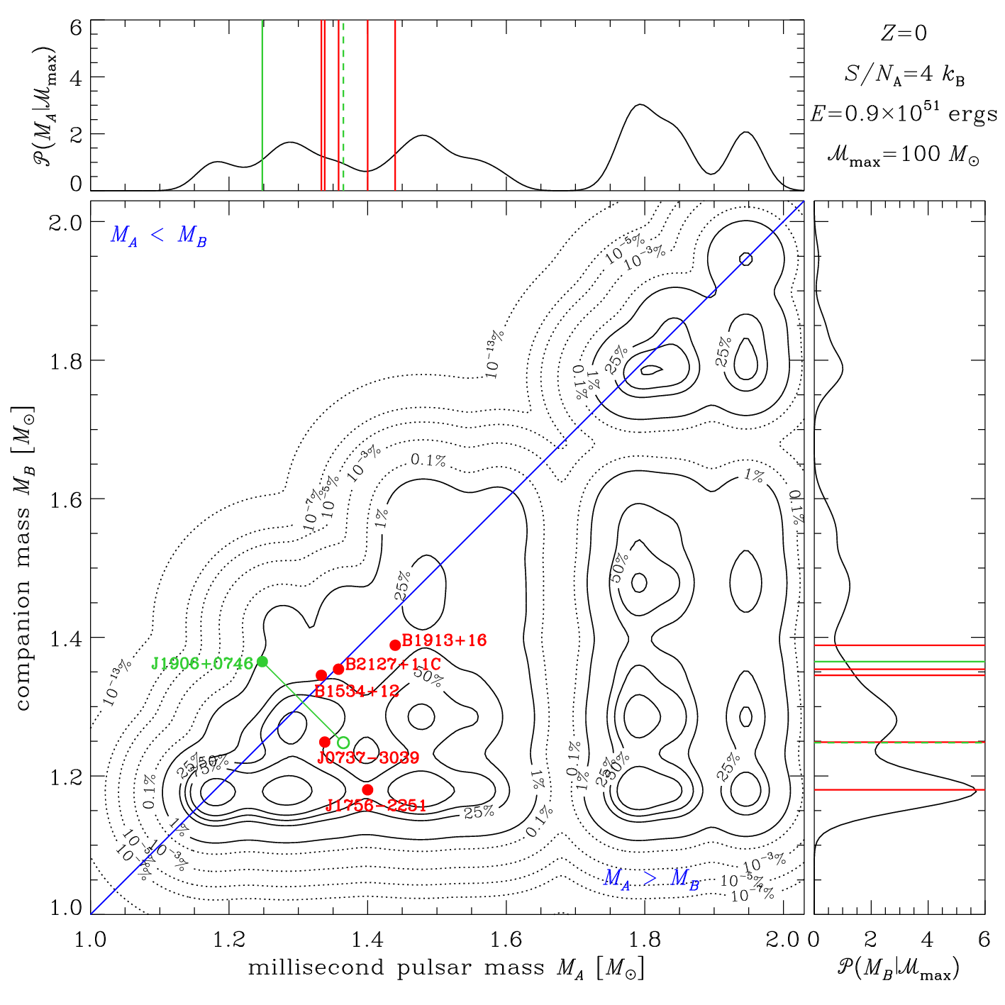
In Figures 1 and 2, we show examples of the probability distribution of NS masses originating from a binary $\mathscr{P}(M_{A},M_{B}|\mathscr{M}_{\rm max})$ with a uniform $P(q)$ along with the distributions marginalized over $M_{A}$ or $M_{B}$. The model in Figure 1 has the highest relative probability of all models considered in Section 3.2. For comparison, Figure 2 shows a model with fallback that has relative probability $B_{12}$ (Eq. [3]) lower by a factor of $\sim 10^{2.8}$. Examining Equation (8), we see that the primary and secondary mass ranges producing NS are quite different. For uniform $P(q)$, the probability distribution of primary masses $\mathscr{M}_{A}$ is proportional to $\mathscr{M}_{A}^{-\alpha}(1-\mathscr{M}_{\rm min}/\mathscr{M}_{A})$, and primaries with masses close to $\mathscr{M}_{\rm min}$ do not contribute to the distribution of NS masses $M_{A}$ because these systems mostly produce NS-WD binaries. The primary distribution producing NSs peaks at $(\alpha+1)\mathscr{M}_{\rm min}/\alpha\approx 1.43\mathscr{M}_{\rm min}$ for a Salpeter IMF. The distribution of secondaries producing NSs is proportional to $\mathscr{M}_{B}^{-\alpha}-\mathscr{M}_{\rm max}^{-\alpha}$ for a flat $P(q)$. Here, the cutoff is at high masses, while the distribution of the lowest mass progenitors is almost Salpeter. These analytic estimates immediately show that NS masses originating from the primary and secondary stars of a binary represent different progenitor mass ranges. For example, for $\mathscr{M}_{\rm min}=9.1\,M_{\odot}$ and $\mathscr{M}_{\rm max}=25\,M_{\odot}$, the mean progenitor masses of the primary and secondary components are $16.5$ and $12.8\,M_{\odot}$. This explains why the marginal distribution of $M_{A}$ in Figure 1 is not peaked at low $M_{A}$ and has a stronger secondary peak at $M_{A}\sim 1.6\,M_{\odot}$, when compared to the distribution of $M_{B}$. The secondary peak is much higher for models that include fallback (Fig. 2). There are no observed DNSs with masses in this second peak, which leads to a preference for models with no fallback (Section 3.2). The secondaries $\mathscr{M}_{B}$ have progenitor distributions close to the IMF. Thus, the highest peak for secondaries is at $1.22\,M_{\odot}$, which is the assumed gravitational NS mass for stars with $9.1\leq\mathscr{M}\leq 12\,M_{\odot}$.

We see from Figures 1 and 2 that most of the probability is in the region where the primary produces a more massive NS. However, since $M^{\prime}(\mathscr{M})$ is not monotonic (Zhang et al., 2008), there is a small probability that the more massive NS originated in fact from the less massive progenitor. Generally, the farther the NS mass pair is from the diagonal ($M_{A}=M_{B}$), the smaller the probability that the more massive NS came from the less massive progenitor. In our formalism we can estimate whether the mass difference between the two NSs is enough to distinguish between an NS originating from the primary or the secondary, or essentially whether the prior $P(p_{i})=\delta(p_{i}-1)$ in Equation (6) is appropriate. Figure 3 shows the ratio of probabilities that the millisecond pulsar originated from the more massive progenitor, $\mathscr{P}(M_{1},M_{2}|\mathscr{M}_{\rm max})$, as compared to the reverse $\mathscr{P}(M_{2},M_{1}|\mathscr{M}_{\rm max})$. In Figure 3 we have marginalized over explosion energies and $\mathscr{M}_{\rm max}$. We see that if $|M_{1}-M_{2}|\lesssim 2\sigma_{\rm theo}$, our model cannot distinguish between the primary/secondary origin of the millisecond pulsar based on the masses alone. The case of J1906$+$0746 is peculiar (because the pulsar is significantly less massive than the companion) and our results show that it is unlikely to have originated from the more massive progenitor. In agreement with Lorimer et al. (2006) who give a very small characteristic pulsar age (see also our Table 2), we propose that the observed pulsar in J1906$+$0746 comes from the less massive secondary star and we set the prior on $p_{i}$ in Equation (6) to be $P(p_{i})=\delta(p_{i})$ for this system. We show this alternative assignment as an open circle and the dashed lines in Figure 1. This alternative assignment increases the relative probability of the binary models by a factor of $\sim 3$ to $\sim 300$.

Next we evaluate the relative probabilities of individual models. We specifically discuss the differences between the independent and binary models, the explosion energy, and the position of the piston. We find that there is little difference in relative probability between the uniform and twin mass ratio distributions so we only discuss the uniform $P(q)$ model, which has slightly higher probability for solar metallicity. By comparing the relative probabilities of models with free $\mathscr{M}_{\rm max}$ to models that include all progenitors (equivalent to setting $P(\mathscr{M}_{\rm max})=\delta(\mathscr{M}_{\rm max}-100\,M_{\odot})$ in Eq. [3]), we also find that models with $\mathscr{M}_{\rm max}$ as a free parameter are not significantly preferred. The inferred values of $\mathscr{M}_{\rm max}$ range from $14\,M_{\odot}$ to $35\,M_{\odot}$ depending on the method used to infer the “best-fit” value, but with confidence intervals covering most of the allowed range for $\mathscr{M}_{\rm max}$. Here, we show models marginalized over $\mathscr{M}_{\rm max}$, although models simply fixing $\mathscr{M}_{\rm max}=100\,M_{\odot}$ give essentially the same results. Finally, for the purposes of this Section, we do the calculations with the pulsar in J1906$+$0746 attributed to the secondary star, consistent with Lorimer et al. (2006) and our discussion in Section 3.1.

Figure 4 shows the relative probabilities (Bayes factors) of our models as a function of explosion energy. Focusing first on the primordial composition models (left panel of Fig. 4), we see a general trend of increasing model probability for explosion energies up to about $E\approx 2\times 10^{51}$ ergs, after which the relative probability is essentially constant. The explanation is that higher $E$ explosions produce less fallback and hence reduce the number of high-mass NSs that expand the overall NS mass range. This is confirmed by the models that include only the mass of the core with no fallback (horizontal lines in Figure 4) that match the probabilities of the high-$E$ models. For solar composition (right panel of Fig. 4), the effect of $E$ is not clear. Since Zhang et al. (2008) investigated only two values of $E$, the probability ratios are not large (factor of $\sim 3$).

In all cases, the relative probabilities for binary versus independent mass models is between $5$ and $200$, which suggests a strong preference for binary models unless we assume that the pulsar in J1906$+$0746 came from the initially more massive star. In this case, the relative probability of the binary models decreases to a factor of $\sim 3$ for $Z=0$ and for $Z=Z_{☉}$ some of the models even disfavor the binary models. This relative change was expected based on Figure 3. If we assume uniform $P(p_{i})$ in Equation (6), the relative probability of binary models is again only a factor of $\sim 3$ higher than for the independent mass model. Binary models are significantly punished if there is a system with $M_{A}$ significantly lighter than $M_{B}$ if that is not allowed by the underlying remnant mass model. Correct treatment of the primary/secondary assignment of the millisecond pulsar and companion is crucial for properly evaluating the relative probabilities of the independent and binary models.

Figure 4 also shows clear differences in the relative probabilities of the different piston positions. For $Z=0$, the pistons at the $Y_{\rm e}$ core are strongly disfavored, because for low-mass progenitors the masses of the $Y_{\rm e}$ cores are too low. For solar composition, the situation is reversed. Models with the piston at the $Y_{\rm e}$ core are significantly more likely than those putting it at $S/N_{\rm A}=4\,k_{\rm B}$, because they reduce the number of NSs with $M>1.5\,M_{\odot}$. Furthermore, we see that the highest probability models essentially correspond to those with no fallback. There are small changes in the relative probabilities between the two binary mass ratio distributions ($P(q)$) and the primary/secondary assignment for J1906$+$0746. But the best overall model is the one with no fallback, uniform $P(q)$, and remnant masses equal to the $Y_{\rm e}$ core mass. The two piston positions used by Zhang et al. (2008) are somewhat arbitrary, so in Section 4 we address the question of whether some other piston position would produce better agreement with the observations.

While in the rest of this paper we examine the relative probability of different hypotheses for the DNS mass distribution in the Bayesian sense, at this point we make a “frequentist” diversion and compare the observations to the models in an absolute sense. We have argued that the individual NS masses in a DNS system reflect the binarity of the original system in the sense that the primary and secondary progenitor and NS mass distributions are different. Even though one of the components is observed as a pulsar, the ambiguity of which component originated from the primary or secondary star of the binary remains present for some systems unless more information is added (J1906$+$0746). In order to compare the models globally, we construct in Figure 5 cumulative distributions of the DNS total mass ($M_{1}+M_{2}$) and the mass difference ($|M_{1}-M_{2}|$), along with the predictions from Zhang et al. (2008) models coupled to the scenarios described in Section 2 with $\mathscr{M}_{\rm max}=100\,M_{\odot}$.

The distribution of mass differences in the left column of Figure 5 shows that getting the observed mass differences is entirely within the range of the models, although most of them predict a much broader distribution of mass differences. The twin models (blue and green lines) generally give smaller mass differences than their uniform $P(q)$ counterparts. Note that the no fallback, $Y_{\rm e}$ core, solar metallicity model with the highest Bayesian relative probability (thick yellow dashed line in the lower left panel) shows almost perfect agreement with the observations. We see in the cumulative distribution of total masses in the right column of Figure 5 that the observed distribution is much narrower than all theoretical predictions. The narrowest cumulative distributions are again produced by solar metallicity models with no fallback and remnant masses given by the $Y_{\rm e}$ core masses (thick dashed lines). Implementing a cutoff for progenitor mass $\mathscr{M}_{\rm max}$ makes the distributions narrower. However, this is only weakly favored by the observations. Additionally, the observed minimum total mass of $\sim 2.6\,M_{\odot}$ is markedly higher than any of the minimum total masses predicted by the models ($2.2$ to $2.4\,M_{\odot}$). The shift is $0.2$ to $0.3\,M_{\odot}$, which is much higher than the mass necessary to recycle the pulsar to the observed spin periods.

At this point in a “frequentist” analysis, we would compare the two cumulative distributions using a Kolmogorov-Smirnov test to ascertain whether the observations are compatible with the models in an absolute sense. However, mass differences and total masses are only particular aspects of the full 2D distributions. If we examine Figure 1, which shows $\mathscr{P}(M_{1},M_{2}|\mathscr{M}_{\rm max}=100\,M_{\odot})$ for the model with the highest Bayesian relative probability, we see that all $6$ binaries lie within the probability contour containing $75\%$ of the probability (if we assume that the pulsar in J1906$+$0746 came from the initially less massive progenitor). The chance of having no system outside this contour is $0.75^{6}=0.178$ and we would typically expect $4.5\pm 1.1$ systems within this contour given $6$ systems. This suggests that the highest Bayesian probability model represents the data quite well – the fact that there is no DNS system with $M>1.5\,M_{\odot}$ is likely only a statistical fluctuation. However, none of the three additional DNS systems with accurate total masses (Fig. 5, right panels) has a total mass of about $2.4\,M_{\odot}$, which suggests that the finer features of the DNS mass distribution might not be entirely reflected in the theoretical models. More DNS systems with accurate masses of both components are necessary to address this question.

There are numerous possible extensions to the analyses presented in this paper. For example, if $\mathscr{M}_{\rm min}$ is slightly lower, as suggested by studies of Type IIp supernova progenitors (Smartt, 2009), stars in this mass range will dominate the total probability due to the steepness of the Salpeter IMF. Core masses of the progenitors that were not explicitly calculated ($\mathscr{M}<10\,M_{\odot}$ for $Z=0$ and $\mathscr{M}<12\,M_{\odot}$ for $Z=Z_{☉}$) can also be different – Nomoto (1984) calculated presupernova structure of a $8.8\,M_{\odot}$ star, which has enclosed mass at both $S/N_{\rm A}=4\,k_{\rm B}$ and $Y_{\rm e}=0.499$ of $1.49\,M_{\odot}$ (baryonic)⁴⁴ 4 Note that in this model $S/N_{\rm A}<4\,k_{\rm B}$ for all zones below $1.49\,M_{\odot}$ except a single zone at $1.19\,M_{\odot}$, where it reaches $S/N_{\rm A}=4.02\,k_{\rm B}$., which is significantly higher than that assumed for low-mass progenitors in the Zhang et al. (2008) models. If we vary $\mathscr{M}_{\rm min}\geq 5\,M_{\odot}$ and the baryonic remnant mass of $1.2\leq M_{\rm ec}\leq 1.55\,M_{\odot}$ for stars where the progenitor structure was not explicitly calculated, use uniform priors in $\ln\mathscr{M}_{\rm min}$ and $\ln M_{\rm ec}$, and hold $\mathscr{M}_{\rm max}=100\,M_{\odot}$ fixed, we find very little change in the relative probabilities of the models. There is no significant change of $M_{\rm ec}$ with respect to Zhang et al. (2008). The results on the minimum progenitor mass are typically $\mathscr{M}_{\rm min}=8.9^{+1.4}_{-1.5}\,M_{\odot}$, which is compatible with both Zhang et al. (2008) and Smartt (2009). We also find $1.32\lesssim M_{\rm ec}\lesssim 1.39\,M_{\odot}$ for $Z=Z_{☉}$, which is compatible with Zhang et al. (2008).

The current DNS sample has only six systems with precise masses. A precise measurement of a NS birth mass greater than about $1.5\,M_{\odot}$ would greatly constrain the NS formation models. Until such system is found⁵⁵ 5 NS masses greater than $1.5\,M_{\odot}$ have been measured. For example, the system J1614$-$2230 has $M=1.97\pm 0.04\,M_{\odot}$ (Demorest et al., 2010). However, these NSs are likely significantly recycled and do not represent NS birth masses, although Lin et al. (2011) and Tauris et al. (2011) argue that the birth mass of J1614$-$2230 was higher than $1.5\,M_{\odot}$., it might be possible to obtain additional constraints by including NS systems with less precise mass measurements. The Bayesian formalism naturally accounts for non-Gaussian marginal likelihoods $P_{i}(\mathbf{D}|M)$ such as those presented by Özel et al. (2012) for some systems. Adding DNS systems with only a precise total mass measurement is unlikely to change our results, as their total masses are compatible with our sample (Fig. 5). We experimented with adding the eclipsing X-ray pulsars, which should also have masses near the birth mass (Rawls et al., 2011; Özel et al., 2012), and found that these measurements have uncertainties that are too large to improve the constraints.

The models can also be extended to include other types of binaries with degenerate components (e.g. BH-NS, BH-BH, NS-WD) since we can calculate the full remnant mass function for the binaries (Eq. [8]). That there are no known BH-NS binaries must strongly constrain $\mathscr{M}_{\rm max}$ through the relative probabilities of NS-NS, NS-BH and BH-BH for different values of $\mathscr{M}_{\rm max}$. Unfortunately, this also requires estimates for the relative detection efficiencies of the individual channels.

Finally, there are also a number of limitations to this work. The current sample of DNSs with precise masses has only six systems. The best available remnant mass function of Zhang et al. (2008) is based on 1D models that artificially explode non-rotating progenitors produced by a single stellar evolution code (Woosley et al., 2002). In addition, specific conditions have to be met to produce a DNS system. Belczynski et al. (2002) gives a comprehensive list of possible channels for DNS formation. Most of them involve mass transfer and a theoretically uncertain phase of common envelope evolution, which exposes the NS to potentially hypercritical accretion (Chevalier, 1993; Brown, 1995; Dewi et al., 2006; Lombardi et al., 2011, e.g.). Furthermore, Belczynski et al. (2010) investigated the relative numbers of DNS systems and isolated recycled pulsars and found a disagreement with theoretical predictions that point to a lack of understanding of massive binary star evolution or supernova explosions. Another significant effect is the disruption of binaries due to mass ejection and kicks during the two supernovae. We implemented the binary survival probability after the first supernova explosion by modifying Equation (8) using the results of Kalogera (1996). We used the final progenitor mass of Zhang et al. (2008) for the mass of the primary star before the explosion and various combinations of the initial and final mass for the secondary at the moment of the primary explosion. We also tried a number of relative kick velocities. Adding this to the calculation had no significant consequence. We note, however, that the second supernova is more important for the survival of the system (Dewi & van den Heuvel, 2004; Willems & Kalogera, 2004; Willems et al., 2004; Stairs et al., 2006; Wang et al., 2006; Wong et al., 2010, e.g.). Finally, while it is believed the NS masses are little affected by mass transfer, this may not hold for the progenitor stars. However, we think that results of detailed binary evolution and population synthesis models can affect only the details of the DNS mass distribution and not the overall conclusions.

References

- Akiyama et al. (2003) Akiyama, S., Wheeler, J. C., Meier, D. L., & Lichtenstadt, I. 2003, ApJ, 584, 954
- Arnett (1980) Arnett, W. D. 1980, ApJ, 237, 541
- Belczynski et al. (2002) Belczynski, K., Kalogera, V., & Bulik, T. 2002, ApJ, 572, 407
- Belczynski et al. (2010) Belczynski, K., Lorimer, D. R., Ridley, J. P., & Curran, S. J. 2010, MNRAS, 407, 1245
- Bethe (1990) Bethe, H. A. 1990, Reviews of Modern Physics, 62, 801
- Bethe & Wilson (1985) Bethe, H. A., & Wilson, J. R. 1985, ApJ, 295, 14
- Bhattacharya & van den Heuvel (1991) Bhattacharya, D., & van den Heuvel, E. P. J. 1991, Phys. Rep., 203, 1
- Brown & Bethe (1994) Brown, G. E., & Bethe, H. A. 1994, ApJ, 423, 659
- Brown (1995) Brown, G. E. 1995, ApJ, 440, 270
- Buras et al. (2006a) Buras, R., Rampp, M., Janka, H.-T., & Kifonidis, K. 2006, A&A, 447, 1049
- Buras et al. (2006b) Buras, R., Janka, H.-T., Rampp, M., & Kifonidis, K. 2006, A&A, 457, 281
- Burgay et al. (2003) Burgay, M., D’Amico, N., Possenti, A., et al. 2003, Nature, 426, 531
- Burrows (1986) Burrows, A. 1986, ApJ, 300, 488
- Burrows et al. (1995) Burrows, A., Hayes, J., & Fryxell, B. A. 1995, ApJ, 450, 830
- Burrows & Goshy (1993) Burrows, A., & Goshy, J. 1993, ApJ, 416, L75
- Burrows et al. (2007) Burrows, A., Dessart, L., Livne, E., Ott, C. D., & Murphy, J. 2007, ApJ, 664, 416
- Champion et al. (2005) Champion, D. J., Lorimer, D. R., McLaughlin, M. A., et al. 2005, MNRAS, 363, 929
- Chevalier (1976) Chevalier, R. A. 1976, ApJ, 207, 872
- Chevalier (1989) Chevalier, R. A. 1989, ApJ, 346, 847
- Chevalier (1993) Chevalier, R. A. 1993, ApJ, 411, L33
- Colgate & White (1966) Colgate, S. A., & White, R. H. 1966, ApJ, 143, 626
- Corongiu et al. (2007) Corongiu, A., Kramer, M., Stappers, B. W., et al. 2007, A&A, 462, 703
- Demorest et al. (2010) Demorest, P. B., Pennucci, T., Ransom, S. M., Roberts, M. S. E., & Hessels, J. W. T. 2010, Nature, 467, 1081
- Dessart et al. (2008) Dessart, L., Burrows, A., Livne, E., & Ott, C. D. 2008, ApJ, 673, L43
- Dessart et al. (2011) Dessart, L., Hillier, D. J., Livne, E., et al. 2011, MNRAS, 414, 2985
- Dessart et al. (2012) Dessart, L., O’Connor, E., & Ott, C. D. 2012, arXiv:1203.1926
- Dewi & van den Heuvel (2004) Dewi, J. D. M., & van den Heuvel, E. P. J. 2004, MNRAS, 349, 169
- Dewi et al. (2006) Dewi, J. D. M., Podsiadlowski, P., & Sena, A. 2006, MNRAS, 368, 1742
- Eldridge et al. (2011) Eldridge, J. J., Langer, N., & Tout, C. A. 2011, MNRAS, 414, 3501
- Faulkner et al. (2005) Faulkner, A. J., Kramer, M., Lyne, A. G., et al. 2005, ApJ, 618, L119
- Fernández (2012) Fernández, R. 2012, ApJ, 749, 142
- Finn (1994) Finn, L. S. 1994, Physical Review Letters, 73, 1878
- Fryer & Heger (2000) Fryer, C. L., & Heger, A. 2000, ApJ, 541, 1033
- Fryer & Warren (2002) Fryer, C. L., & Warren, M. S. 2002, ApJ, 574, L65
- Fryer & Warren (2004) Fryer, C. L., & Warren, M. S. 2004, ApJ, 601, 391
- Fryer et al. (2012) Fryer, C. L., Belczynski, K., Wiktorowicz, G., et al. 2012, ApJ, 749, 91
- Fujimoto et al. (2011) Fujimoto, S.-i., Kotake, K., Hashimoto, M.-a., Ono, M., & Ohnishi, N. 2011, ApJ, 738, 61
- Georgy (2012) Georgy, C. 2012, A&A, 538, L8
- Goldreich & Weber (1980) Goldreich, P., & Weber, S. V. 1980, ApJ, 238, 991
- Hanke et al. (2011) Hanke, F., Marek, A., Müller, B., & Janka, H.-T. 2011, arXiv:1108.4355
- Heger et al. (2003) Heger, A., Fryer, C. L., Woosley, S. E., Langer, N., & Hartmann, D. H. 2003, ApJ, 591, 288
- Herant et al. (1992) Herant, M., Benz, W., & Colgate, S. 1992, ApJ, 395, 642
- Herant et al. (1994) Herant, M., Benz, W., Hix, W. R., Fryer, C. L., & Colgate, S. A. 1994, ApJ, 435, 339
- Iwakami et al. (2008) Iwakami, W., Kotake, K., Ohnishi, N., Yamada, S., & Sawada, K. 2008, ApJ, 678, 1207
- Jacoby et al. (2006) Jacoby, B. A., Cameron, P. B., Jenet, F. A., et al. 2006, ApJ, 644, L113
- Janka & Müller (1996) Janka, H.-T., & Müller, E. 1996, A&A, 306, 167
- Janka et al. (2007) Janka, H.-T., Langanke, K., Marek, A., Martínez-Pinedo, G., Müller, B. 2007, Phys. Rep., 442, 38
- Janssen et al. (2008) Janssen, G. H., Stappers, B. W., Kramer, M., et al. 2008, A&A, 490, 753
- Jeffreys (1983) Jeffreys, H. 1983, The Theory of Probability, 3rd ed., Oxford University Press
- Juneau et al. (2005) Juneau, S., Glazebrook, K., Crampton, D., et al. 2005, ApJ, 619, L135
- Kalogera (1996) Kalogera, V. 1996, ApJ, 471, 352
- Kasian (2008) Kasian, L. 2008, 40 Years of Pulsars: Millisecond Pulsars, Magnetars and More, 983, 485
- Keil & Janka (1995) Keil, W., & Janka, H.-T. 1995, A&A, 296, 145
- Kitaura et al. (2006) Kitaura, F. S., Janka, H.-T., & Hillebrandt, W. 2006, A&A, 450, 345
- Kiziltan et al. (2010) Kiziltan, B., Kottas, A., & Thorsett, S. E. 2010, arXiv:1011.4291
- Kobulnicky & Fryer (2007) Kobulnicky, H. A., & Fryer, C. L. 2007, ApJ, 670, 747
- Kochanek et al. (2008) Kochanek, C. S., Beacom, J. F., Kistler, M. D., et al. 2008, ApJ, 684, 1336
- Kochanek (2009) Kochanek, C. S. 2009, ApJ, 707, 1578
- Kotake et al. (2011) Kotake, K., Iwakami-Nakano, W., & Ohnishi, N. 2011, ApJ, 736, 124
- Kramer et al. (2006) Kramer, M., Stairs, I. H., Manchester, R. N., et al. 2006, Science, 314, 97
- Kuroda et al. (2012) Kuroda, T., Kotake, K., & Takiwaki, T. 2012, arXiv:1202.2487
- Lattimer & Yahil (1989) Lattimer, J. M., & Yahil, A. 1989, ApJ, 340, 426
- Levesque et al. (2005) Levesque, E. M., Massey, P., Olsen, K. A. G., et al. 2005, ApJ, 628, 973
- Liebendörfer et al. (2001) Liebendörfer, M., Mezzacappa, A., Thielemann, F.-K., et al. 2001, Phys. Rev. D, 63, 103004
- Lin et al. (2011) Lin, J., Rappaport, S., Podsiadlowski, P., et al. 2011, ApJ, 732, 70
- Lombardi et al. (2011) Lombardi, J. C., Jr., Holtzman, W., Dooley, K. L., et al. 2011, ApJ, 737, 49
- Lorimer et al. (2006) Lorimer, D. R., Stairs, I. H., Freire, P. C., et al. 2006, ApJ, 640, 428
- Lyne et al. (2004) Lyne, A. G., Burgay, M., Kramer, M., et al. 2004, Science, 303, 1153
- MacFadyen et al. (2001) MacFadyen, A. I., Woosley, S. E., & Heger, A. 2001, ApJ, 550, 410
- Marek & Janka (2009) Marek, A., & Janka, H.-T. 2009, ApJ, 694, 664
- Moriya et al. (2011) Moriya, T., Tominaga, N., Blinnikov, S. I., Baklanov, P. V., & Sorokina, E. I. 2011, MNRAS, 415, 199
- Müller et al. (2012) Müller, B., Janka, H.-T., & Marek, A. 2012, arXiv:1202.0815
- Murphy & Burrows (2008) Murphy, J. W., & Burrows, A. 2008, ApJ, 688, 1159
- Nomoto (1984) Nomoto, K. 1984, ApJ, 277, 791
- Nordhaus et al. (2010) Nordhaus, J., Burrows, A., Almgren, A., & Bell, J. 2010, ApJ, 720, 694
- Nordhaus et al. (2011) Nordhaus, J., Brandt, T., Burrows, A., & Almgren, A. 2011, arXiv:1112.3342
- O’Connor & Ott (2011) O’Connor, E., & Ott, C. D. 2011, ApJ, 730, 70
- Ohnishi et al. (2006) Ohnishi, N., Kotake, K., & Yamada, S. 2006, ApJ, 641, 1018
- Ott et al. (2004) Ott, C. D., Burrows, A., Livne, E., & Walder, R. 2004, ApJ, 600, 834
- Ott et al. (2012) Ott, C. D., Abdikamalov, E., O’Connor, E., et al. 2012, arXiv:1204:0512
- Özel et al. (2010) Özel, F., Psaltis, D., Narayan, R., & McClintock, J. E. 2010, ApJ, 725, 1918
- Özel et al. (2012) Ozel, F., Psaltis, D., Narayan, R., & Santos Villarreal, A. 2012, arXiv:1201.1006
- Pejcha & Thompson (2012) Pejcha, O., & Thompson, T. A. 2012, ApJ, 746, 106
- Pinsonneault & Stanek (2006) Pinsonneault, M. H., & Stanek, K. Z. 2006, ApJ, 639, L67
- Portegies Zwart & Yungelson (1998) Portegies Zwart, S. F., & Yungelson, L. R. 1998, A&A, 332, 173
- Press (1997) Press, W. H. 1997, in Unsolved Problems in Astrophysics, ed. J. N. Bahcall & J. P. Ostriker (Princeton, NJ), 49
- Rawls et al. (2011) Rawls, M. L., Orosz, J. A., McClintock, J. E., et al. 2011, ApJ, 730, 25
- Salpeter (1955) Salpeter, E. E. 1955, ApJ, 121, 161
- Scheck et al. (2006) Scheck, L., Kifonidis, K., Janka, H.-T., Müller, E. 2006, A&A, 457, 963
- Schwab et al. (2010) Schwab, J., Podsiadlowski, P., & Rappaport, S. 2010, ApJ, 719, 722
- Smartt (2009) Smartt, S. J. 2009, ARA&A, 47, 63
- Smartt et al. (2009) Smartt, S. J., Eldridge, J. J., Crockett, R. M., & Maund, J. R. 2009, MNRAS, 395, 1409
- Smith et al. (2009) Smith, N., Hinkle, K. H., & Ryde, N. 2009, AJ, 137, 3558
- Smith et al. (2011) Smith, N., Li, W., Filippenko, A. V., & Chornock, R. 2011, MNRAS, 412, 1522
- Stairs et al. (2002) Stairs, I. H., Thorsett, S. E., Taylor, J. H., & Wolszczan, A. 2002, ApJ, 581, 501
- Stairs et al. (2006) Stairs, I. H., Thorsett, S. E., Dewey, R. J., Kramer, M., & McPhee, C. A. 2006, MNRAS, 373, L50
- Suwa et al. (2010) Suwa, Y., Kotake, K., Takiwaki, T., et al. 2010, PASJ, 62, L49
- Symbalisty (1984) Symbalisty, E. M. D. 1984, ApJ, 285, 729
- Takiwaki et al. (2012) Takiwaki, T., Kotake, K., & Suwa, Y. 2012, ApJ, 749, 98
- Tauris et al. (2011) Tauris, T. M., Langer, N., & Kramer, M. 2011, MNRAS, 416, 2130
- Thielemann et al. (1996) Thielemann, F.-K., Nomoto, K., & Hashimoto, M.-A. 1996, ApJ, 460, 408
- Thompson et al. (2001) Thompson, T. A., Burrows, A., & Meyer, B. S. 2001, ApJ, 562, 887
- Thompson et al. (2005) Thompson, T. A., Quataert, E., & Burrows, A. 2005, ApJ, 620, 861
- Thorsett & Chakrabarty (1999) Thorsett, S. E., & Chakrabarty, D. 1999, ApJ, 512, 288
- Timmes et al. (1996) Timmes, F. X., Woosley, S. E., & Weaver, T. A. 1996, ApJ, 457, 834
- Ugliano et al. (2012) Ugliano, M., Janka, H.-T., Marek, A., & Arcones, A. 2012, arXiv:1205.3657
- Valentim et al. (2011) Valentim, R., Rangel, E., & Horvath, J. E. 2011, MNRAS, 414, 1427
- Wang et al. (2006) Wang, C., Lai, D., & Han, J. L. 2006, ApJ, 639, 1007
- Weisberg et al. (2010) Weisberg, J. M., Nice, D. J., & Taylor, J. H. 2010, ApJ, 722, 1030
- Willems & Kalogera (2004) Willems, B., & Kalogera, V. 2004, ApJ, 603, L101
- Willems et al. (2004) Willems, B., Kalogera, V., & Henninger, M. 2004, ApJ, 616, 414
- Wong et al. (2010) Wong, T.-W., Willems, B., & Kalogera, V. 2010, ApJ, 721, 1689
- Woosley & Weaver (1995) Woosley, S. E., & Weaver, T. A. 1995, ApJS, 101, 181
- Woosley et al. (2002) Woosley, S. E., Heger, A., & Weaver, T. A. 2002, Reviews of Modern Physics, 74, 1015
- Yahil (1983) Yahil, A. 1983, ApJ, 265, 1047
- Yamasaki & Yamada (2005) Yamasaki, T., & Yamada, S. 2005, ApJ, 623, 1000
- Yamasaki & Yamada (2006) Yamasaki, T., & Yamada, S. 2006, ApJ, 650, 291
- Yoon & Cantiello (2010) Yoon, S.-C., & Cantiello, M. 2010, ApJ, 717, L62
- Yüksel & Beacom (2007) Yüksel, H., & Beacom, J. F. 2007, Phys. Rev. D, 76, 083007
- Zhang et al. (2008) Zhang, W., Woosley, S. E., & Heger, A. 2008, ApJ, 679, 639
- Zhang et al. (2011) Zhang, C. M., Wang, J., Zhao, Y. H., et al. 2011, A&A, 527, A83
Appendix A The NS mass distribution of Ugliano et al. (2012)
After the submission of this paper, Ugliano et al. (2012) published a NS mass distribution that is based on 1D simulations of neutrino-driven explosions followed from the onset of the collapse until the end of the fallback. The simulations are normalized by comparison with the observed parameters of SN 1987A. The distribution is based on over progenitors with , which we supplement with remnant masses of for , similarly to the models of Zhang et al. (2008) discussed in the main paper. We also corrected the remnant masses for the binding energy according to Equation (9). In Figure 7, we show the resulting probability distribution of the DNS masses. We see that the peaks of the distribution are shifted by to higher masses with the respect to the DNS data. Even though the fallback on the remnants is included, the probability distribution has little power for NS masses higher than about , unlike the large amounts of fallback in many of the Zhang et al. (2008) models (Fig. 2). Indeed, Ugliano et al. (2012) find little fallback for high-mass progenitors.
In order to compare the relative probability of the Ugliano et al. (2012) distribution to the models in Figure 6, we marginalize over and the remnant mass for progenitors with in the same way as we did for the models of Woosley et al. (2002). We find that the relative probability is only on the scale of Figure 6, which is likely caused by the slight mismatch in the probability peaks with respect to the DNS data. If we include remnant masses without fallback, which might be more appropriate for DNS progenitors with stripped hydrogen envelopes, the relative probability raises to about . However, this is about a factor of worse than our best models in Figures 4 and 6. Thus, the reduction of fallback in the Ugliano et al. (2012) NS mass distribution provides a better match to the observed masses of DNS binaries, but not as good match as the Zhang et al. (2008) core models with no fallback.