One dimensional -wave holographic superconductor with supercurrent
Abstract:
We study the one dimensional -wave holographic superconductor by turning on the vector potential in the bulk, which behaves as on the boundary. By solving the model with fixed , we find that if we identify the with the supercurrent of the holographic superconductor, the results agree with the Ginzburg- Landau theory. For example, will break the superconductivity, and the critical value of is proportional to .
Keywords:
Holography, Superconductivity, AdS3/CFT21 Introduction
The AdS/CFT correspondence [1, 2, 3, 4] has been taken as a very useful method to study strongly coupled phenomena now. A successful application of the AdS/CFT correspondence to condensed matter physics is to study the superconductors. The strategy to build a holographic superconductor is to couple an black hole with some charged field and the gauge fields. The black hole will have hair when the temperature of the black hole is low enough. The charged hair breaks the gauge symmetry in the bulk and the black hole is superconducting [5]. By putting a charged scalar field coupled to the gauge field in black hole, one can get the -wave holographic superconductor in which the order parameter is a scalar[6, 7]. By putting a pure gauge field in the bulk theory, one can get the -wave holographic superconductor with a vector order parameter [8, 9, 10, 11, 12]. In order to build a -wave holographic superconductor we need a charged tensor field coupled to a gauge field in the bulk that leads to a tensor order parameter [13, 14, 15].
Most of the studies on holographic superconductors have focused on the dimensional systems by using AdS4/CFT3. The dimensional holographic superconductor shows similar properties as the dimensional superconductors, as studied in[16] by using AdS5/CFT4. The dimensional -wave and -wave holographic superconductors were explored in [17] and [18] respectively by using AdS3/CFT2. Due to the logarithm behavior of on the boundary, we have to realize that the AdS3 realization of holographic superconductor is an honest superconductor with a dynamic gauge field on the boundary, in which the local boundary symmetry is spontaneously broken [18]. The holographic superconductors with dynamic gauge fields in higher dimensions were studied in [19, 20, 21, 22]. A holographic quantum liquid in (1+1) dimensions from a probe D3 brane in the AdS Schwarzschild planar black hole background was studied in [23].
In this paper, we studied the one dimensional -wave holographic superconductor by switching on the vector potential in the bulk theory. behaves as on the AdS3 boundary. By solving the model with fixed , we find that plays the role of supercurrent in a superconductor. If we identify with the supercurrent and as the superfluid velocity , the results agree with the Ginzburg- Landau (G-L) theory for a superconductor with supercurrent. For example, will break the superconductivity, the critical value of being proportional to . These results indicate that we can interpret the source term as the supercurrent while as the superfluid velocity . The G-L theory results we found in dimensional -wave holographic superconductors have also been founded in the dimensional holographic superconductors with supercurrent[24]. In analogy, for the scalar potential on the boundary, can be interpreted as the charge density while as the chemical potential .
The organization of this paper is as follows. In Section we first introduce the Einstein-Maxwell-charged scalar system in AdS3 black hole, and then confirm that there is a continuous phase transition when by free energy calculations. In Section we solve the system with fixed value of and we find that should be the supercurrent of the holographic superconductor. We also try to solve the system with fixed value of in Section . Discussions and conclusions are given in Section .
2 The condensed phase with
In this section we firstly review the results in [17]. We also compute the free energy to confirm the existence of the continuous superconducting phase transition.
2.1 The Einstein-Maxwell-charged scalar system in black hole
The Lagrangian of the Einstein-Maxwell-charged scalar system reads
| (1) |
The neutral black hole background in Poincaré coordinates is given by [17]
| (2) |
in which , , and is the horizon of the black hole. We set and . The black hole temperature is given by
| (3) |
With the ansatz
| (4) |
we have the equations of motion (EOMs) for the three fields,
| (5) |
| (6) |
| (7) |
The boundary behavior for the two Maxwell fields and at are
| (8) |
| (9) |
where is the renormalization scale included in the logarithm. We set to be without loss of generality. It has been found that there is only one way to quantize the theory (alternative quantization) by defining the coefficients of the logarithmic terms to be the sources [25, 26, 27].
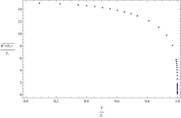
As for the scalar field , we can only consider the case of , since the results for other values of are similar [17]. The asymptotic behavior of near the boundary for reads
| (10) |
We can only choose the scalar operator as , with the boundary condition [17]. is the order parameter of the superconductor. On the horizon, regularity requires , with the other two fields and being finite. In this section we set and solve the two EOMs Eq. (2.5) and Eq. (2.6) for and with vanishing .
2.2 Phase diagram and the free energy analysis
The phase diagram of the superconductor with is plotted in Fig. 1. It is clear that there is a continuous phase transition at . After computing the free energy density we will confirm the result further.
According to the AdS/CFT dictionary, the free energy of the dual field theory is related to the on-shell action of the classical gravity theory,
| (11) |
where the ellipsis denotes boundary terms we may need. Employing the equations of motion, the on-shell action can be written as
| (12) |
By plugging in the asymptotic behaviors of , and we get
| (13) |
In order work in the ensemble with fixed , we need to add the boundary [25, 26]
| (14) |
where is the induced metric of the boundary. We can see which is divergent. In order to cancel the divergence, we add the counter term[26]
| (15) |
Finally, the free energy density for the superconductor reads
| (16) |
where is the length of the superconducting wire. The superconductor is uniform since the order parameter is independent of .

In Fig. 2 we plot the free energy density difference between the superconducting and normal states. It can be seen that the superconducting state is more stable than the normal state when .
3 The superconductor with fixed
In AdS4 setup of holographic superconductor, on the boundary. It is clear now we can interpret as the superfluid velocity and as the supercurrent. There are two kinds of quantizations for , which means that we can fix the value of and let free to fluctuate, or fix the value of and let free to fluctuate. The two methods to solve the problem correspond to experiments where the current, or the superfluid velocity is kept fixed. It has been shown [24, 28, 29, 30] that by fixing or on the boundary, the black hole holographic superconductors (both -wave and -wave holographic superconductors) with fixed supercurrent or fixed superfluidity velocity have the same results as G-L theory.
However, since the gauge fields behave much differently on AdS3 boundary, it is very interesting to ask what will happen when the superconducting black hole has non-vanishing vector potential . In this section we solve the EOMs with fixed value of in Eq. (2.9). In the next section we also try to solve the EOMs with fixed value of in Eq. (2.9).
3.1 The condensate versus temperature
The first important problem to study is how the order parameter changes with the temperature for this holographic superconductor with fixed . From now on we suppose is the supercurrent and is the superfluid velocity . From Fig. 3 it can be seen that when the supercurrent is not zero, there are two solutions of the order parameter corresponding to a fixed temperature. We also show that the solution with lower value of the order parameter takes a larger free energy than the solution with larger values of the order parameter and therefore it is unfavorable. In Fig. 4 we present the free energy of a fixed current for the two branches of solution. It can be obviously seen that the solution with a larger value of the order parameter has a lower free energy. The critical temperature decreases when the current increases, which indicates that there should exist a critical current above which there is no superconductivity. When one lowers the temperature from above the critical temperature, the order of phase transition at the critical temperature for a fixed current should be of first order, since the order parameter jumps from zero to a finite value at the critical temperature. Such a jump will certainly change the energy and so requires some latent heat, which implies that the phase transition should be of first order. This conclusion is the same as the one we shall give by observing the curve of the current versus the superfluid velocity at a fixed temperature soon. For the -wave holographic superconductor with current, the order parameter is also bivalued, and the states with lower value of the condensate have a larger free energy than their counterparts with larger values of the condensate at the same temperature.[24]


3.2 Results that agree with the G-L theory
In this section we give more evidences that behaves the same as a supercurrent in a superconductor. These results indicate that we should interpret as the supercurrent in the boundary theory.
3.2.1 Current via the superfluid velocity
Another physical property by which one can compare the difference between the gravity model of superconductor and the G-L theory is the relation between the current and the superfluidity velocity at a fixed temperature. From this relation we can also get the information of the phase transition at the critical current.


The two plots in Fig. 5 correspond to the two temperatures and . For these two temperatures the critical currents are and , respectively. It can be clearly seen that at the temperatures close to , where the G-L theory works very well, the plots of versus are the same as that of G-L theory, in which the and have a linear relationship when is much smaller than . From these plots we can also infer the order of the phase transitions at critical current or critical velocity. For the two plots, the maximal velocity corresponds to a vanishing current, which means that the phase transitions at critical velocities the and are of second order. However, the maximal current corresponds to a non-vanishing velocity, which means that the phase transitions at critical currents and are of first order.
3.2.2 The critical current via temperature
In this subsection we study the critical current for different near to compare the results with those of the G-L theory. As predicted by G-L theory, is proportional to when the temperature is close to . As illustrated in Fig. 6, this scaling behavior is indeed obeyed by holographic superconductors for temperatures close to , which is also the case in the dimensional -wave model[24]. Another prediction of the G-L theory is that, at any fixed temperature, the norm of the condensate decreases monotonically with respect to the velocity from its maximal value. And the maximal value corresponds to zero velocity and zero current. As shown in Fig. 5, the critical current is reached before the velocity reaches its maximal value. The norm of the condensate has an intermediate value at the maximal current. The G-L theory tells us that the ratio of to is exactly . From Fig. 7 it can be seen that this is indeed the case for the dimensional -wave holographic superconductor.


4 The superconductor with fixed
Before we give the results when we solve the EOMs with fixed . We would like to emphasis that there is only one kind of quantization of the theory, we can only take is the source. However, fixing does not contradict the statement in [25], we are simply in another ensemble which can be changed to the ensemble in last section with fixed by a Legendre transformation[26]. From the numerical computation we find that to solve the EOMs with fixed is indeed much more difficult numerically, it will take very long time for the shooting method to give a solution. In Fig. 7 we give two samples of solutions for fixed and respectively. It can be seen that the phase transition with the small values of velocity is of second order, which confirms our discussion in section 3.2.1.


5 Conclusion
With the fact the Maxwell gauge fields and behave as in Eq. (2.8) and Eq. (2.9) on the boundary, and an important question arises as how to interpret the coefficients and . Formally, this question was already answered in [18, 25, 26], the source term is the charge density and is the chemical potential. In this paper we have confirm the conclusion given in [18, 25, 26] by studying the properties of the dimensional holographic superconductor with nonzero . By solving the EOMs we found that if we interpret and in Eq. (2.9) as the supercurrent and the superfluidity velocity respectively, the results near the critical temperature agree qualitatively with several properties of the Ginzburg-Landau theory:
- •
The phase transition with supercurrent is of first order
- •
The critical supercurrent is proportional to
- •
The relation between velocity and supercurrent is linear almost all the way up to a given maximum velocity
- •
The squared ratio of the maximal condensate to the minimal condensate is equal to two thirds
Furthermore, the in Eq. (2.8) is the charge density and is the chemical potential. We summarize these results as
| (17) |
and
| (18) |
on the boundary, where is the chemical potential, is the charge density, is the superfluid velocity and is the supercurrent.
We state that there should be a supercurrent in the dimensional holographic superconductor when we include in the bulk theory, which corresponds to the coefficient of the logarithmic term on the boundary (see Eq. (2.9)). The existence of supercurrent in a holographic superconductor means there should also be superconducting tunneling effect by building a holographic Josephson Junction.[31, 32, 33, 34] Then another way to confirm the conclusion that is the supercurrent is to find the holographic Josephson Junction in the setup of superconductors. We leave this for future work.
Acknowledgements
It is a pleasure to thank Xin Gao, Matthias Kaminski, Hai-Qing Zhang and Zhe-Yong Fan for valuable discussions. H. B. Zeng is supported by the Fundamental Research Funds for the Central Universities (Grant No. 1107020117) and the China Postdoctoral Science Foundation (Grant No. 20100481120).
References
- [1] J. M. Maldacena, “The large N limit of superconformal field theories and supergravity,” Adv. Theor. Math. Phys. 2 (1998) 231 [arXiv:hep-th/9711200].
- [2] S. S. Gubser, I. R. Klebanov and A. M. Polyakov, “Gauge Theory Correlators from Non-Critical String Theory,” Phys. Lett. B 428 (1998) 105 [arXiv:hep-th/9802109].
- [3] E. Witten, “Anti-de Sitter space and holography,” Adv. Theor. Math. Phys. 2 (1998) 253 [arXiv:hep-th/9802150].
- [4] O. Aharony, S. S. Gubser, J. M. Maldacena, H. Ooguri, and Y. Oz, “Large N Field Theories, String Theory and Gravity,” Phys. Rept. 323 (2000) 183 [arXiv:hep-th/9905111].
- [5] S. S. Gubser, “Breaking an Abelian gauge symmetry near a black hole horizon,”Phys. Rev. D 78 (2008) 065034 .
- [6] S. A. Hartnoll, C. P. Herzog and G. T. Horowitz, “Building a Holographic Superconductor,” Phys. Rev. Lett. 101 (2008) 031601 [arXiv:0803.3295 ].
- [7] S. A. Hartnoll, C. P. Herzog and G. T. Horowitz, “Holographic Superconductors,” JHEP 12 (2008) 015 [arXiv:0810.1563 [hep-th]].
- [8] S. S. Gubser, “Colorful horizons with charge in anti-de Sitter space,”Phys. Rev. Lett. 101 (2008) 191601 .
- [9] S. S. Gubser and S. S. Pufu, “The gravity dual of a p-wave superconductor,” JHEP 11 (2008) 033 [arXiv:0805.2960].
- [10] M. M. Roberts and S. A. Hartnoll, “Pseudogap and time reversal breaking in a holographic superconductor,” JHEP 08 (2008) 035 [arXiv:0805.3898].
- [11] M. Ammon, J. Erdmenger, M. Kaminski and P. Kerner, “Superconductivity from gauge/gravity duality with flavor,” Phys. Lett. B 680 (2009) 516 [arXiv:0810.2316].
- [12] M. Ammon, J. Erdmenger, M. Kaminski and P. Kerner, “Flavor Superconductivity from Gauge/Gravity Duality,” JHEP 10 (2009) 067 [arXiv:0903.1864].
- [13] Jiunn-Wei Chen, Ying-Jer Kao, Debaprasad Maity, Wen-Yu Wen, Chen-Pin Yeh,“Towards A Holographic Model of D-Wave Superconductors ,”Phys. Rev. D 81 (2010) 106008.
- [14] Francesco Benini, Christopher P. Herzog, and Amos Yarom, “Holographic Fermi arcs and a d-wave gap,” Phys. Lett. B 701 (2011) 626 [arXiv:1006.0731v1].
- [15] Francesco Benini, Christopher P. Herzog, Rakibur Rahman, Amos Yarom,“Gauge gravity duality for d-wave superconductors: prospects and challenges ” JHEP 11(2010) 137 [arXiv:1007.1981].
- [16] G. T. Horowitz and M. M. Roberts, “Holographic Superconductors with Various Condensates,”Phys. Rev. D 78 (2008) 126008 [arXiv:hep-th/0810.1077].
- [17] Jie Ren “One-dimensional holographic superconductor from correspondence,” JHEP 11 (2010)055 [arXiv:1008.3904v3].
- [18] Xin Gao, M. Kaminski, H. B. Zeng and H. Q. Zhang “Non-Equilibrium Field Dynamics of an Honest Holographic Superconductor , ” [arXiv:1204.3103].
- [19] O. Domenech, M. Montull, A. Pomarol, A. Salvio, and P. J. Silva, Emergent Gauge Fields in Holographic Superconductors, JHEP 08 (2010) 033, [arXiv:1005.1776].
- [20] M. Montull, O. Pujolas, A. Salvio, and P. J. Silva, Magnetic Response in the Holographic Insulator/Superconductor Transition, [arXiv:1202.0006].
- [21] P. J. Silva, Dynamical gauge fields in holographic superconductors, Fortsch.Phys. 59 (2011) 756¨C761.
- [22] M. Montull, O. Pujolas, A. Salvio, and P. J. Silva, Flux Periodicities and Quantum Hair on Holographic Superconductors, Phys.Rev.Lett. 107 (2011) 181601, [arXiv:1105.5392].
- [23] L.-Y. Hung and A. Sinha, “Holographic quantum liquids in 1+1 dimensions,” JHEP 01 (2010) 114, [arXiv:0909.3526].
- [24] Daniel Arean, Matteo Bertolini, Jarah Evslin, Tomas Prochazka,“On Holographic Superconductors with DC Current,” [arXiv:1003.5661].
- [25] D. Marolf and S. Ross, “Boundary conditions and dualities: vector fields in AdS/CFT,” JHEP 11 (2006) 085 [arXiv:hep-th/0606113].
- [26] Kristan Jensen, “Chiral anomalies and AdS/CMT in two dimensions ,” JHEP 01 (2011) 109 [arXiv:1012.4831v1].
- [27] T. Andrade, J. I. Jottar, and R. G. Leigh, “Boundary Conditions and Unitarity: the Maxwell-Chern-Simons System in ”, [arXiv:1111.5054].
- [28] C. P. Herzog, P. K. Kovtun and D. T. Son, “Holographic model of superfluidity,” Phys. Rev. D 79 (2009) 066002 [arXiv:0809.4870].
- [29] Pallab Basu, Anindya Mukherjee, Hsien-Hang Shieh, “Supercurrent: Vector Hair for an AdS Black Hole,” Phys. Rev. D 79 (2009) 045010 [arXiv:0809.449].
- [30] H. B. Zeng, W. M. Sun, H. S. Zong, “ Supercurrent in p-wave Holographic Superconductor ,” Phys. Rev. D 83 (2011) 046010 [arXiv:1010.5039].
- [31] Gary T. Horowitz, Jorge E. Santos, Benson Way, “A Holographic Josephson Junction,” Phys. Rev. Lett 106 (2011) 221601 [arXiv:1101.3326v4].
- [32] Yong-Qiang Wang, Yu-Xiao Liu, Zhen-Hua Zhao,“Holographic p-wave Josephson junction,” [arXiv:1109.4426].
- [33] Yong-Qiang Wang, Yu-Xiao Liu, Zhen-Hua Zhao,“ Holographic Josephson Junction in 3+1 dimensions,” [arXiv:1104.4303].
- [34] Elias Kiritsis, Vasilis Niarchos, “Josephson Junctions and AdS/CFT Networks,” JHEP 07 (2011) 112[arXiv:1105.6100].