Using quasars as standard clocks for measuring cosmological redshift
Abstract
We report hitherto unnoticed patterns in quasar light curves. We characterize segments of quasars’ light curves with the slopes of the straight lines fit through them. These slopes appear to be directly related to the quasars’ redshifts. Alternatively, using only global shifts in time and flux, we are able to find significant overlaps between the light curves of different pairs of quasars by fitting the ratio of their redshifts. We are then able to reliably determine the redshift of one quasar from another. This implies that one can use quasars as standard clocks, as we explicitly demonstrate by constructing two independent methods of finding the redshift of a quasar from its light curve.
Introduction. To probe the largest distances in our universe, we seek the brightest sources. Quasars are certainly among these, and they are numerous. Unfortunately quasars exhibit large dispersion in luminosities at all wavelengths. This makes them unusable as standard candles for measuring cosmological distances. In [1], an interesting correlation between emission line equivalent width (the ratio of integrated line flux over local continuum flux density) and rest-frame ultraviolet luminosity was observed. Namely, C IV 1549 A emission-line equivalent width in quasars decreases with increasing UV continuum (1450 A) luminosity. Since flux ratios are distance-independent, this anti-correlation could allow for quasars to be used as standard candles. However, the large dispersion in this anti-correlation gives very poor distance calibrations compared to other standard candles. It is therefore worthwhile to look for other correlations that might make quasars viable distance standards.
Identifying the patterns in quasars’ light curves. In this paper, we analyze the V-band light curve data from MACHO spectroscopically-confirmed quasars behind the Magellanic Clouds [2]. These light curves and spectra are available at . Most analyses of quasar light curves have considered the variation of their absolute magnitude [3, 4, 5, 6], whereas we will use the flux, which is more physical. The relation is
| (1) |
Here is the flux, is a V-band-specific normalization constant (), and is the quasar’s absolute V-band magnitude.
To study intrinsic patterns of quasar activity it is best to transform to the quasar’s rest frame, i.e. at minimum we need to rescale the observed time by . In Fig. 1, we plot the flux, , as a function of quasar-rest-frame time for selected quasars from among the MACHO sample. Two distinct patterns of time variation are apparent as linear trends in these rest-frame light curves. To emphasize these trends we mark them with parallel lines of two distinct slopes. Shorter time-scale trends (marked by the steeper thin black lines) are superimposed on the longer time-scale trends (thick green lines).
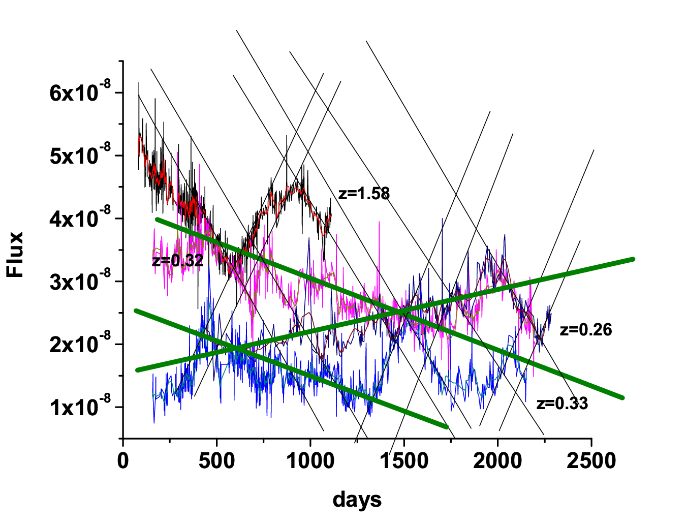

We focus on data with consistent observations over an interval longer than days, since that allows for more reliable identification (or rejection) of the observed patterns. We pick several straight line light curve segments from quasars and shift each segment so that it is centered at the origin (,). If the slope of the segment is negative, we multiply it by , since we are interested only in the absolute value of the slope. We then fit a straight line through the data collected from the corresponding segments of all quasars and find the slope, (see Fig. 2). We assume that all data points have the same weight in order to avoid a single segment giving a dominant contribution. The slope from the least-squares fit is
| (2) |
where the “unit” is . If this pattern of parallel slopes in quasar light curves is not a coincidence, it would indicate that one can use quasars as distance standards, e.g. like Type Ia supernovae.
Finding the redshift of a quasar from its light curve - Linear fit. We now illustrate the procedure of determining the redshift of an unknown quasar from its light curve. We choose a quasar that was not included in our sample of quasars. We identify five segments from its light curve that appear straight and parallel to one another, as shown in Fig. 3 (the number of segments is not crucial – the more the better). We take each of those segments, discarding the rest of the light curve, and shift them so that each segment is centered at (,). Note that the time axis is in observer time, not quasar rest-frame timesince the redshift is “unknown”. We fit the data collected from all the segments (all belonging to the same quasar) with a single straight line and find the slope, as shown in Fig. 4. In this case, the slope is units/day. Comparing this slope with that in Eq. (2) for the quasars rest-frame light curves, we can calculate the redshift of that particular quasar
| (3) |
Indeed, this value is consistent with the known redshift of that quasar, .
The same procedure can be repeated for the slower variations (marked by the thick green lines in Fig. 1). The results are again consistent within the statistical errors, though the error bars on the slope are larger – presumably because of the “noise” from the fast variations as well as from other less coherent variations.


Therefore, if one can identify an oscillation mode that the particular segment of the light curve belongs to, one can readily calculate the redshift from the light curve. Note that this implies that the time dilation (which is simply a counterpart of the redshift) is included in the quasar light curves, in contrast with conclusions in [3] .
Finding the redshift by matching the light curves. Rather than identifying the segments through which we can fit a line as we did above, we could try to match the whole (or significant portions of the) quasar light curves. We do not expect to match the curves from an arbitrary pair of quasars as many different classes of quasars exist. Fig. 5 shows the observed V-band light curves of two quasars of nearly identical redshifts: 206.17052.388 () and 25.3712.72 (). The similarity is not apparent at all. However, for comparison, we can shift the time and flux origin of quasar 25.3712.72 (and flip it):
| (4) |
and are the time and flux after the shifts and flip.


Fig. 6 shows that the shifted light curves overlap with one another remarkably well.
We now define a procedure of finding the redshift of a quasar from its light curve. To do this, we start with the observed quasar light curves, for example 11.8988.1350 () and 5.4892.1971 () We will keep the original data from 11.8988.1350, and manipulate the data from 5.4892.1971 to obtain a match. As in the previous examples, we will use four kinds of global transformations to shift the light curves. The first one is the time shift () which just resets the initial time and has no special physical meaning. The second one is a global offset of the flux intensity (). Our example in Figs. 5 and 6 shows that is also a necessary transformation to allow. Finally, we must rescale the time coordinate by a factor . It is of course this factor that we are most interested in obtaining. Therefore, the complete set of allowed global transformations of the flux is
| (5) |
Applying transformations in Eq. (5) to 5.4892.1971, we can find a very good match with 11.8988.1350, as shown in Fig 7. We also get an approximate value of . Once we have matched the curves, we can identify the region where the light curves have the best overlap. It is that region that we will use to fit the data statistically.

The main goal is to find the value of which gives the best match to the data. From Fig 7, we identify the region where the light curves have the best match (gray area). We extract the light curve data from these regions and transform one of them using , and . We then combine the data from these two light curves into a single light curve, , according to their new time sequence.
To check if a given transformation gives a good match, we fit with a quartic polynomial:
| (6) |
Fig. 8 shows the best fit, for the three-parameter (, and ) fit. We have minimized
| (7) |
with respect to , and . The standard deviation is , where is the total number of data points. Fig. 9 shows in units of as a function of . (We have minimized with respect to and .) Within one (or 68% confidence level) . This is consistent with the actual measured value of .


Conclusions. By studying the data from MACHO quasars behind the Magellanic Clouds [2], we observed patterns in quasar light curves that have previously gone unnoticed. We analyzed the light-curves in two ways. First, we characterized segments of the light curves by the slopes of straight lines through them. These slopes appear to be directly related to the quasars’ redshifts. This allowed us to formulate a method for determining the redshift of an unknown quasar from its light curve. The results match the known values extremely well. This technique appears to allow us to obtain the redshifts of quasars with such linear trends within a few percent. We also formulated an alternative method for determining the redshift that does not rely on a linear fit. Matching the segments of two quasars light curves, we were able to fit for the redshift ratios of the quasars, again within a few percent.
These techniques suggest that similar patterns shared by different quasars may allow them to be used as standard clocks (or candles) to quantify luminosity distance.
We performed our analysis for V-band light curves, though a similar procedure could be carried out for other wavelengths. We currently do not have a theoretical explanation of this effect. We would not want to speculate much on the possible explanation since the physics of these objects is poorly understood. Heuristically, if the frequency, , and the corresponding amplitude, , of the oscillation mode satisfy constant, and one looks at the sine-wave oscillations, then a constant slope would appear for small . Alternatively, it could happen that particular quasi-periodic quasar oscillations described in [7] (see also [8] where similar objects are studied) are behind this effect. For related studies see also [9, 10, 11]. To identify the physics of the pattern we discovered clearly requires further investigation.
Regardless of its theoretical explanation, this observed effect suggests that one might be able to use quasars as distance standards. It will be important to extend the study to other quasars in order to find the dispersion of this effect. This will require a larger sample than the high quality quasar light curves, with continuous coverage over at least days, that are currently available.
Acknowledgements.
This work was partially supported by the US National Science Foundation, under Grants No. PHY-0914893 and PHY-1066278.References
- [1] Baldwin, J.A., et al., Nature, 273, 431 (1978); Baldwin, Jack A., Astrophys. J., 214, 679 (1977); Richstone, D. O., Ratnatunga, K., Schaeffer, J., Astrophys. J., 240, 1 (1980); Mushotzky, R., Ferland, G. J., Astrophys. J., 278, 558 1984 Zamorani, G., et al. MNRAS 256 238 (1992)
- [2] M. Geha et al. [MACHO collaboration], Astron. J. 125, 1 (2003).
- [3] M. R. S. Hawkins, MNRAS, 405, 1940 (2010).
- [4] M. R. S. Hawkins, astro-ph/0105073.
- [5] J. Pelt, et al. A&A, 336, 829 (1998)
- [6] M. Wold, M. S. Brotherton and Z. Shang, MNRAS 375, 989 (2007).
- [7] S. K. Chakrabarti, K. Acharyya and D. Molteni, Astron. Astrophys. 421, 1 (2004) A&A, 421, 1 (2004).
- [8] J. Lovegrove, R. E. Schild and D. Leiter, MNRAS 412 2631 (2011)
- [9] C. L. MacLeod, Z. Ivezic, C. S. Kochanek, S. Kozlowski, B. Kelly, E. Bullock, A. Kimball and B. Sesar et al., Astrophys. J. 721, 1014 (2010) [arXiv:1004.0276 [astro-ph.CO]].
- [10] S. Kozlowski et al. [OGLE Collaboration], Astrophys. J. 708, 927 (2010) [arXiv:0909.1326 [astro-ph.CO]].
- [11] B. C. Kelly, J. Bechtold and A. Siemiginowska, Astrophys. J. 698, 895 (2009) [Erratum-ibid. 732, 128 (2011)] [arXiv:0903.5315 [astro-ph.CO]].