Comparison of Different Parallel Implementaions of the 2+1-Dimensional KPZ Model and the 3-Dimensional KMC Model
Abstract
We show that efficient simulations of the Kardar-Parisi-Zhang interface growth in dimensions and of the -dimensional Kinetic Monte Carlo of thermally activated diffusion can be realized both on GPUs and modern CPUs. In this article we present results of different implementations on GPUs using CUDA and OpenCL and also on CPUs using OpenCL and MPI. We investigate the runtime and scaling behavior on different architectures to find optimal solutions for solving current simulation problems in the field of statistical physics and materials science.
1 Introduction
Statistical physics and materials science use advanced simulation tools to understand complex phenomena prevalent in nature. To analyze the behavior in the thermodynamic limit we need to reach extremely large system sizes and times. Simulations of disordered systems require several hundreds of hours of computing time due to the slow evolution even in one dimension [1].
In present day parallel computing architectures the efficiency of the parallelization is in the focus of software development. Current approaches to write parallel algorithms can be divided into two groups: on one hand thread-parallel algorithms on GPUs (CUDA or OpenCL) and CPUs (OpenCL or OpenMP) and messages-based process-parallel algorithms on the other hand. In applications both concepts can be combined, since threads can only be created on the motherboard, whereas the communication between different units 11 1 different can also mean architectural inhomogeneities can only be realized using message passing.
In this article we investigate two different models, the Kardar-Parisi-Zhang (KPZ) surface growth and the Kinetic Monte Carlo (KMC) of thermally activated diffusion of binary alloys, implemented using different programming models on different architectures. Main specifications of the GPUs used in this work are gathered in Tables 1 and 2, while the most important details of the CPUs utilized for comparison can be found in Table 3. Note, that the performance values in both tables are theoretic.
| NVIDIA C1060 | NVIDIA C2050 / C2070 | |
| (Tesla) | (Fermi) | |
| Number of multiprocessors (mp) | 30 | 14 |
| Number of processing elements | 240 | 448 |
| Clock rate of the mp | 1300 MHz | 1150 MHz |
| Global memory | 4 GB | 2 GB / 6 GB |
| Shared memory per mp | 16 kB | 48 kB2 |
| Memory clock rate | 800 MHz | 1500 MHz |
| Global memory bandwidth | 102 GB/s | 144 GB/s |
| Peak performance (single precision) | 936 GFlop/s | 1030 GFlop/s |
| Peak performance (double precision) | 78 GFlop/s | 515 GFlop/s |
| ATI Radeon HD5970 | ATI Radeon HD6970 | |
| Number of multiprocessors (mp) | 40 | 24 |
| Number of processing elements | 3200 | 1536 |
| Clock rate of the mp | 725 MHz | 880 MHz |
| Global memory | 2 GB | 2 GB |
| Shared memory per mp | 32 kB | 32 kB |
| Memory clock rate | 1000 MHz | 1375 MHz |
| Global memory bandwidth | 256 GB/s | 256 GB/s |
| Peak performance (single precision) | 4640 GFlop/s | 2703 GFlop/s |
| Peak performance (double precision) | 928 GFlop/s | 675 GFlop/s |
| AMD Opteron | Intel Core i5 | Intel Core i7 | |
|---|---|---|---|
| F8380 | 430 M | 920 | |
| Number of cores | 4 | 2 | 4 |
| Clock rate | 2500 MHz | 2267 MHz | 2664 MHz |
| L1 cache | 4 128 kB | 2 64 kB | 4 64 kB |
| L2 cache | 4 512 kB | 2 256 kB | 4 256 kB |
| L3 cache | 6 MB | 3 MB | 8 MB |
| Peak performance | 49,16 GFlop/s | 39,68 GFlop/s | 88,97 GFlop/s |
In Section 2 we present the two models used in this work: the KPZ growth and the KMC method of binary alloys. Details about the implementation of these two models are presented in Section 3. In Section 4 we show the efficiency results of the different implementations and we conclude with Section 5.
2 Overview of the models
2.1 The Kardar-Parisi-Zhang model
The Kardar-Parisi-Zhang (KPZ) equation was inspired in part by the the stochastic Burgers equation [2], which belongs to the same universality class [3] and it became the subject of many theoretical studies [5, 4, 6]. Besides, it models other important physical phenomena such as directed polymers [7], randomly stirred fluid [3], dissipative transport [9, 8] and the magnetic flux lines in superconductors [10]. Due to the mapping onto the Asymmetric Exclusion Process (ASEP) [12] it is also a fundamental model of a non-equilibrium particle system [13], with broken detailed balance condition
| (1) |
where denotes the probability of the state and is the transition rate between states and .
The KPZ equation specifies the evolution of the height function in the dimensional space
| (2) |
Here and are the amplitudes of the mean and local growth velocity, is a smoothing surface tension coefficient and roughens the surface by a zero-average, Gaussian noise field exhibiting the variance
| (3) |
The letter denotes the noise amplitude and means distribution average. The equation is solvable in due to the Galilean symmetry 33 3 The invariance of Eq. (2) under an infinitesimal tilting of the interface, [3] and an incidental fluctuation-dissipation symmetry [11], while in higher dimensions approximations are available only. The model exhibits diverging correlation length, hence a scale invariance, that can be understood by the particle current in the ASEP model. The current corresponds to the up-down anisotropy of the KPZ. Therefore KPZ equation has been investigated by renormalization techniques [14, 15, 16]. The KPZ phase space has been the subject of controversies for a long time [19, 20] and the strong coupling fixed point has been located by non-perturbative RG very recently [21]. Values of the surface scaling exponents for exhibit considerable uncertainties (see [4]), we provided very high precision simulation results in [24, 29].
Discretized versions of KPZ have also been studied a lot ([18, 19, 22], for a review see [4]). Recently we have shown [23, 24] that the mapping between a restricted solid on solid representation of the KPZ surface growth and the ASEP [25, 26] can straightforwardly be extended to higher dimensions. In 2+1 dimensions the mapping is just the simple extension of the rooftop model to the octahedron model as can be seen on Figure 2 of [23]. The surface built up from the octahedra can be described by the edges meeting in the up/down middle vertexes. Up edges in the or directions are approximated by the derivatives , while the down ones by . Note, that in a renormalizable system, such as the KPZ different slopes without overhangs can approximated on this way. This can also be understood as a special cellular automaton [27] with the generalized Kawasaki updating rules
| (4) |
with probability for attachment and probability for detachment. We have confirmed that this mapping, using the parametrization: , reproduces the one-point functions of the continuum model. This kind of generalization of the ASEP model can be regarded as the simplest candidate for studying KPZ in : a one-dimensional model of self-reconstructing -mers [28] diffusing in the -dimensional space. Furthermore this lattice gas can be studied by very efficient simulation methods.
We followed the evolution of the lattice gases of linear size (), started from flat initial configuration. Periodic boundary conditions are applied. The surface heights (see Fig. 1) are reconstructed from the slopes
| (5) |
and the squared interface width
| (6) |
was calculated at certain sampling times ().

The results are written out during the run to the disk and analyzed later by statistical methods as discussed in [29].
2.2 Kinetic Monte Carlo
The Kinetic Monte Carlo (KMC) Method models atomistic on-lattice dynamics on large spatio-temporal scales [33]. Commonly atomistic simulations are performed by solving Hamilton equations for a system (i. e. Molecular Dynamics). The general idea of KMC is to use a thermodynamic model to average out microscopic fluctuations, creating a probabilistic model of on-lattice particle movement. This model has been successfully applied to a variety of phenomena of self-organization, for Ostwald ripening, investigations of the Plateau Rayleigh instability [31] and phenomena in systems driven by ion bombardment, like the creation of surface ripples [32] and inverse Ostwald ripening [30]. Our GPU implementation puts simulations at experimental spatio-temporal scales within reach.
Kinetic Lattice Monte Carlo employs a totalistic stochastic probabilistic cellular automaton [38], in the present case based on the nearest neighbor Ising model with Kawasaki dynamics [36]. System evolution based, for example, on the interatomic many-body RGL potential [48] can be treated too. In this work we will focus on the case of a binary alloy containing two species A and B, encoded as single bits and , respectively. To make the model valid for most metals and to get a good approximation for amorphous materials a face centered cubic simulation lattice is used [34], where each particle has twelve nearest neighbors. The simulation lattice is stored as a sub-lattice of a simple cubic lattice [33], where valid fcc coordinates are identified by
| (7) |
where denotes the logic bit-wise XOR.
The cellular automaton follows the Metropolis algorithm [37], where species B is regarded active, while species A provides a surrounding matrix which is passive. The role of species A and B can easily be exchanged by a particle–hole transformation of the Hamiltonian. Through the course of the simulations update attempts are called one Monte Carlo Step (MCS) in a lattice containing sites. The simulation time is measured in this unit, which only gains physical meaning for large times [33].
In an update attempt [31] a random lattice site is chosen. If the chosen initial site is not occupied by a specimen of B the attempt is finished, otherwise a random nearest neighbor is chosen as the final site . If site is occupied by the other species the content of sites is exchanged according to the Metropolis transition probability
| (8) |
where and are the numbers of nearest neighbor sites of and , respectively, occupied with atoms of species B, is an effective jump frequency, incorporating an activation energy barrier for the transition and is the effective temperature. In our present work we set
| (9) |
3 Implementation of the Models
When we parallelize a stochastic cellular automaton algorithm, to which both models discussed here resemble, the basic idea is to find a way of performing multiple updates independently. The main task is to generate a Markov chain of states, requiring site updates to be statistically independent. This can be achieved by domain decomposition: the system is divided into sets of non-interacting domains. Each domain of a set is assigned to a worker temporarily, while other sets remain inactive. The simplest decomposition scheme is the checkerboard decomposition [41], but we have chosen different methods.
Dead border decomposition is a scheme that has already been successfully employed for KPZ [29]. The system is decomposed into blocks, updated independently leaving out their border. After some time the origin of the decomposition is moved randomly to allow changes in the individual cells to propagate through the whole lattice (see Fig. 2a).


Another scheme, more suitable when well aligned memory accesses are important, is the double tiling method. The system is decomposed into tiles, bisected in each direction, creating sets of independent domains. These sets are updated in turn, generally by a randomized sequence, and each domain of the currently active set is assigned to a different worker (Fig. 2b). This approach was also used in [46] for a two dimensional multi-CPU implementation of different variation of KMC.
By employing domain decomposition one deviates from the original model. This leads to errors at domain boundaries, which cannot be eliminated completely, but one must keep them sufficiently small. When a cell is updated it temporarily becomes a separate system with fixed boundary conditions determined by the neighbors. For sufficiently small times, this is a good approximation to a part of a system continuously interacting with the surroundings.
We used domain decomposition at each layer of the parallelization independently. On a single GPU there are two layers to be taken into account. The device layer, where the system has to distributed over the compute units (work-groups in OpenCL terminology, thread block in CUDA) and the work-group layer, where the cell assigned to a work-group is distributed among the threads (or work-items in OpenCL). See [42] for a overview of GPU architecture.
3.1 The dimensional KPZ algorithm
We implemented the dimensional KPZ both using CUDA and OpenCL. Our analysis was restricted to the , case, while the code could easily handle more general conditions. An earlier version of our CUDA implementation was presented in [29], where dead border decomposition was applied at both layers. Here we improve that application by employing a more efficient, single–hit double tiling scheme at the work-group layer, while the device layer remains unchanged. Because the problem is two dimensional there are sets of, quite small, non-interacting cells. Performing full updates here, i. e. giving all sites of the cell the chance to be updated once before moving on the next cell, would allow the effects of fixing neighboring cells to become significant. Under these conditions the aforementioned approximation of temporarily treating the cell as a system with fixed boundaries would become bad. Single–hit means, that a cell receives only a single update attempt before the work-group, i. e. the threads collectively, move on to another random set of cells (it may be the same set). Single–hits repeated until, on average, each site of the work-group’s block had the chance to be updated once. Performing single–hit updates effectively eliminates errors at domain boundaries, only leaving simultaneous updates slightly correlated.
This implementation was straightforwardly ported to OpenCL, showing almost no difference in performance on NVIDA Tesla C2070 cards. It is however optimized for NVIDA’s architectures and thus cannot make optimal use of AMD devices. The main difference between the two architectures, connected to our applications is that NVIDIA provides 32–bit scalar registers, while AMD uses 128–bit registers build for vector operations. AMD devices can only be fully utilized by issuing operations on vectors of four 32–bit values. AMD devices allow different instructions for different vector components, a technology called very long instruction word (VLIW). The compiler may use this by automatically vectorizing code that contains independent operations. Our CUDA implementation does not use vector operations and leaves no room for auto vectorization, thus it can only utilize such a device to a quarter.
We created an OpenCL implementation optimized for AMD devices vectorizing the code by hand. The basic approach was to utilize the vector capabilities of the device by executing a virtual thread in each vector component. At device layer dead border decomposition is employed. At work-group layer a worker is identical to a virtual thread. There double tiling is used to distribute the work-group’s chunk among all virtual threads. (Fig. 3)
As in the CUDA implementation the work-group layer updates are single–hit. The difference is, that each work-item is assigned four domains of the collectively chosen set. These four update are then carried out using vector operations, thus achieving a maximum utilization of the ALU.
For random number generation we used different algorithms: 32-bit linear congruential (LCRNG), skip-ahead 64-bit LCRNG [42] and Mersenne Twister [43]. Comparing them by very extensive KPZ simulations (several weeks of test runs) have shown no noticeable differences in the scaling results [29]. Our OpenCL implementation employs a special version of the Mersenne Twister called TinyMT [44] for random number generation.

3.2 Implementation of KMC
The GPU implementation of KMC employs a two-layer double tiling domain decomposition scheme tailored to the two-layered computing architecture of GPUs. At device layer the system is tiled, each tile consisting of eight blocks (). Subsets of the blocks are fully updated in a sequence randomized at each MCS, where each block of the current set is assigned to a work-group. For performance reasons the system size is restricted to powers of two, leading to a number of blocks which itself is a power of two. However, the number of multiprocessors on available GPUs is not a power of two. To compensate for that (to maximize utilization), part of the super blocks are updated ahead of time.44 4 This does not introduce an error since the unit MCS only has physical meaning in the limit of large times, where time ordering is broken at the scale of two MCS. At work-group layer the same decomposition scheme as of the optimized KPZ implementation is used:55 5 Actually KPZ inherited this scheme from KMC. double checkerboard with single hit updates.
On the GPU all threads of a block have to be synchronized, so there is no benefit from earlier termination of a thread, this would just leave part of the device idle. Since this happens frequently if only one species is considered to be active (see Section 2.2), both species are considered to be active in the GPU code. Equation (8) can still be used for this, only the roles of the initial and final sites are reversed if is occupied by A. The CUDA implementation was directly ported to OpenCL, as for the KPZ CUDA implementation almost no difference in performance has been found on a C2070.
The condition of detailed balance [47] is satisfied locally up to the work-group layer. When stepping through the domain sets at device level, detailed balance is broken for the last few updates performed within the individual cells, because they cannot be reversed instantly. In any way this effect is too small to give rise any measurable effect, small disturbances of kinetics directly at domain boundaries are of far greater concern [35].
The CPU MPI implementation of KMC uses dead border decomposition scheme in one dimension. This reduces the communication overhead by improving the surface to bulk ratio of cells, which limits the communication of each node to its neighbors. The downside of this method is a lower number of workers that can be used for fixed system size as compared to a method with decomposition along more dimensions. There is a lower limit for lateral chunk sizes one cannot go below without hurting the statistics.
Benchmarks comparing GPU and CPU implementations exposed a problem with the CPU implementations when dealing with very large systems for both KMC and KPZ. Since sites to be updated are chosen randomly the CPU can only make use of it’s caches as long as the whole system fits at least in the last level cache.66 6 For Intel CPU’s last level means L3, for AMD L2. If the system size exceeds the cache size the cache becomes effectively useless, causing a significant drop in the CPU performance. [29]
This can be avoided by decomposing the system into blocks, which are updated randomly. The largest performance gain can be achieved when those blocks are not larger that half of the size of the L1 cache. This can also be done in an MPI implementation. The benefit is less in smaller systems, respectively smaller domains, for an already parallel implementation.
4 Run-time comparison
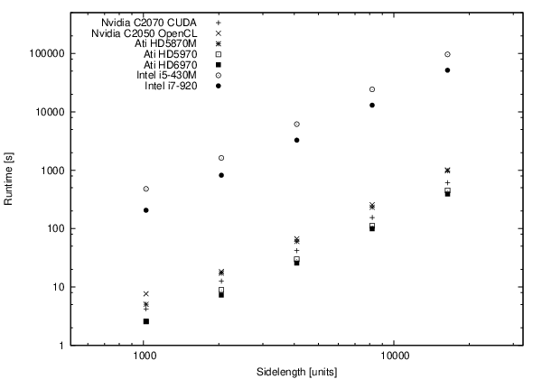
We implemented different versions of the KPZ and KMC models using CUDA, OpenCL and MPI for the different platforms mentioned in Tables 1, 2 and 3. In Figure 4 we collected the run-times of a given task measured on different implementations. It is easy to see that the execution on GPUs is up to two orders of magnitude faster than on CPUs. Moreover it is not surprising that the mobility versions of CPUs and GPUs exhibit lower performances.
The number of domains the system is decomposed into is not a multiple of the number of compute units. Say the system is decomposed into domains and the device provides compute units (see tables 1 and 2), with and . The device is completely utilized for a fraction
of time, during the remaining time only compute units are busy. An increasing with leads to a sub-linear scaling of runtime with the system size. In KMC we avoid this problem trough the aforementioned block-ahead of time updating method, which is not possible using dead border decomposition.
In order to give a more illustrative idea on the performance differences between CPU and GPU codes, Figure 5 shows the number of updates per second on different architectures used. This value is a more practical one, because it really expresses the speed of a real physics application.

To benchmark our implementations of lattice KMC we simulated the quenching process of a system with an fcc lattice of sites. We started from a homogeneous mixture with concentration of species and effective temperature . Under these conditions spinodal decomposition is observed. To provide some significance regarding real world applications at least were performed. Since the workload changes as phase separation and subsequent coarsening take place: The number of successful update attempts decreases. Figure 6 lists some of our results. The performance was normalized to the fastest single CPU implantation at hand. The cache optimized version (CPU DD) was almost five times faster than the classical CPU implementation on the AMD Opteron CPU used.
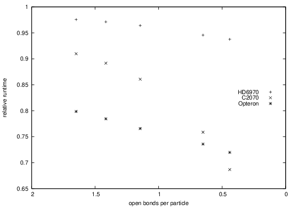
The straightforward OpenCL port of our CUDA implementation exhibits almost the same performance on the same device, but it cannot utilize an HD6970 completely. We also noted another difference between NVIDIA and AMD devices. As the warp size on NVIDIA devices is smaller than on AMD devices, the C2070 can profit better from an increased rate of failing update attempts than the HD6970. In fact, the HD6970 turned out to be slightly faster than a C2070 for short runs, when almost all update attempts were successful. Figure 7 shows timing of short runs at late stages of the evolution relative times measured at the initial state.

Our MPI implementation reaches an efficiency of for large numbers of CPUs spread over multiple nodes. Because the system is only decomposed in one direction no more that 32 cores can be used for a system of the given size/aspect ratio. When all CPUs are located on a single node an efficiency of is reached. In this case cache optimization was used.
Although it is possible to run OpenCL code on CPUs, it is not really efficient with our application. Our tests show that OpenCL cannot keep its promise to enable architecture independent parallel computing. Our code, designed for NVIDIA GPUs, performs very badly on CPUs. Using 16 cores it delivers results only two times faster than a single core using cache optimization.
5 Conclusions and outlook
We have implemented and compared different GPU and CPU realizations using CUDA, OpelCL and MPI for two applications: the d KPZ surface growth and phase separation of a binary, immiscible mixture in a 3d lattice KMC system. We used dead border [29] and double tiling domain decomposition, the latter turned out to be more efficient. According to the benchmarks OpenCl performs almost as good as CUDA on NVIDIA devices, but it could not fulfill it’s promise on platform independence. Using KPZ as an example we have shown, that adjusting the code to platform specifics has a large impact on performance and optimizing for one platform may result in performance penalties on the another. Our AMD-optimized OpenCl implementation of KPZ is considerably slower on NVIDIA GPUs than the straightforward port from CUDA. The same is true for running OpenCL code designed for GPUs on a CPU. Our MPI implementation of KMC outperforms our OpenCL implementation on CPUs. Parallelizations of these applications by MPI on CPU clusters up to 32 cores show low efficiency.
The cellular automaton approach in GPU simulations has been shown to be very efficient, because it allows bit coding as well as massively parallel computing. This enabled us to simulate Ising type of models on unprecedentedly large scales both in space and time. In particular we could study KPZ surface growth on sizes up to lattice sites and a speedup was measured on Fermi cards with respect to an I5-750 CPU core. For KMC a speedup of was found with respect to a Xeon E5530 core. We assume the lower speedup was due to the higher spatial dimension rather than the complexity of KMC with respect to KPZ. As we increase , the number of lattice sites a work-item must occupy grows. Since the local memory is limited, this decrases the number of work-items that can be run per block. Furthermore, mapping of a higher dimensional system onto a linear array, the locality of memory accesses decreases, increasing the possibility of bank conflicts on GPUs. For systems of equal volume, the latter should have no effect when running on CPUs, as long as the system, respectively subsystem, fits into the cache. The statistical analysis of the results has been presented elsewhere [29].
This kind of surface mapping can be extended by other competing processes, resulting in surface patterns. In particular, ripple and dot formation has been studied in [39, 40]. Implementation on GPUs can lead to fast simulation of larger systems, which is essential in case of the slow surface diffusion, quenched disorder [1], or by performing aging studies [45].
6 Acknowledgments
We thank Nils Schmeißer for the useful discussions on parallelizing KMC using MPI. Support from the Hungarian research fund OTKA (Grant No. T77629), OSIRIS FP7 and the bilateral German-Hungarian exchange program DAAD-MÖB (Grant Nos. 50450744, P-MÖB/854) is acknowledged. The authors thank NVIDIA for supporting the project with high-performance graphics cards within the framework of Professor Partnership.
References
- (1) H. Schulz, Gergely Ódor, Géza Ódor, and Máté Ferenc Nagy, Comp. Phys. Comm. 182, (2011) 1467.
- (2) J. M.Burgers, The Nonlinear Diffusion Equation, (Riedel, Boston 1974).
- (3) D. Forster, Phys. Rev. A, 16, (1977) 732.
- (4) A. L. Barabási and H. E. Stanley, Fractal Concepts in Surface Growth, (Cambridge University Press, Cambridge 1995).
- (5) T. Halpin-Healy and Y.-C. Zhang, Phys. Rep. 254, (1995) 215.
- (6) J. Krug, Adv. Phys. 46, (1997) 139.
- (7) M. Kardar, Phys. Rev. Lett. 55, (1985) 2923
- (8) H. K. Janssen and B. Schmittmann, Z. Phys. B, 63, (1986) 517.
- (9) H. van Beijeren, R. Kutner and H. Spohn, Phys. Rev. Lett. 54, (1985) 2056.
- (10) T. Hwa, Phys. Rev. Lett. 69, (1992) 1552.
- (11) M. Kardar, Nucl. Phys. B 290, (1987) 582.
- (12) H. Rost, Z. Wahrsch. Verw. Gebiete, 58, (1981) 41.
- (13) G. Ódor, Universality In Nonequilibrium Lattice Systems, (World Scientific 2008).
- (14) M. Schwartz and S.F. Edwards, Europhys. Lett. 20, (1992) 301.
- (15) E. Frey and U. C. Täuber, Phys. Rev. E, 50, (1994) 1024.
- (16) M. Lässig, Nucl. Phys. B, 448 (1995) 559.
- (17) B. M. Forrest and L. H. Tang, Phys. Rev. Lett, 64, (1990) 1405.
- (18) E. Marinari, A. Pagnani and G. Parisi, J. Phys. A 33, (2000) 8181.
- (19) E. Marinari, A. Pagnani, G. Parisi and Z. Rácz, Phys. Rev. E 65 (2002) 026136.
- (20) H. C. Fogedby, Phys. Rev. Lett. 94, (2005) 195702.
- (21) L. Canet, H. Chaté, B. Delamotte, N. Wschebor, Phys. Rev. E 84 (2011) 061128.
- (22) F. D. A AaraoReis, Phys. Rev. E 72 (2005) 0322601.
- (23) G. Ódor, B. Liedke and K.-H.Heinig, Phys. Rev. E 79, (2009) 021125.
- (24) G. Ódor, B. Liedke and K.-H.Heinig, Phys. Rev. E 81, (2010) 031112.
- (25) M. Plischke, Z. Rácz and D. Liu, Phys. Rev. B 35, (1987) 3485.
- (26) P. Meakin, P. Ramanlal, L. M. Sander and R. C. Ball, Phys. Rev. A 34, (1986) 5091.
- (27) S. Wolfram, Rev. Mod. Phys. 55, (1983) 601.
- (28) M. Barma, M. D. Grynberg and R. B. Stinchcombe, J. Phys.: Condens. Matter 19, (2007) 065112.
- (29) J. Kelling and G. Ódor, Phys. Rev. E 84, (2011) 061150.
- (30) K.-H. Heinig, T. Müller, B. Schmidt, M. Strobel and W. Möller, Appl. Phys. A 77, (2003) 17
- (31) L. Röntzsch, Phd Thesis, (2007)
- (32) B. Liedke, Phd Thesis, (2011)
- (33) M. Strobel, Phd Thesis, (1999)
- (34) T. Müller, Phd Thesis, (2005)
- (35) J. Kelling, Diploma Thesis, (2012)
- (36) K. Kawasaki, Phys. Rev. 145, (1966) 224
- (37) N. Metropolis et al., J. of Chem. Phys. 21 (1953) 1087¿1092.
- (38) S. Wolfram, A new kind of science, (2002)
- (39) G. Ódor, B. Liedke and K.-H. Heinig, Phys. Rev. E 81, 051114 (2010).
- (40) G. Ódor, B. Liedke, K.-H. Heinig and J. Kelling, Appl. Surf. Sci. 258 (2012) 4186-4190.
- (41) T. Preis et al. GPU accelerated Monte Carlo simulation of the 2D and 3D Isingmodel. J. Comp. Phys. 228:4468-4477, 2009.
- (42) M. Weigel. Performance potential for simulating spin models on GPU. J. Comput. Phys., 231 (2012) 3064.
- (43) M. Matsumoto, et al., J. of. Univ. Comp. Sci. 12 (2006) 672.
- (44) TinyMT website http://www.math.sci.hiroshima-u.ac.jp/ m-mat/MT/TINYMT/index.html
- (45) M. Henkel, J. D. Noh and M. Pleimling, Phys. Rev. E 85 (2012) 030102(R)
- (46) Shim, Y., Amar, J.G., Phys. Rev. B 71(12), APS, 125432, 2005
- (47) Newman, M. E. J., Barkema, G. T. Monte Carlo Methods in Statistical Physics, Oxford University Press, 1999
- (48) V. Rosato, M. Guillope, B. Legrand, Phil. Mag. A 59(2), 321-336 (1989)