Branch Flow Model: Relaxations and Convexification (Part I) Thanks: To appear in IEEE Trans. Power Systems, 2013 (submitted in May 11, 2012, accepted for publication on March 3, 2013). A preliminary and abridged version has appeared in [1].

The bus injection model is the standard model for power flow analysis and optimization. It focuses on nodal variables such as voltages, current and power injections and does not directly deal with power flows on individual branches. Instead of nodal variables, the branch flow model focuses on currents and powers on the branches. It has been used mainly for modeling distribution circuits which tend to be radial, but has received far less attention. In this paper, we advocate the use of branch flow model for both radial and mesh networks, and demonstrate how it can be used for optimizing the design and operation of power systems.

One of the motivations for our work is the optimal power flow (OPF) problem. OPF seeks to optimize a certain objective function, such as power loss, generation cost and/or user utilities, subject to Kirchhoff’s laws, power balance as well as capacity, stability and contingency constraints on the voltages and power flows. There has been a great deal of research on OPF since Carpentier’s first formulation in 1962 [2]; surveys can be found in, e.g., [3, 4, 5, 6, 7]. OPF is generally nonconvex and NP-hard, and a large number of optimization algorithms and relaxations have been proposed. A popular approximation is the DC power flow problem, which is a linearization and therefore easy to solve, e.g. [8, 9, 10, 11]. An important observation was made in [12, 13] that the full AC OPF can be formulated as a quadratically constrained quadratic program and therefore can be approximated by a semidefinite program. While this approach is illustrated in [12, 13] on several IEEE test systems using an interior-point method, whether or when the semidefinite relaxation will turn out to be exact is not studied. Instead of solving the OPF problem directly, [14] proposes to solve its convex Lagrangian dual problem and gives a sufficient condition that must be satisfied by a dual solution for an optimal OPF solution to be recoverable. This result is extended in [15] to include other variables and constraints and in [16] to exploit network sparsity. In [17, 18], it is proved that the sufficient condition of [14] always holds for a radial (tree) network, provided the bounds on the power flows satisfy a simple pattern. See also [19] for a generalization. These results confirm that radial networks are computationally much simpler. This is important as most distribution systems are radial.

The limitation of semidefinite relaxation for OPF is studied in [20] using mesh networks with 3, 5, and 7 buses: as a line-flow constraint is tightened, the duality gap becomes nonzero and the solutions produced by the semidefinite relaxation becomes physically meaningless. Indeed, examples of nonconvexity have long been discussed in the literature, e.g., [21, 22, 23]. See, e.g., [24] for branch-and-bound algorithms for solving OPF when convex relaxation fails.

The papers above are all based on the bus injection model. In this paper, we introduce a branch flow model on which OPF and its relaxations can also be defined. Our model is motivated by a model first proposed by Baran and Wu in [25, 26] for the optimal placement and sizing of switched capacitors in distribution circuits for Volt/VAR control. One of the insights we highlight here is that the Baran-Wu model of [25, 26] can be treated as a particular relaxation of our branch flow model where the phase angles of the voltages and currents are ignored. By recasting their model as a set of linear and quadratic equality constraints, [27, 28] observe that relaxing the quadratic equality constraints to inequality constraints yields a second-order cone program (SOCP). It proves that the SOCP relaxation is exact for radial networks, when there are no upper bounds on the loads. This result is extended here to mesh networks with line limits, and convex, as opposed to linear, objective functions (Theorem 1). See also [29, 30] for various convex relaxations of approximations of the Baran-Wu model for radial networks.

Other branch flow models have also been studied, e.g., in [31, 32, 33], all for radial networks. Indeed [31] studies a similar model to that in [25, 26], using receiving-end branch powers as variables instead of sending-end branch powers as in [25, 26]. Both [32] and [33] eliminate voltage angles by defining real and imaginary parts of $V_{i}V_{j}^{*}$ as new variables and defining bus power injections in terms of these new variables. This results in a system of linear quadratic equations in power injections and the new variables. While [32] develops a Newton-Raphson algorithm to solve the bus power injections, [33] solves for the branch flows through an SOCP relaxation for radial networks, though no proof of optimality is provided.

This set of papers [25, 26, 31, 32, 33, 29, 27, 30, 28] all exploit the fact that power flows can be specified by a simple set of linear and quadratic equalities if voltage angles can be eliminated. Phase angles can be relaxed only for radial networks and generally not for mesh networks, as [34] points out for their branch flow model, because cycles in a mesh network impose nonconvex constraints on the optimization variables (similar to the angle recovery condition in our model; see Theorem 2 below). For mesh networks, [34] proposes a sequence of SOCP where the nononvex constraints are replaced by their linear approximations and demonstrates the effectiveness of this approach using seven network examples. In this paper we extend the Baran-Wu model from radial to mesh networks and use it to develop a solution strategy for OPF.

Our purpose is to develop a formal theory of branch flow model for the analysis and optimization of mesh as well as radial networks. As an illustration, we formulate OPF within this alternative model, propose relaxations, characterize when a relaxed solution is exact, prove that our relaxations are always exact for radial networks when there are no upper bounds on loads but may not be exact for mesh networks, and show how to use phase shifters to convexify a mesh network so that a relaxed solution is always optimal for the convexified network.

Specifically we formulate in Section II the OPF problem using branch flow equations involving complex bus voltages and complex branch current and power flows.

In Section III we describe our solution approach that consists of two relaxation steps (see Figure 1):

• •

  Angle relaxation: relax OPF by eliminating voltage and current angles from the branch flow equations. This yields the (extended) Baran-Wu model and a relaxed problem OPF-ar which is still nonconvex due to a quadratic equality constraint.

• •

  Conic relaxation: relax OPF-ar by changing the quadratic equality into an inequality constraint. This yields a convex problem OPF-cr (which is an SOCP when the objective function is linear).

In Section IV we prove that the conic relaxation OPF-cr is always exact even for mesh networks, provided there are no upper bounds on real and reactive loads, i.e., any optimal solution of OPF-cr is also optimal for OPF-ar. Given an optimal solution of OPF-ar, whether we can derive an optimal solution of the original OPF depends on whether we can recover the voltage and current angles from the given OPF-ar solution. In Section V we characterize the exact condition (the angle recovery condition) under which this is possible, and present two angle recovery algorithms. The angle recovery condition has a simple interpretation: any solution of OPF-ar implies an angle difference across a line, and the condition says that the implied angle differences sum to zero (mod $2\pi$) around each cycle. For a radial network, this condition holds trivially and hence solving the conic relaxation OPF-cr always produces an optimal solution for OPF. For a mesh network, the angle recovery condition corresponds to the requirement that the implied phase angle differences sum to zero around every loop. The given OPF-ar solution may not satisfy this condition, but our characterization can be used to check if it yields an optimal solution for OPF. These results suggest an algorithm for solving OPF as summarized in Figure 2.

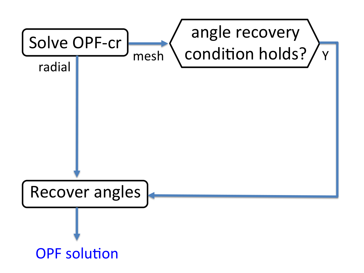
If a relaxed solution for a mesh network does not satisfy the angle recovery condition, then it is infeasible for OPF. In Part II of this paper, we propose a simple way to convexify a mesh network using phase shifters so that any relaxed solution of OPF-ar can be mapped to an optimal solution of OPF for the convexified network, with an optimal cost that is lower than or equal to that of the original network.

In [35, 36], we prove a variety of sufficient conditions under which the conic relaxation proposed here is exact for radial networks. The main difference from Theorem 1 below is that, [35, 36] allow upper bounds on the loads but relax upper bounds on voltage magnitudes. Unlike the proof for Theorem 1 here, those in [35, 36] exploit the duality theory.

The bus injection model and the branch flow model are defined by different sets of equations in terms of their own variables. Each model is self-contained: one can formulate and analyze power flow problems within each model, using only nodal variables or only branch variables. Both models (i.e., the sets of equations in their respective variables), however, are descriptions of the Kirchhoff’s laws. In [37] we prove formally the equivalence of these models, in the sense that given a power flow solution in one model, one can derive a corresponding power flow solution in the other model. Although the semidefinite relaxation in the bus injection model is very different from the convex relaxation proposed here, [37] also establishes the precise relationship between the various relaxations in these two models. This is useful because some results are easier to formulate and prove in one model than in the other. For instance, it is hard to see how the upper bounds on voltage magnitudes and the technical conditions on the line impedances in [35, 36] for exactness in the branch flow model affect the rank of the semidefinite matrix variable in the bus injection model, although [37] clarifies conditions that guarantee their equivalence.

Let $G=(N,E)$ be a connected graph representing a power network, where each node in $N$ represents a bus and each link in $E$ represents a line (condition A1). We index the nodes by $i=0,1,\dots,n$. The power network is called radial if its graph $G$ is a tree. For a distribution network, which is typically radial, the root of the tree (node 0) represents the substation bus. For a (generally meshed) transmission network, node 0 represents the slack bus.

We regard $G$ as a directed graph and adopt the following orientation for convenience (only). Pick any spanning tree $T:=(N,E_{T})$ of $G$ rooted at node 0, i.e., $T$ is connected and $E_{T}\subseteq E$ has $n$ links. All links in $E_{T}$ point away from the root. For any link in $E\setminus E_{T}$ that is not in the spanning tree $T$, pick an arbitrary direction. Denote a link by $(i,j)$ or $i\rightarrow j$ if it points from node $i$ to node $j$. Henceforth we will assume without loss of generality that $G$ and $T$ are directed graphs as described above.¹¹ 1 The orientation of $G$ and $T$ are different for different spanning trees $T$, but we often ignore this subtlety in this paper. For each link $(i,j)\in E$, let $z_{ij}=r_{ij}+\textbf{i}x_{ij}$ be the complex impedance on the line, and $y_{ij}:=1/z_{ij}=:g_{ij}-\textbf{i}b_{ij}$ be the corresponding admittance. For each node $i\in N$, let $z_{i}=r_{i}+\textbf{i}x_{i}$ be the shunt impedance from $i$ to ground, and $y_{i}:=1/z_{i}=:g_{i}-\textbf{i}b_{i}$.²² 2 The shunt admittance $y_{i}$ represents capacitive devices on bus $i$ only and a line is modeled by a series admittance $y_{ij}$ without shunt elements. If a shunt admittance $\textbf{i}\tilde{b}_{ij}/2$ is included on each end of line $(i,j)$ in the $\pi$-model, then a limit on line flow should be a limit on $\left|S_{ij}-\textbf{i}\tilde{b}_{ij}|V_{i}|^{2}/2\right|$ instead of on $|S_{ij}|$.

For each $(i,j)\in E$, let $I_{ij}$ be the complex current from buses $i$ to $j$ and $S_{ij}=P_{ij}+\textbf{i}Q_{ij}$ be the sending-end complex power from buses $i$ to $j$. For each node $i\in N$, let $V_{i}$ be the complex voltage on bus $i$. Let $s_{i}$ be the net complex power injection, which is generation minus load on bus $i$. We use $s_{i}$ to denote both the complex number $p_{i}+\textbf{i}q_{i}$ and the pair $(p_{i},q_{i})$ depending on the context.

As customary, we assume that the complex voltage $V_{0}$ is given and the complex net generation $s_{0}$ is a variable. For power flow analysis, we assume other power injections $s:=(s_{i},i=1,\dots,n)$ are given. For optimal power flow, VAR control, or demand response, $s$ are control variables as well.

Given $z:=(z_{ij},(i,j)\in E,\ z_{i},i\in N)$, $V_{0}$ and bus power injections $s$, the variables $(S,I,V,s_{0}):=(S_{ij},I_{ij},(i,j)\in E,\ V_{i},i=1,\dots,n,\ s_{0})$ satisfy the Ohm’s law:

the definition of branch power flow:

and power balance at each bus: for all $j\in N$,

We will refer to (1)–(3) as the branch flow model/equations. Recall that the cardinality $|N|=n+1$ and let $|E|=:m$. The branch flow equations (1)–(3) specify $2m+n+1$ nonlinear equations in $2m+n+1$ complex variables $(S,I,V,s_{0})$, when other bus power injections $s$ are specified.

We will call a solution of (1)–(3) a branch flow solution with respect to a given $s$, and denote it by $x(s):=(S,I,V,s_{0})$. Let $\mathbb{X}(s)\subseteq\mathbb{C}^{2m+n+1}$ be the set of all branch flow solutions with respect to a given $s$:

and let $\mathbb{X}$ be the set of all branch flow solutions:

For simplicity of exposition, we will often abuse notation and use $\mathbb{X}$ to denote either the set defined in () or that in (5), depending on the context. For instance, $\mathbb{X}$ is used to denote the set in () for a fixed $s$ in Section V for power flow analysis, and to denote the set in (5) in Section IV for optimal power flow where $s$ itself is also an optimization variable. Similarly for other variables such as $x$ for $x(s)$.

Consider the optimal power flow problem where, in addition to $(S,I,V,s_{0})$, $s$ is also an optimization variable. Let $p_{i}:=p_{i}^{g}-p_{i}^{c}$ and $q_{i}:=q_{i}^{g}-q_{i}^{c}$ where $p_{i}^{g}$ and $q_{i}^{g}$ ($p_{i}^{c}$ and $q_{i}^{c}$) are the real and reactive power generation (consumption) at node $i$. For instance, [25, 26] formulate a Volt/VAR control problem for a distribution circuit where $q_{i}^{g}$ represent the placement and sizing of shunt capacitors. In addition to (1)–(3), we impose the following constraints on power generation: for $i\in N$,

In particular, any of $p_{i}^{g},q_{i}^{g}$ can be a fixed constant by specifying that $\underline{p}_{i}^{g}=\overline{p}_{i}^{g}$ and/or $\underline{q}_{i}^{g}=\overline{q}_{i}^{g}$. For instance, in the inverter-based VAR control problem of [27, 28], $p_{i}^{g}$ are the fixed (solar) power outputs and the reactive power $q_{i}^{g}$ are the control variables. For power consumption, we require, for $i\in N$,

The voltage magnitudes must be maintained in tight ranges: for $i=1,\dots,n$,

Finally, we impose flow limits in terms of branch currents: for all $(i,j)\in E$,

We allow any objective function that is convex and does not depend on the angles $\angle V_{i},\angle I_{ij}$ of voltages and currents. For instance, suppose we aim to minimize real power losses $r_{ij}|I_{ij}|^{2}$ [38, 39], minimize real power generation costs $c_{i}p_{i}^{g}$, and maximize energy savings through conservation voltage reduction (CVR). Then the objective function takes the form (see [27, 28])

for some given constants $c_{i},\alpha_{i}\geq 0$.

To simplify notation, let $\ell_{ij}:=|I_{ij}|^{2}$ and $v_{i}:=|V_{i}|^{2}$. Let $s^{g}:=(s_{i}^{g},\,i=1,\dots,n)=(p_{i}^{g},q_{i}^{g},\,i=1,\dots,n)$ be the power generations, and $s^{c}:=(s_{i}^{c},\,i=1,\dots,n)=(p_{i}^{c},q_{i}^{c},\,i=1,\dots,n)$ the power consumptions. Let $s$ denote either $s^{g}-s^{c}$ or $(s^{g},s^{c})$ depending on the context. Given a branch flow solution $x:=x(s):=(S,I,V,s_{0})$ with respect to a given $s$, let $\hat{y}:=\hat{y}(s):=(S,\ell,v,s_{0})$ denote the projection of $x$ that have phase angles $\angle V_{i},\angle I_{ij}$ eliminated. This defines a projection function $\hat{h}$ such that $\hat{y}=\hat{h}(x)$, to which we will return in Section III. Then our objective function is $f\left(\hat{h}(x),s\right)$. We assume $f\left(\hat{y},s\right)$ is convex (condition A2); in addition, we assume $f$ is strictly increasing in $\ell_{ij},(i,j)\in E$, nonincreasing in load $s^{c}$, and independent of $S$ (condition A3). Let

All quantities are optimization variables, except $V_{0}$ which is given.

The optimal power flow problem is
OPF:

where $\mathbb{X}$ is defined in (5).

The feasible set is specified by the nonlinear branch flow equations and hence OPF (11)–(12) is in general nonconvex and hard to solve. The goal of this paper is to propose an efficient way to solve OPF by exploiting the structure of the branch flow model.

The main variables and assumptions are summarized in Table I and below for ease of reference:

1. A1

   The network graph $G$ is connected.

2. A2

   The cost function $f(\hat{y},s)$ for optimal power flow is convex.

3. A3

   The cost function $f(\hat{y},s)$ is strictly increasing in $\ell$, nonincreasing in load $s^{c}$, and independent of $S$.

4. A4

   The optimal power flow problem OPF (11)–(12) is feasible.

These assumptions are standard and realistic. For instance, the objective function in (10) satisfies conditions A2–A3. A3 is a property of the objective function $f$ and not a property of power flow solutions; it holds if the cost function is strictly increasing in line loss.

Substituting (2) into (1) yields $V_{j}=V_{i}-z_{ij}S_{ij}^{*}/V_{i}^{*}$. Taking the magnitude squared, we have $v_{j}=v_{i}+|z_{ij}|^{2}\ell_{ij}-(z_{ij}S_{ij}^{*}+z_{ij}^{*}S_{ij})$. Using (3) and (2) and in terms of real variables, we therefore have

We will refer to (13)–(16) as the relaxed (branch flow) model/equations and a solution a relaxed (branch flow) solution. These equations were first proposed in [25, 26] to model radial distribution circuits. They define a system of equations in the variables $(P,Q,\ell,v,p_{0},q_{0}):=(P_{ij},Q_{ij},\ell_{ij},(i,j)\in E,\ v_{i},i=1,\dots,n,\ p_{0},q_{0})$. We often use $(S,\ell,v,s_{0})$ as a shorthand for $(P,Q,\ell,v,p_{0},q_{0})$. The relaxed model has a solution under A4.

In contrast to the original branch flow equations (1)–(3), the relaxed equations (13)–(16) specifies $2(m+n+1)$ equations in $3m+n+2$ real variables $(P,Q,\ell,v,p_{0},q_{0})$, given $s$. For a radial network, i.e., $G$ is a tree, $m=|E|=|N|-1=n$. Hence the relaxed system (13)–(16) specifies $4n+2$ equations in $4n+2$ real variables. It is shown in [40] that there are generally multiple solutions, but for practical networks where $|V_{0}|\simeq 1$ and $r_{ij},x_{ij}$ are small p.u., the solution of (13)–(16) is unique. Exploiting structural properties of the Jacobian matrix, efficient algorithms have also been proposed in [41] to solve the relaxed branch flow equations.

For a connected mesh network, $m=|E|>|N|-1=n$, in which case there are more variables than equations for the relaxed model (13)–(16), and therefore the solution is generally nonunique. Moreover, some of these solutions may be spurious, i.e., they do not correspond to a solution of the original branch flow equations (1)–(3).

Indeed, one may consider $(S,\ell,v,s_{0})$ as a projection of $(S,I,V,s_{0})$ where each variable $I_{ij}$ or $V_{i}$ is relaxed from a point in the complex plane to a circle with a radius equal to the distance of the point from the origin. It is therefore not surprising that a relaxed solution of (13)–(16) may not correspond to any solution of (1)–(3). The key is whether, given a relaxed solution, we can recover the angles $\angle V_{i},\angle I_{ij}$ correctly from it. It is then remarkable that, when $G$ is a tree, indeed the solutions of (13)–(16) coincide with those of (1)–(3). Moreover for a general network, (13)–(16) together with the angle recovery condition in Theorem 2 below are indeed equivalent to (1)–(3), as explained in Remark 5 of Section V.

To understand the relationship between the branch flow model and the relaxed model and formulate our relaxations precisely, we need some notations. Fix an $s$. Given a vector $(S,I,V,s_{0})\in\mathbb{C}^{2m+n+1}$, define its projection $\hat{h}:\mathbb{C}^{2m+n+1}\rightarrow\mathbb{R}^{3m+n+2}$ by $\hat{h}(S,I,V,s_{0})=(P,Q,\ell,v,p_{0},q_{0})$ where

Let $\mathbb{Y}\subseteq\mathbb{C}^{2m+n+1}$ denote the set of all $y:=(S,I,V,s_{0})$ whose projections are the relaxed solutions:³³ 3 As mentioned earlier, the set defined in (19) is strictly speaking $\mathbb{Y}(s)$ with respect to a fixed $s$. To simplify exposition, we abuse notation and use $\mathbb{Y}$ to denote both $\mathbb{Y}(s)$ and $\bigcup_{s\in\mathbb{C}^{n}}\mathbb{Y}(s)$, depending on the context. The same applies to $\hat{\mathbb{Y}}$ and $\overline{\mathbb{Y}}$ etc.

Define the projection $\hat{\mathbb{Y}}:=\hat{h}(\mathbb{Y})$ of $\mathbb{Y}$ onto the space $\mathbb{R}^{2m+n+1}$ as

Clearly

Their relationship is illustrated in Figure 3.

Consider the OPF with angles relaxed:

Clearly, this problem provides a lower bound to the original OPF problem since $\mathbb{Y}\supseteq\mathbb{X}$. Since neither $\hat{h}(x)$ nor the constraints in $\mathbb{Y}$ involves angles $\angle V_{i},\angle I_{ij}$, this problem is equivalent to the following
OPF-ar:

The feasible set of OPF-ar is still nonconvex due to the quadratic equalities in (16). Relax them to inequalities:

Define the convex second-order cone (see Theorem 1 below) $\overline{\mathbb{Y}}\subseteq\mathbb{R}^{2m+n+1}$ that contains $\hat{\mathbb{Y}}$ as

Consider the following conic relaxation of OPF-ar:
OPF-cr:

Clearly OPF-cr provides a lower bound to OPF-ar since $\overline{\mathbb{Y}}\supseteq\hat{\mathbb{Y}}$.

In the rest of this paper, we will prove the following:

1. 1.

   OFP-cr is convex. Moreover, if there are no upper bounds on loads, then the conic relaxation is exact so that any optimal solution $(\hat{y}_{cr},s_{cr})$ of OPF-cr is also optimal for OPF-ar for mesh as well as radial networks (Section IV, Theorem 1). OPF-cr is a SOCP when the objective function is linear.

2. 2.

   Given a solution $(\hat{y}_{ar},s_{ar})$ of OPF-ar, if the network is radial, then we can always recover the phase angles $\angle V_{i},\angle I_{ij}$ uniquely to obtain an optimal solution $(x_{*},s_{*})$ of the original OPF through an inverse projection (Section V, Theorems 2 and 4).

3. 3.

   For a mesh network, an inverse projection may not exist to map the given $(\hat{y}_{ar},s_{ar})$ to a feasible solution of OPF. Our characterization can be used to determined if $(\hat{y}_{ar},s_{ar})$ is globally optimal.

These results motivate the algorithm in Figure 2.

In Part II of this paper, we show that a mesh network can be convexified so that $(\hat{y}_{ar},s_{ar})$ can always be mapped to an optimal solution of OPF for the convexified network. Moreover, convexification requires phase shifters only on lines outside an arbitrary spanning tree of the network graph.

References

- [1] Masoud Farivar and Steven H. Low. Branch flow model: relaxations and convexification. In 51st IEEE Conference on Decision and Control, December 2012.
- [2] J. Carpentier. Contribution to the economic dispatch problem. Bulletin de la Societe Francoise des Electriciens, 3(8):431–447, 1962. In French.
- [3] J. A. Momoh. Electric Power System Applications of Optimization. Power Engineering. Markel Dekker Inc.: New York, USA, 2001.
- [4] M. Huneault and F. D. Galiana. A survey of the optimal power flow literature. IEEE Trans. on Power Systems, 6(2):762–770, 1991.
- [5] J. A. Momoh, M. E. El-Hawary, and R. Adapa. A review of selected optimal power flow literature to 1993. Part I: Nonlinear and quadratic programming approaches. IEEE Trans. on Power Systems, 14(1):96–104, 1999.
- [6] J. A. Momoh, M. E. El-Hawary, and R. Adapa. A review of selected optimal power flow literature to 1993. Part II: Newton, linear programming and interior point methods. IEEE Trans. on Power Systems, 14(1):105 – 111, 1999.
- [7] K. S. Pandya and S. K. Joshi. A survey of optimal power flow methods. J. of Theoretical and Applied Information Technology, 4(5):450–458, 2008.
- [8] B Stott and O. Alsaç. Fast decoupled load flow. IEEE Trans. on Power Apparatus and Systems, PAS-93(3):859–869, 1974.
- [9] O. Alsaç, J Bright, M Prais, and B Stott. Further developments in LP-based optimal power flow. IEEE Trans. on Power Systems, 5(3):697–711, 1990.
- [10] K. Purchala, L. Meeus, D. Van Dommelen, and R. Belmans. Usefulness of DC power flow for active power flow analysis. In Proc. of IEEE PES General Meeting, pages 2457–2462. IEEE, 2005.
- [11] B. Stott, J. Jardim, and O. Alsaç. DC Power Flow Revisited. IEEE Trans. on Power Systems, 24(3):1290–1300, Aug 2009.
- [12] X. Bai, H. Wei, K. Fujisawa, and Y. Wang. Semidefinite programming for optimal power flow problems. Int’l J. of Electrical Power & Energy Systems, 30(6-7):383–392, 2008.
- [13] X. Bai and H. Wei. Semi-definite programming-based method for security-constrained unit commitment with operational and optimal power flow constraints. Generation, Transmission & Distribution, IET, 3(2):182–197, 2009.
- [14] J. Lavaei and S. Low. Zero duality gap in optimal power flow problem. IEEE Trans. on Power Systems, 27(1):92–107, February 2012.
- [15] J. Lavaei. Zero duality gap for classical OPF problem convexifies fundamental nonlinear power problems. In Proc.of the American Control Conf., 2011.
- [16] S. Sojoudi and J. Lavaei. Physics of power networks makes hard optimization problems easy to solve. In IEEE Power & Energy Society (PES) General Meeting, July 2012.
- [17] S. Bose, D. Gayme, S. H. Low, and K. M. Chandy. Optimal power flow over tree networks. In Proc. Allerton Conf. on Comm., Ctrl. and Computing, October 2011.
- [18] B. Zhang and D. Tse. Geometry of feasible injection region of power networks. In Proc. Allerton Conf. on Comm., Ctrl. and Computing, October 2011.
- [19] S. Bose, D. Gayme, S. H. Low, and K. M. Chandy. Quadratically constrained quadratic programs on acyclic graphs with application to power flow. arXiv:1203.5599v1, March 2012.
- [20] B. Lesieutre, D. Molzahn, A. Borden, and C. L. DeMarco. Examining the limits of the application of semidefinite programming to power flow problems. In Proc. Allerton Conference, 2011.
- [21] I. A. Hiskens and R. Davy. Exploring the power flow solution space boundary. IEEE Trans. Power Systems, 16(3):389–395, 2001.
- [22] B. C. Lesieutre and I. A. Hiskens. Convexity of the set of feasible injections and revenue adequacy in FTR markets. IEEE Trans. Power Systems, 20(4):1790–1798, 2005.
- [23] Yuri V. Makarov, Zhao Yang Dong, and David J. Hill. On convexity of power flow feasibility boundary. IEEE Trans. Power Systems, 23(2):811–813, May 2008.
- [24] Dzung T. Phan. Lagrangian duality and branch-and-bound algorithms for optimal power flow. Operations Research, 60(2):275–285, March/April 2012.
- [25] M. E. Baran and F. F Wu. Optimal Capacitor Placement on radial distribution systems. IEEE Trans. Power Delivery, 4(1):725–734, 1989.
- [26] M. E Baran and F. F Wu. Optimal Sizing of Capacitors Placed on A Radial Distribution System. IEEE Trans. Power Delivery, 4(1):735–743, 1989.
- [27] Masoud Farivar, Christopher R. Clarke, Steven H. Low, and K. Mani Chandy. Inverter var control for distribution systems with renewables. In Proceedings of IEEE SmartGridComm Conference, October 2011.
- [28] Masoud Farivar, Russell Neal, Christopher Clarke, and Steven H. Low. Optimal inverter VAR control in distribution systems with high pv penetration. In IEEE Power & Energy Society (PES) General Meeting, July 2012.
- [29] Joshua Adam Taylor. Conic Optimization of Electric Power Systems. PhD thesis, MIT, June 2011.
- [30] Joshua A. Taylor and Franz S. Hover. Convex models of distribution system reconfiguration. IEEE Trans. Power Systems, 2012.
- [31] R. Cespedes. New method for the analysis of distribution networks. IEEE Trans. Power Del., 5(1):391–396, January 1990.
- [32] A. G. Expósito and E. R. Ramos. Reliable load flow technique for radial distribution networks. IEEE Trans. Power Syst., 14(13):1063–1069, August 1999.
- [33] R.A. Jabr. Radial Distribution Load Flow Using Conic Programming. IEEE Trans. on Power Systems, 21(3):1458–1459, Aug 2006.
- [34] R. A. Jabr. A Conic Quadratic Format for the Load Flow Equations of Meshed Networks. IEEE Trans. on Power Systems, 22(4):2285–2286, Nov 2007.
- [35] Lingwen Gan, Na Li, Ufuk Topcu, and Steven Low. Branch flow model for radial networks: convex relaxation. In 51st IEEE Conference on Decision and Control, December 2012.
- [36] Na Li, Lijun Chen, and Steven Low. Exact convex relaxation for radial networks using branch flow models. In IEEE International Conference on Smart Grid Communications, November 2012.
- [37] Subhonmesh Bose, Steven H. Low, and Mani Chandy. Equivalence of branch flow and bus injection models. In 50th Annual Allerton Conference on Communication, Control, and Computing, October 2012.
- [38] M. H. Nazari and M. Parniani. Determining and optimizing power loss reduction in distribution feeders due to distributed generation. In Power Systems Conference and Exposition, 2006. PSCE’06. 2006 IEEE PES, pages 1914–1918. IEEE, 2006.
- [39] M. H. Nazari and M. Illic. Potential for efficiency improvement of future electric energy systems with distributed generation units. In Power and Energy Society General Meeting, 2010 IEEE, pages 1–9. IEEE, 2010.
- [40] H-D. Chiang and M. E. Baran. On the existence and uniqueness of load flow solution for radial distribution power networks. IEEE Trans. Circuits and Systems, 37(3):410–416, March 1990.
- [41] Hsiao-Dong Chiang. A decoupled load flow method for distribution power networks: algorithms, analysis and convergence study. International Journal Electrical Power Energy Systems, 13(3):130–138, June 1991.
- [42] Masoud Farivar and Steven H. Low. Branch flow model: relaxations and convexification (part II). IEEE Trans. on Power Systems, 2013.
- [43] L. R. Foulds. Graph Theory Applications. Springer-Verlag, 1992.
- [44] Norman Biggs. Algebraic graph theory. Cambridge University Press, 1993. Cambridge Mathematical Library.
See Part II of this paper [42] for author biographies.