Initial state dependence of the quench dynamics in integrable quantum systems.
II. Thermal states
Abstract
We study properties of isolated integrable quantum systems after a sudden quench starting from thermal states. We show that, even if the system is initially in thermal equilibrium at finite temperature, the diagonal entropy after a quench remains a fraction of the entropy in the generalized ensembles introduced to describe integrable systems after relaxation. The latter is also, in general, different from the entropy in thermal equilibrium. Furthermore, we examine the difference between the distribution of conserved quantities in the thermal and generalized ensembles after a quench and show that they are also, in general, different from each other. This explains why these systems fail to thermalize. A finite size scaling analysis is presented for each quantity, which allows us making predictions for thermodynamically large lattice sizes.
pacs
02.30.Ik,05.30.-d,03.75.Kk,05.30.JpI introduction
The recent renewed interest in the theoretical study of the relaxation dynamics and description after relaxation of isolated many-body quantum systems is largely motivated by extraordinary advances in experiments with ultracold atomic gases, which provide highly tunable set ups with very high degree of isolation from the environment [1, 2, 3, 4, 5]. Among many remarkable experimental results, one can mention the collapse and revival of matter-wave coherence after the sudden quench from a superfluid to a Mott insulator [1, 4], the finding that one-dimensional (1D) Bose gases can relax to nonthermal equilibrium states [2], and the almost perfect agreement between the nonequilibrium dynamics observed in experiments with 1D lattice bosons and numerically exact simulations of the unitary dynamics using the time-dependent renormalization group approach [5].
Motivated by the findings in Ref. [2], intensive theoretical efforts have been devoted to understanding the description after relaxation of isolated integrable systems following a sudden change in a Hamiltonian parameter (sudden quench). In quenches between integrable systems, in which the initial state is an eigenstate of an integrable Hamiltonian (usually the ground state), many studies have shown that observables do not relax to the thermal predictions [6, 7, 8, 9, 10, 11, 12, 13, 14, 15, 16, 17, 18, 19, 20, 21, 22, 23]. Instead, they relax to the predictions of generalized Gibbs ensembles (GGEs), which take into account the presence of nontrivial sets of conserved quantities [6, 7, 8, 9, 10, 11, 12, 13, 14, 15, 16, 17, 18, 19, 20, 21, 22, 23, 24, 25]. The GGE maximizes the entropy while taking into account the constraints imposed by those conserved quantities [6, 26, 27].
Microscopically, the GGE has recently been shown to work for 1D lattice hard-core bosons [19] because of a generalization of the eigenstate thermalization hypothesis [28, 29, 6]. The idea is that the eigenstates of the final Hamiltonian that overlap with the initial state have very similar expectation values of the conserved quantities (properly accounted for in the GGE) and very similar expectation values of few-body observables, i.e., ETH is valid within that restricted set of eigenstates [19]. Furthermore, for quenches very close to integrable points, there is a separation of time scales in which the system usually relaxes to a prethermalized state before thermalizing [30, 31, 32, 33]. Observables in that prethermalized state have been shown to be described by a GGE [34]. Interestingly, for quenches from eigenstates of nonintegrable systems to an integrable point, it has been argued that thermalization can occur because the initial state provides an unbiased sampling of the eigenstates in the final Hamiltonian, very much as the thermal ensembles do [35].
As mentioned before, most works that have directly probed the nonequilibrium dynamics of isolated integrable systems have focused on initial states that are eigenstates (usually the ground state) of the Hamiltonian before the quench. This opens questions as to how general the conclusions obtained in those studies are for more generic finite-temperature systems. Thermal initial states were considered for quenches in the quantum Ising model in Ref. [36]. There, it was shown that for sufficiently high initial temperatures nearly thermal distributions occur for the conserved quantities after a sudden quench. Since away from the critical point the quantum Ising model is gapped, “sufficiently high” in this case means higher than the values of the relevant gaps.
In this work, we study what happens for quenches starting from equilibrium finite-temperature states in 1D lattice hard-core bosons (the model). Within this model, a local chemical potential (a site-dependent magnetic field) can be used to generate gaps in the spectrum. We focus on the resulting entropy and distribution of conserved quantities after a sudden quench and compare them to the predictions of thermal ensembles and the GGE relevant to the final system in equilibrium. Understanding the outcome of the relaxation dynamics for initial states at finite temperature is particularly important to address current ultracold gases experiments, where quenches are performed starting with the gas at some effective finite temperature.
In the previous and closely related work, we studied the same quantities and quenches similar to the ones considered here but starting from the ground state of the initial Hamiltonian [21]. We showed that, if the initial state was the ground state of a half-filled system in a period 2 superlattice (an insulating state), the distribution of conserved quantities after the superlattice was turned off approached that in thermal equilibrium upon increasing the superlattice strength. (An understanding of this phenomenon in terms of bipartite entanglement was recently provided in Ref. [37].) At the same time, the entropy of the GGE approached that of the thermal ensemble (grand-canonical ensemble; GE). However, contrary to what happens in nonintegrable systems, the difference between the GGE and the thermal ensemble predictions for the entropy and the conserved quantities did not vanish in the thermodynamic limit for any finite strength of the superlattice. For all other quenches considered in that work, the predictions of the GGE and the thermal ensembles were quantitatively and qualitatively different.
Here we show that following a sudden quench and upon increasing the temperature of the initial state, similarly to what was found in Ref. [21] when increasing the strength of the initial superlattice potential and consistent with the findings in Ref. [36] for the quantum Ising model, the distribution of conserved quantities and the entropy in the GGE approach the thermal predictions. However, this should not be confused with thermalization, as, for any given initial finite temperature and finite Hamiltonian parameters before and after the quench, the differences between the two ensembles remain finite in the thermodynamic limit. Hence, our results show that for quenches between integrable systems, there is no fundamental difference between starting with an eigenstate of the Hamiltonian and starting with a state in thermal equilibrium. Thermalization does not generally occur in either case.
The exposition is organized as follows. In Sec. II, we introduce the model of interest, and the definition of the statistical ensembles and the observables studied. In Sec. III, we discuss the behavior of the weights of the eigenstates of the final Hamiltonian in various ensembles. The energy density distributions are also studied in that section. Subsequently, in Sec. IV, we study various entropies and perform a series of scaling analysis to assess finite-size effects as well as the influence of the control parameters in the properties of the system after the quench. A similar study, but for the behavior of the conserved quantities, is presented in Sec. V. Finally, our results are summarized in Sec. VI.
II Model, ensembles, and observables
We focus on the nonequilibrium properties of 1D lattice hard-core bosons following a sudden quench. This is an integrable model with Hamiltonian
| (1) |
where is the hopping parameter and is the strength of a local alternating (superlattice) potential. We consider lattices with sites and open boundary conditions. The hard-core boson creation (annihilation) operators are denoted , and the number operator . In addition to the bosonic commutation relations , there applies a constraint that suppresses multiply occupancy of the lattice sites in all physical states, i.e., . We note that, in the following, , and the hopping energy is set to (our unit of energy).
To be solved exactly, this model can first be mapped onto the spin-1/2 Hamiltonian through the Holstein-Primakoff transformation [38] and, subsequently, via the Jordan-Wigner transformation [39], to noninteracting fermions. Instead of diagonalizing the full many-body Hamiltonian, one can then write each many-body eigenstate in the form of a fermionic Slater determinant with appropriate modifications following the mapping rules. These Slater determinants are constructed as products of single-particle eigenstates of the noninteracting fermionic Hamiltonian. Utilizing properties of Slater determinants, one can compute exactly all one-particle [40, 41] and two-particle [42, 43] observables in the eigenstates, at finite temperature in the GE [44], and out of equilibrium [45].
Before the quench, our system is assumed to have particles and to be in contact with a thermal reservoir at finite temperature in equilibrium. At time , we disconnect the system from the reservoir and change the strength of the alternating potential from its initial value to its final value (). The initial thermal state, which is a mixed state, can be expressed in the basis of the many-body eigenstates of the initial Hamiltonian , . The many-body density matrix can be written as
| (2) |
where . The time evolution of the density matrix is given by
| (3) |
in which the time-evolving many-body eigenstates of the initial Hamiltonian can be written in terms of the many-body eigenstates of the final Hamiltonian, :
| (4) | |||||
Following Eq. (4), the infinite time average of Eq. (3) can be written in the form of a diagonal density matrix, which corresponds to the so-called diagonal ensemble (DE) [6],
| (5) |
where we have assumed that degeneracies, if present, are irrelevant, and have defined
| (6) |
Here, corresponds to the weight of state in the DE. As we show below, is strongly dependent of the initial state temperature and the quench protocol. In Eq. (6), the overlaps between eigenstates of the initial and those of the final Hamiltonian are evaluated numerically as the determinant of the product of two matrices, with each matrix composed of the matrix elements of the Slater determinant representing the eigenstates [21]. Note that the dimension of the Hilbert space for our model is , and the computation time for the entire set of DE weights is proportional to , i.e., it is exponential in the system size.
The expectation value of any observable after relaxation, if relaxation takes place, is equal to the infinite-time average and can be calculated as [19]. Following the definition of the von Neumann entropy , one can also calculate the entropy of the DE as
| (7) |
This entropy has recently been shown to satisfy the required properties of a thermodynamic entropy, namely, it increases when a system in equilibrium is taken out of equilibrium, it satisfies the fundamental thermodynamic relation [46], and it is additive and equal (up to subextensive corrections) to the entropy of thermal ensembles used to describe generic systems after relaxation [47].
Here, the DE is compared with various statistical ensembles. If the number of particles in the system is kept fixed and the energy is allowed to fluctuate about a mean value determined by the initial state , the relevant ensemble to compare with is the canonical ensemble (CE). The density matrix in this case has the form
| (8) |
where and is taken so that . Similarly, for a system in which not only the energy but also the number of particles is allowed to fluctuate, the relevant ensemble is the GE, for which the density matrix has the form
| (9) |
where and is given by ( is the operator for the total number of particles). Note that, in Eq. (9), the sum runs over the entire set of many-body eigenstates of with all possible particle numbers. and need to be chosen so that and . The entropies corresponding to each of those ensembles can be directly calculated using von Neumann’s definition and yield
| (10) | ||||
| (11) |
These two entropies agree with each other in the thermodynamic limit, for any given value of and , and the same is true for the predictions of both ensembles (and the microcanonical ensemble) for additive observables. In the GE, because of the mapping between hard-core bosons and fermions, can be calculated in terms of the single-particle eigenenergies of the final Hamiltonian , and and [44]:
| (12) |
In isolated integrable systems, however, the presence of nontrivial sets of constants of motion constrain the dynamics and lead to expectation values of observables after relaxation that are different from the predictions of thermal ensembles. The GGE is then the natural choice to describe such systems [6]. The many-body density matrix of the GGE can be written as
| (13) |
where and, for hard-core bosons, are nothing but the projection operators to the single-particle eigenstates of . (The fact that these quantities are conserved is evident if we write the final Hamiltonian as .) are Lagrange multipliers, which need to be selected to meet the initial conditions . For hard-core bosons, they can be computed as [6]
| (14) |
The GGE entropy can then be written as
| (15) |
In this work, we focus on two types of quenches; the first one is the turning-off of the superlattice potential , , and the second one is the reverse of the first one, namely, the turning-on of the superlattice potential , . In all cases, we start from a finite-temperature mixed state.
III weights in the ensembles
We are first interested in learning how the weights are distributed among different eigenstates, how they depend on the initial temperature and quenching protocol, and how they compare to the weights of the eigenstates in the CE. Clearly, if values approach the CE weights , thermalization will take place.

In Fig. 1, we show the coarse-grained weights of the eigenstates of the final Hamiltonian in the DE [Figs. 1(a), 1(c), and 1(e)] and the CE [Figs. 1(b), 1(d), and 1(f)]. The results are obtained for quenches to , and for three different initial temperatures. One can see there that, at the lowest temperature , the distribution of weights in the DE [Fig. 1(a)] is very different from that in the CE [Fig. 1(b)]. exhibits a banded structure that is in stark contrast with the simple exponential decay seen in the CE. Remarkably, as the temperature in the initial state increases, as shown in Figs. 1(c) and 1(d), the distance between the bands seen in the DE decreases and the slopes of the bands approach that of the CE. For even higher initial temperatures, higher than the gaps in the initial state () [Figs. 1(e) and 1(f)], the bands in the DE merge and the weights very closely resemble the canonical weights, i.e., the expectation value of observables after relaxation in such quenches will be nearly thermal. It is not difficult to understand this because, in the limit, the initial thermal state will have a completely flat (featureless) distribution of conserved quantities. Such a distribution of conserved quantities coincides with the one at infinite temperature in thermal equilibrium after the quench. Hence, the initial state will essentially provide an unbiased sampling of the eigenstates that make the main contribution to the CE.

Results for the reverse quench to the one in Fig. 1, namely, a quench from to , are depicted in Fig. 2. Due to the energy gaps present in the many-body spectrum of the final Hamiltonian (generated by the presence of the superlattice potential), the distribution of weights in both the DE and the CE exhibit bands separated by gaps . Once again, within each band, the weights in the DE and the CE are very different at low temperatures ( in Fig. 2). However, it is also apparent in Fig. 2 that these weights become similar to each other as the temperature of the initial state increases.

To better quantify the contribution of each part of the energy spectrum to the different ensembles, we have extracted out of Figs. 1 and 2 the energy density . This quantity is proportional to the sum of the weights in a given energy window times the number of states in that window. In our plots, the results for are properly normalized such that the integral of over the full spectrum is unity. Results for that quantity, and , are presented in Fig. 3. It is remarkable to see that, for quenches from to [Fig. 3(a) and (b)], the energy density in the DE exhibits a Gaussian shape independently of the filling of the system.
In Ref. [21], results for quenches starting from the ground state showed that only for half-filled systems and large values of does a Gaussian shape develop in in the DE. Here we find that, at finite and not too low initial temperatures, the energy densities as well as other observables are qualitatively similar for different filling factors. This is in strong contrast with what happens for quenches starting from the ground state. Such a contrast is expected, as the ground states for different fillings may be qualitatively different, e.g., insulating at half-filling and superfluid away from half-filling, but those differences are washed out with increasing temperature. In Fig. 3, note that the Gaussian like shape observed in the DE is slightly wider that in the CE. However, the width of both Gaussians is expected to vanish in the thermodynamic limit.
The results for quenches from to (depicted in the Figs. 3) also develop a Gaussian shape in both ensembles. However, this is less evident because of the presence of gaps in the spectrum. For these quenches, we also find that the results for the various observables studied here are qualitatively similar for different fillings when the temperatures are not too low. Because of this, in the remainder of the paper we focus on the half-filled case.
IV entropies
We showed in the previous section that, for initial states at finite temperature, the energy distribution after quenches within integrable systems takes a Gaussian-like form. This is interesting because, for quenches starting from pure states that are eigenstates of the initial Hamiltonian, Gaussian-like energy distributions are only generically observed in nonintegrable systems [47]. Since the energy density is calculated through a coarse graining of the weights, in the following, we calculate the entropy associated with the DE and compare it to the entropy in the GE and the GGE. This allows us to better quantify the number of states contributing to each ensemble and to assess whether thermalization can take place in the system.

In Fig. 4, we show the entropy per site with increasing for the DE, GE, and GGE, and for quenches starting from different initial temperatures. There are several important conclusions that can be reached from those results. (i) For all entropies and quenches, saturates with increasing system size, as expected since is an additive quantity. (ii) For all quenches at finite temperature, is a fraction of and , and our finite-size scaling analysis indicates that this will be the case in the thermodynamic limit, i.e., exponentially fewer states are involved in the DE compared to the other two. This is consistent with the findings in Refs. [19, 47, 21] for quenches starting from pure states. (iii) Also, for all quenches, and are very close to each other. They can actually be seen to approach each other further as the temperature in the initial state increases.
The lack of agreement between the entropy of the DE and that of the GGE does not mean that the GGE will fail to describe observables after relaxation. As shown in Ref. [19], the great majority of eigenstates in the DE and generalized ensembles have very similar expectation values of few-body observables, i.e., independently of the number of states in each ensemble, the expectation value of the observables will coincide. What is of more interest in the remainder of the paper is how the GGE compares with the GE. An agreement between the two means that the integrable system would actually thermalize.

In Figs. 5(a) and 5(b), we plot a finite-size scaling of for systems with the same initial temperature but quenched between different values of and . In all cases, the difference is found to saturate to a finite value with increasing system size. Consistent with the findings in Ref. [21] for quenches starting from the ground state, we do find that as the value of increases, for quenches [Fig. 5(a)], or as the value of increases, for quenches [Fig. 5(b)], the difference between the two entropies decreases.
In Figs. 5(c) and 5(d), we plot a finite-size scaling of for systems with fixed values of and but for different initial temperatures. Similar to the results in Figs. 5(a) and 5(b), we find that the difference saturates to a finite value with increasing system size. However, that value decreases as the temperature in the initial state increases, and can become negligibly small.
From the results depicted in Fig. 5 we arrive at the conclusion that, even though the difference between the entropy of the GGE and that of the GE becomes negligibly small if some control parameters (the values of or , and of ) are changed, it never vanishes in the thermodynamic limit as long as those control parameters are kept finite and fixed. This means that the GE and the GGE do not become equivalent in the thermodynamic limit, and thermalization will not generally occur at a finite temperature.

In Fig. 6, we show how the difference between the entropy per site in the GE and the GGE changes with increasing or while the initial temperature is kept fixed. For both quenches, and , exhibits a power-law decay in the regime of large . When the systems are quenched by switching off the superlattice potential, the results for different values are on top of each other once becomes sufficiently large, and they decay at . The exponent of this power law is the same found in quenches from the ground in Ref. [21]. This is because the half-filled system in the presence of a superlattice exhibits a gap between the ground state and the first excited state, so as long as the temperature is much lower than the gap, the initial system is essentially in its ground state. (The ground state in the limit is a trivial Fock state, namely, the product of empty and occupied single-site states.) For the quench , one can see in Fig. 6 that the results for different temperatures do not coincide with each other. However, they do exhibit the same power-law decay, , independently of the temperature of the initial state. The vanishing of the difference between the entropy of the GGE and the GE as increases indicates that the ensembles become equivalent to each other and observables will exhibit a thermal-like behavior after relaxation.

In Fig. 7, we study how behaves as a function of the temperature of the initial state for different quenches and . There one can see that the difference between the entropy per site in the GE and that in the GGE decreases with increasing . The decay is power-law-like for high values of , and is faster for quenches than for quenches . We have fitted our results for to a power law in the quenches obtaining and in the quenches obtaining .
V conserved quantities
In this section, we study the expectation values of the conserved quantities in the GGE and in the GE as one changes system parameters, similarly to what was done in Sec. IV for the entropy. The conserved quantities considered here are the set of projection operators to the single-particle eigenstates of the final noninteracting fermionic Hamiltonian to which hard-core bosons can be mapped. By construction, the expectation values of the conserved quantities in the GGE are identical to those in the initial state, i.e., . In the GE, they can be computed straightforwardly because the occupations of the single-particle energy levels follow the Fermi-Dirac distribution , where are the single-particle eigenenergies.

In Fig. 8, we plot the expectation values of the conserved quantities in the GGE and the GE for different combinations of and , for both types of quenches studied in the previous sections. Figures 8(a) and 8(b) depict results for quenches with the same initial temperature but different values of . When the half-filled system is quenched from to , and are almost indistinguishable from each other and they are smooth functions of [Fig. 8(a)]. The picture for quenches is very different [Fig. 8(b)]. In this case, the expectation values of the conserved quantities in the GE exhibits a discontinuity at , which is the result of the gap opened by the superlattice potential. On the other hand, is a smooth function of . However, the presence of the band gap does have an effect on , as it tends to flatten out its values in the vicinity of the gap position (an effect that becomes more evident as increases). This effect is only seen at finite temperatures, as in the ground state is the same between quenches from and quenches to when in the former equals in the latter [21]. Note that, for both kinds of quenches, the expectation values of all conserved quantities approach a constant (1/2) value as or increases.

In Fig. 8, we show the results for quenches [Fig. 8(c)] and [Fig. 8(d)] in systems with different values of the initial temperature. The overall picture is similar to that in the top panels when is changed. As the initial temperature increases, the expectation values of all conserved quantities approach a constant (1/2) value, while the specific features of each kind of quench are still visible. Namely, for quenches , the GGE and thermal predictions are very close to each other and, for quenches , a discontinuity is always seen in the GE prediction. Such a discontinuity in the latter quenches is absent in the distribution of conserved quantities in the initial state.
In order to be more quantitative, and for comparison with the results obtained for the entropy, we calculate the relative integrated difference between the GGE and the GE predictions for the conserved quantities
| (16) |
Scaling results for vs are presented in Fig. 9. They are qualitatively similar to those for the entropy differences in Fig. 5. In all quenches studied, the differences between the GGE and the GE predictions for the entropies and the conserved quantities are seen to saturate to a finite value with increasing system size. Also, the differences between the GGE and the GE predictions for the conserved quantities decrease as increases (for quenches ) and as increases (for quenches ), as well as when increases.
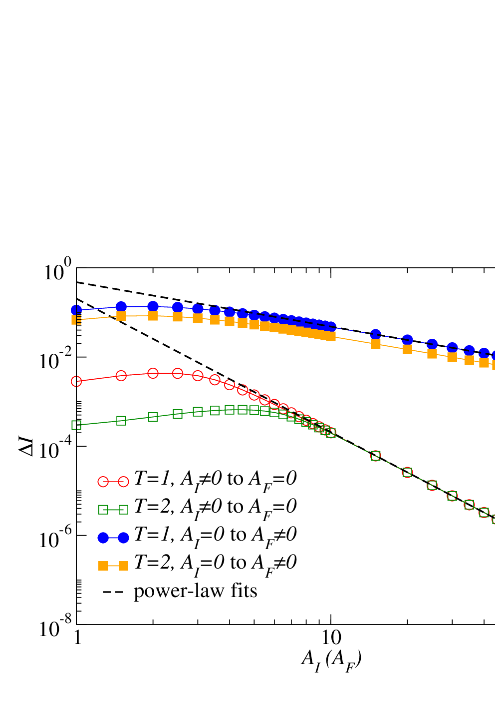
The dependence of on (), for a fixed system size and for two different temperatures, is depicted in Fig. 10. For both kinds of quenches, one can see that vanishes as a power law in the regime of large : for the quench from to , decreases as , while for the opposite quench it decreases as . One should note that, as expected from the discussion in Sec. IV, the behavior seen for is independent of and identical to that in the ground state. The exponents of the power laws are also independent of for both quenches and are found to be one-half those for vs .
as a function of is shown in Fig. 11, for three quenches and for three quenches . The behavior of is once again similar to that observed for vs in the same quenches; vanishes as a power law at very high temperatures. Power-law fits in the region yield for quenches and for quenches . Once again, the exponents are found to be one-half those for vs in Sec. IV.

The preceding analysis clearly shows that only when the difference between the conserved quantities in the initial state (in the GGE) and those in the thermal ensembles becomes negligible do the entropies and the ensembles themselves become equivalent. An understanding of this, as well as of the relation between the exponents of the power-law decays seen for and , can be gained if one realizes that the entropy in the GGE and the GE can be written in terms of the occupations of the single-particle eigenstates as
| (17) |
where for the GGE and for the GE. Once the occupations in both ensembles are very close to each other, they are also very close to 1/2 (see Fig. 8). One can write and (with ); it is then straightforward to show that
| (18) |
which provides an excellent description of the results for in Sec. IV and decays with a power-law exponent that is twice that for .
VI conclusions
In this paper, we have studied properties of 1D lattice hard-core bosons ( chain) after quenches that start from initial thermal states. In all cases considered, the quenches were generated by sudden changes in a superlattice potential (a local space-dependent magnetic field in the spin language). We have shown that, in these integrable systems after a quench starting from a finite-temperature state, the coarse-grained energy densities exhibit a Gaussian shape. However, the distributions of the weights are still qualitatively different between the quenched state and thermal states. This dissimilarity leads to an extensive difference among the entropies in the isolated system after the quench (the diagonal entropy), the GGE, and the thermal ensembles. On the other hand, as one (or both) of the two control parameters explored here (the initial temperature and the strength of the superlattice or ) are tuned to infinity, all ensembles become equivalent. The approach between the entropy of the GE and that of the GGE under such tuning was shown to be power law in the control parameter, independent of the quench protocol selected and of the values of the other parameters that were kept fixed. It is important to emphasize that, when all parameters in the quenches were kept fixed and finite and the system size was extrapolated to infinity, the differences between the GGE and the GE results were seen to saturate at a finite value, i.e., these two ensembles do not become equivalent.
We have also shown that such differences have their origin in the disagreement between the conserved quantities after the quench, which are determined by the initial state, and the distribution of conserved quantities in thermal ensembles. By tuning the control parameters mentioned above to infinity, we have seen that the distribution of the conserved quantities in the quenched state approaches that in thermal equilibrium, which explains why the generalized and thermal ensembles approach each other under those conditions. However, we should stress that, in our particular systems of interest and quench protocols followed, thermalization only occurs when the control parameters are tuned to lead to completely flat distributions of conserved quantities, which is what happens when the initial temperature is infinite or when .
Acknowledgements.
This work was supported by the U.S. Office of Naval Research. We thank Juan Carrasquilla for useful discussions.References
- [1] M. Greiner, O. Mandel, T. Hänsch, and I. Bloch, Nature 419, 51 (2002).
- [2] T. Kinoshita, T. Wenger, and D. Weiss, Nature 440, 900 (2006).
- [3] S. Hofferberth, I. Lesanovsky, B. Fischer, T. Schumm, and J. Schmiedmayer, Nature 449, 324 (2007).
- [4] S. Will, T. Best, U. Schneider, L. Hackermüller, D.-S. Lühmann, and I. Bloch, Nature 465, 197 (2010).
- [5] S. Trotzky, Y.-A. Chen, A. Flesch, I. P. McCulloch, U. Schollwöck, J. Eisert, and I. Bloch, Nature Phys. 8, 325 (2012).
- [6] M. Rigol, V. Dunjko, V. Yurovsky, and M. Olshanii, Phys. Rev. Lett. 98, 050405 (2007).
- [7] M. A. Cazalilla, Phys. Rev. Lett. 97, 156403 (2006).
- [8] M. Rigol, A. Muramatsu, and M. Olshanii, Phys. Rev. A 74, 053616 (2006).
- [9] P. Calabrese and J. Cardy, J. Stat. Mech. 2007, P06008 (2007).
- [10] M. Rigol, V. Dunjko, and M. Olshanii, Nature 452, 854 (2008).
- [11] M. Eckstein and M. Kollar, Phys. Rev. Lett. 100, 120404 (2008).
- [12] M. Kollar and M. Eckstein, Phys. Rev. A 78, 013626 (2008).
- [13] A. Iucci and M. A. Cazalilla, Phys. Rev. A 80, 063619 (2009).
- [14] D. Rossini, A. Silva, G. Mussardo, and G. E. Santoro, Phys. Rev. Lett. 102, 127204 (2009).
- [15] D. Rossini, S. Suzuki, G. Mussardo, G. E. Santoro, and A. Silva, Phys. Rev. B 82, 144302 (2010).
- [16] D. Fioretto and G. Mussardo, New J. Phys. 12, 055015 (2010).
- [17] A. Iucci and M. A. Cazalilla, New J. Phys. 12, 055019 (2010).
- [18] J. Mossel and J.-S. Caux, New J. Phys. 12, 055028 (2010).
- [19] A. C. Cassidy, C. W. Clark, and M. Rigol, Phys. Rev. Lett. 106, 140405 (2011).
- [20] P. Calabrese, F. H. L. Essler, and M. Fagotti, Phys. Rev. Lett. 106, 227203 (2011).
- [21] M. Rigol and M. Fitzpatrick, Phys. Rev. A 84, 033640 (2011).
- [22] M. A. Cazalilla, A. Iucci, and M.-C. Chung, Phys. Rev. E 85, 011133 (2012).
- [23] M. Kormos, A. Shashi, Y.-Z. Chou, and A. Imambekov, arXiv:1204.3889v1 (2012).
- [24] M. Cramer, C. M. Dawson, J. Eisert, and T. J. Osborne, Phys. Rev. Lett. 100, 030602 (2008).
- [25] T. Barthel and U. Schollwöck, Phys. Rev. Lett. 100, 100601 (2008).
- [26] E. T. Jaynes, Phys. Rev. 106, 620 (1957a).
- [27] E. T. Jaynes, Phys. Rev. 108, 171 (1957b).
- [28] J. M. Deutsch, Phys. Rev. A 43, 2046 (1991).
- [29] M. Srednicki, Phys. Rev. E 50, 888 (1994).
- [30] J. Berges, S. Borsányi, and C. Wetterich, Phys. Rev. Lett. 93, 142002 (2004).
- [31] M. Moeckel and S. Kehrein, Phys. Rev. Lett. 100, 175702 (2008).
- [32] M. Eckstein, M. Kollar, and P. Werner, Phys. Rev. Lett. 103, 056403 (2009).
- [33] M. Moeckel and S. Kehrein, Ann. Phys. 324, 2146 (2009).
- [34] M. Kollar, F. A. Wolf, and M. Eckstein, Phys. Rev. B 84, 054304 (2011).
- [35] M. Rigol and M. Srednicki, Phys. Rev. Lett. 108, 110601 (2012).
- [36] S. Deng, G. Ortiz, and L. Viola, Phys. Rev. B 83, 094304 (2011).
- [37] M.-C. Chung, A. Iucci, and M. A. Cazalilla, arXiv:1203.0121v1 (2012).
- [38] T. Holstein and H. Primakoff, Phys. Rev. 58, 1098 (1940).
- [39] P. Jordan and E. Wigner, Z. Phys. 47, 631 (1928).
- [40] M. Rigol and A. Muramatsu, Phys. Rev. A 70, 031603(R) (2004).
- [41] M. Rigol and A. Muramatsu, Phys. Rev. A 72, 013604 (2005a).
- [42] K. He and M. Rigol, Phys. Rev. A 83, 023611 (2011).
- [43] K. He, I. I. Satija, C. W. Clark, A. M. Rey, and M. Rigol, Phys. Rev. A 85, 013617 (2012).
- [44] M. Rigol, Phys. Rev. A 72, 063607 (2005).
- [45] M. Rigol and A. Muramatsu, Mod. Phys. Lett. 19, 861 (2005b).
- [46] A. Polkovnikov, Ann. Phys. 326, 486 (2011).
- [47] L. F. Santos, A. Polkovnikov, and M. Rigol, Phys. Rev. Lett. 107, 040601 (2011).