Hyperelastic cloaking theory: Transformation elasticity
with pre-stressed solids
Abstract
Transformation elasticity, by analogy with transformation acoustics and optics, converts material domains without altering wave properties, thereby enabling cloaking and related effects. By noting the similarity between transformation elasticity and the theory of incremental motion superimposed on finite pre-strain it is shown that the constitutive parameters of transformation elasticity correspond to the density and moduli of small-on-large theory. The formal equivalence indicates that transformation elasticity can be achieved by selecting a particular finite (hyperelastic) strain energy function, which for isotropic elasticity is semilinear strain energy. The associated elastic transformation is restricted by the requirement of statically equilibrated pre-stress. This constraint can be cast as constant, where is the deformation gradient, subject to symmetry constraints, and its consequences are explored both analytically and through numerical examples of cloaking of anti-plane and in-plane wave motion.
1 Introduction
The principle underlying cloaking of electromagnetic and acoustic waves is the transformation or change-of-variables method [1, 2] whereby the material properties of the cloak are defined by a spatial transformation. While the first applications were to electromagnetism, e.g. [3], it was quickly realized that the same mathematical methods work equally well in acoustics [4, 5, 6]. The fundamental identity underlying electromagnetic and acoustic transformation is the observation that the Laplacian in the original coordinates maps to a differential operator in the physical coordinates that involves a tensor which can be interpreted as the new, transformed, material properties [7]. The equivalence between the Laplacian in the original coordinates and the new operator involves an arbitrary divergence free tensor [8], implying for the acoustic case that the transformed material properties are not unique. For a given transformation function one can achieve acoustic cloaking by a variety of materials, ranging from fluids with anisotropic inertia, to quasi-solids with isotropic density but anisotropic stiffness [8, 9]. Non-uniqueness of the material properties does not apply in the electromagnetic case, where, for instance, the permittivity and permeability tensors must be proportionate for a transformation of the vacuum.
A crucial aspect of transformation optics and acoustics is that the mapped properties correspond to exotic material properties far removed from the realm of the original material. This aspect is accentuated in transformation elasticity. In the first study of transformation theory to elastodynamics, Milton et al. [10] concluded that the transformed materials are described by the Willis model. This constitutive theory for material response is dispersive, involving coupling between stress and velocity, in addition to anisotropic inertia [11, 12]. Brun et al. [13] considered the transformation of isotropic elasticity in cylindrical coordinates and found transformed material properties with isotropic inertia and elastic behavior of Cosserat type. The governing equations for Cosserat elastic materials [14] are the same as those of “normal” linear elasticity except that the elastic moduli do not satisfy the minor symmetry, i.e. (although they do satisfy the major symmetry ). This implies a non-symmetric stress, which depends not only on the strain (the symmetric part of the displacement gradient) but also on the local rotation .
A thorough analysis of transformation theory for elasticity [15] indicates that, as in acoustics, the range of mapped material properties is highly non-unique, thus explaining the divergence in the previously obtained results [10, 13]. The transformed elastodynamic constitutive parameters may be characterized through their dependence on (i) the transformation (mapping function) and (ii) on the relation between the displacement fields in the two descriptions, represented by matrices: , the deformation matrix, and , respectively. It was shown [15] that requiring stress to be symmetric implies and that the material must be of Willis form, as Milton et al. [10] found. Setting , on the other hand, results in Cosserat materials with non-symmetric stress but isotropic density, as found by Brun et al. [13] and by Vasquez et al. [16]. An alternative approach to transformation elasticity has been proposed that employs inextensible fibers embedded in an elastic material [17, 18]. This has the advantage that the effective material has isotropic density and retains both the minor and major symmetries of the stiffness tensor. Despite the non-unique nature of transformation elasticity the materials required are, in all cases, outside the usual realms of possibility.
In this paper we consider a class of materials displaying non-symmetric stress of the type necessary to achieve elastodynamic cloaking. Effective moduli with the major symmetry that do not display the minor symmetry are found in the theory of incremental motion superimposed on finite deformation [19]. We take advantage of the similarities between transformation elasticity and small-on-large motion in the presence of finite pre-strain. The starting point is the formal equivalence of the constitutive parameters of transformation elasticity with the density and moduli for incremental motion after finite prestress. This offers the possibility for achieving elasticity of the desired form by proper selection of the finite (hyperelastic) strain energy function. Such an approach has been shown to be successful in the context of antiplane (SH) wave motion. By using the neo-Hookean strain energy for incompressible solids and applying a radially symmetric cylindrical pres-strain, Parnell [20] and Parnell et al. [21] showed that the resulting small-on-large equations are identically those required for cloaking of the SH wave motion. Here we consider the more general elastic transformation problem, including but not limited to SH motion. We show that the form of the finite strain energy is restricted in form for isotropic elasticity. The equivalence between the transformation and the finite pre-strain also limits the type of transformation possible. This contrasts with the acoustic and electromagnetic problems for which the transformation is arbitrary. The elastic transformation is restricted in form because the pre-stress must be statically equilibrated, implying that the transformation must satisfy a partial differential equation. We show that this constraint can be cast as constant, (subject to symmetry constraints), and explore its consequences both analytically and numerically.
We begin in §2 with a review of transformation elasticity and of incremental motion superimposed on finite pre-strain, emphasizing equivalence of the theories. The form of the finite strain energy necessary to achieve transformation elasticity is deduced in §3 and in §4 the constraint on the deformation for isotropic elasticity is derived. §5 presents a detailed example of the type of radially symmetric finite pre-strain possible for isotropic elasticity. These analytical results are extended and illustrated in §6 through numerical examples of cloaking of anti-plane and in-plane wave motion. Conclusions are presented in §7.
2 Background equations
We first review the theory of transformation elasticity for linearly elastic solids, and then consider the separate theory for incremental deformation in finite elasticity.
2.1 Review of transformation elasticity
2.1.1 Transformation notation
A transformation from the virtual configuration, , to the present configuration (also known as the physical or current domain) is described by the mapping from to . Component subscripts in upper and lower case are used to distinguish between explicit dependence upon and , and the summation convention on repeated subscripts is assumed. The transformation or mapping is assumed to be one-to-one and invertible. Perfect cloaking requires that the transformation is one-to-many at a single point in . This can be avoided by considering near-cloaks, where, for instance, a small hole in is mapped to a larger hole in .
The transformation gradient is defined as with inverse , or in component form , . The Jacobian of the transformation is . The infinitesimal displacement and stress are assumed to satisfy the equations of linear elasticity in the virtual domain:
| (1) |
where is the (scalar) mass density and the elements of the elastic stiffness tensor satisfy the full symmetries , ; the first identity expresses the symmetry of the stress and the second is the consequence of an assumed strain energy density function.
Particle displacement in the transformed domain, , is assumed to be related to the displacement in the virtual domain by the non-singular matrix as
| (2) |
The choice of the transpose, in eq. (2), means that the “gauge” and the transformation gradient are similar objects, although at this stage they are unrelated. Neither or are second order tensors because of the fact that they each have one “leg” in both domains. Milton et al. [10] specify since this is the only choice that guarantees a symmetric stress (see §2.1.2). Identifying [10] and with and , respectively, and using would lead one to expect . However, the displacements are not associated with the coordinate transformation and and are independent quantities.
2.1.2 The transformed equations of elasticity
Under the transformation (or change of coordinates) the equilibrium and constitutive relations (1) transform to [15]
| (3) |
with parameters , and defined as follows in the Fourier time domain (dependence understood but omitted)
| (4) | ||||
where . The elastic moduli and the density satisfy the symmetries
| (5) |
although these are not the full symmetries for the Willis constitutive model (which requires the additional “minor” symmetry ). Equations (3)-(4) are the fundamental result of elastic transformation theory [15].
The absence of the minor symmetries under the interchange of and in and of (4) implies that the stress is generally asymmetric. Symmetric stress is guaranteed if , and occurs if the gauge matrix is of the form , for any scalar , which may be set to unity with no loss in generality. This recovers the results of Milton et al. [10] that the transformed material is of the Willis form. As noted in [10], it is the only choice for that yields symmetric stress.
The equations in the transformed domain, which is the physical realm, clearly display a great deal of non-uniqueness, corresponding to a vast realm of possible material properties. Our preference is for non-dispersive (i.e. independent of frequency) materials, in particular, those with the least “unusual” properties, so that they can conceivably be related to actual materials. In this regard, isotropic density is achieved by taking the constant matrix proportional to the identity, , with without loss of generality. In this case , , with non-dispersive density and elastic moduli given by
| (6) |
The equations of motion in the current domain are then
| (7) |
The effective moduli of (6) satisfy the major symmetry (5)1 but , indicating a non-symmetric stress. Departure from symmetric stress is possible in continuum theories such as Cosserat elasticity and micropolar theories of elasticity. Another context admitting non-symmetric stress is the theory of small-on-large motion, described next.
2.2 Small-on-large theory
The solid material is considered in two distinct states: first, the reference configuration of the solid under zero strain, , and secondly the current state of the material, which is again identified with . The hyperelastic theory of small motion superimposed upon large depends upon the initial finite, i.e. large, static pre-strain which maps to . The subsequent small motion is defined by the dynamic mapping . The following theory assumes and the associated strain are sufficiently small that tangent moduli can be employed to derive the linear equations of motion for the small-on-large motion [19].
Towards that end we introduce the deformation gradient of the pre-strain with inverse , and Jacobian . The polar decomposition is , where is proper orthogonal (, ) and the tensors , Sym+ are the positive definite solutions of , . The material is assumed to be hyperelastic, implying the existence of a strain energy function per unit volume from which the static Cauchy pre-stress is defined as
| (8) |
The assumed dependence of on the deformation , along with the freedom to change the current coordinate basis (which has nothing to do with transformation!) implies that must depend upon for any orthogonal , and taking implies the dependence . Assuming the density in the reference configuration is , the governing equations for subsequent small-on-large motion then follow from the well known theory [19] as
| (9) |
where
| (10) |
3 Potential strain energy functions
Our objective is to find possible hyperelastic solids, i.e. strain energy functions such that the equations for small-on-large motion are equivalent to those required after transformation of a material assumed to be homogeneous with properties .
The connection between the transformation and the small-on-large theories is made by first identifying the displacement fields as equivalent, , and then requiring that the equations of motion (7) and (9) are the same. The latter is satisfied if
| (11) |
for some positive constant . Hence,
| (12) |
The reference density can then be chosen so that , and eq. (12) then implies that the hyperelastic material is defined by
| (13) |
Equation (13)1 is automatically satisfied if the transformation and the finite deformation are related in the following manner:
| (14) |
for some non-singular . Equation (13)2 combined with the expression for in eq. (10) yields a second order differential equation for the strain energy function,
| (15) |
Recall that and are constant, but at this stage the remaining quantities in (15), i.e. and , are not so constrained. The density in the reference configuration could be inhomogeneous, . In that case (15) would not have a general solution for unless also depends upon in such a manner that the right hand side is independent of . This suggests that permitting to be inhomogeneous does not provide any simplification, and we therefore take the reference density to be constant, although not necessarily the same as . The quantity could, in principle, be a matrix function of , but this makes the integration of (15) difficult if not impossible. We therefore restrict attention to constant . Consideration of the important case of isotropic elasticity in §4 indicates that the degrees of freedom embodied in do not provide any significant additional properties, and therefore for the remainder of the paper we take , and set with no loss in generality. In this case the solution of (15) such that under zero deformation is
| (16) |
Equation (16) provides a formal solution for , one that is consistent with (15). However, the dependence of in (16) upon points to a fundamental difficulty, since the strain energy should be a function of . The two are not equal in general, unless
| (17) |
We henceforth assume (17) to be the case: that is, we restrict consideration to deformations that are everywhere rotation-free. Equation (16) then suggests the following possible form of the finite strain energy
| (18) |
Although this has realistic dependence on , it will not in general satisfy eq. (15), i.e. . We return to this crucial point for isotropic elasticity in §4.3 where we demonstrate that eq. (15) is satisfied by the isotropic form of (18) under additional conditions. Note that the strain measure , which is sometimes called the extension tensor, has as conjugate stress measure where is the second Piola-Kirchhoff tensor [22, §2.5].
We restrict attention henceforth to the case of hyperelastic materials that are isotropic in the undeformed state.
4 Isotropic elasticity
4.1 Semilinear strain energy function
The initial moduli are with original Lamé moduli , and Poisson’s ratio . We consider the isotropic version of the hyperelastic strain energy in (18),
| (19) |
with the latter expression in terms of two of the three invariants of : , where , , are the principal stretches of . Materials with strain energy (19) have been called semilinear [23] because of its relative simplicity and the linear form of the Piola-Kirchhoff stress , related to the Cauchy stress by ; thus . John [24] proposed the strain energy (19) based on the explicit form of its complementary energy density in terms of , a property also noted by others [25, 26]. The semilinear strain energy is a special case of the more general harmonic strain energy function [24]. Plane strain solutions for harmonic strain energy are reviewed in [27, §5.2]. Sensenig [28] examined the stability of circular tubes under internal pressure, while Jafari et al. [29] considered both internal and external pressure loading. The latter study has implications for the stability of the pre-strain developed here, see §5.2.3.
The pre-stress follows from (8) as
| (20) |
It is emphasized that we are restricting attention to deformations with , so that the Piola-Kirchhoff stress is also symmetric with . Applying the equilibrium equation for the finite deformation,
| (21) |
We seek solutions with symmetric deformation gradient, , and hence . Consequently eq. (21) is satisfied by finite deformations satisfying either of the equivalent conditions and . Thus:
| (22) |
Since the two partial differential equations in (22) are the same we need only seek solutions of one. Focusing on we conclude that the most general type of deformation is described by
| (23) |
The appearance of the positive constant of integration in (23)1 means that the sum of the principal stretches is fixed,
| (24) |
Further implications of the general solution (23) for a material that is isotropic in its undeformed state is explored in greater detail in the next section. For now we note that the pre-stress follows from (20) and (24) as
| (25) |
4.2 The limit of
It is of interest to consider the limit of the isotropic solution for . By assumption the prestress must remain finite. Consequently, using eq. (25), it becomes clear that in the limit as the constant of integration , i.e.
| (26) |
where the scalar defines the constraint reaction stress (the factor is included for later simplification). The latter arises from the limiting process of in eq. (25), and has also been shown to be the unique form of the reaction stress for the constraint [30]. Note that in writing in (26) we maintain a term proportional to in the second term rather than incorporating it with the constraint term. This form is consistent with the requirement that and hence in the undeformed state . The equilibrium equation for the pre-strain follows from eq. (26) as , and since (see eq. (22)) it follows that constant.
Several aspects of (26) are noteworthy. The limit of is usually associated with incompressibility, i.e. the constraint or equivalently , although the reason underlying this identification originates in linear elasticity and is therefore by no means required. Strictly speaking, the isochoric constraint conserves volume under the deformation. Here we find that implies the kinematic constraint on the deformation that . The latter is associated with the notion of incompressibility in linear elasticity in the form and in the present context can be viewed as a “semilinear” feature, in keeping with the descriptor [23] for the strain energy function (19). The kinematic condition, or equivalently
| (27) |
has been called the Bell constraint [30] by virtue of the fact that Bell [31, 32] showed it to be consistent with numerous sets of data for metals in finite strain. Solids satisfying this constraint have been called Bell materials [30]. In contrast to the constraint it can be shown that volume decreases for every deformation of a Bell material, and hence isochoric deformations are not possible [30].
Another feature of the limit is that the strain energy in (26) has the functional dependence . It is interesting to compare this with the strain energy for a neo-Hookean solid, , associated with incompressibility (i.e. ). Both strain energies reduce to the incompressible form for linear elasticity, and the factor appearing in but not in can be attributed to the different constraints in each case ( or ). Parnell [20] and Parnell et al. [21] considered neo-Hookean materials in the context of transformation elasticity for isochoric deformation. The present results indicates that the same form of the strain energy but with a different constraint yields a quite distinct class of volume decreasing deformations. This aspect will be examined further in the next section in terms of specific examples.
4.3 Consistency condition
It remains to show that the semilinear strain energy (19) satisfies
| (28) |
Since the moduli are isotropic, it it sufficient to show the equivalence in any orthogonal system of coordinates. We choose the principal coordinate system, in which the non-zero components of for isotropic elasticity satisfy [19, eqs. (3.31)-(3.34)]
| (29a) | ||||
| (29b) | ||||
| (29c) | ||||
| (29d) | ||||
where , , with no summation on repeated indices. Using and as defined in eqs. (19) and (24) gives
| (30) | ||||
These satisfy (29a), (29c) and (29d). The remaining conditions (29b) become
| (31) |
Equation (31) constitutes three conditions, which taken together imply the unique but trivial solution , , i.e. zero pre-strain. We avoid this by restricting attention to two dimensional dynamic solutions only, either in-plane (P/SV) or out-of-plane (SH) motion.
4.3.1 In-plane (P/SV) motion
The small-on-large displacements for in-plane motion are of the form , , . The condition (31) then only needs to be satisfied in the single instance , implying that the out-of-plane extension is related to the sum of the in-plane extensions by
| (32) |
Since is strictly positive, this places an upper limit on the sum of the in-plane extensions: .
4.3.2 Out-of-plane (SH) motion
The out-of-plane SH motion is of the form , . The requirement now is that and are both equal to in order to recover the out-of-plane equation of motion and associated tractions. Using (29b) and (29c)
| (33) | ||||
where is the constant from eq. (24). In this form it is clear that if then in-plane pre-stretches must be the same, , and therefore all the stretches are constant (since is a constant). This rules out the possibility of SH cloaking since we require that the in-plane pre-strain be inhomogeneous. However, if both and simultaneously hold, then for inhomogeneous and unequal in-plane stretches and . We are therefore led to the conclusion that SH cloaking requires a separate limit of the semilinear strain energy, one satisfying the Bell constraint (27) for which the strain energy and stress are given by (26). Note that we do not get the neo-Hookean strain energy in this limit.
5 Applications to isotropic elasticity
5.1 Radially symmetric cylindrical deformations
Consider deformations that are radially symmetric, , , in cylindrical coordinates and . The stretch in the -direction is assumed fixed, constant. The deformation gradient for is irrotational with
| (34) |
where , and . The condition (24) implies that the sum of the in-plane principal stretches is constant, say , and the constraint (32) relates this to of eq. (27),
| (35) |
Equation (23) for reduces to an ordinary differential equation for ,
| (36) |
with general solution
| (37) |
Note that the free parameter may be expressed in terms of either or , using eqs. (32) and (35). Using eqs. (25), (36) and (34) it follows that the principal stretches and stresses for the radially symmetric cylindrical configuration are
| (38) | |||||
Note that
| (39) |
5.2 Two types of cloaking
5.2.1 Conventional cloaking (CC)
The conventional concept of a cloaking material is that it occupies a finite region, in this case, the shell which maps to an equivalent shell in physical space with the same outer surface and an inner surface of radius larger than the original, i.e. , . Applying (37) with the two constraints and yields
| (40) |
which specifies the previously free parameter (also and ) as
| (41) |
The constraint therefore sets a lower limit in the permissible value of the outer radius as
| (42) |
The mapping (40) must also be one-to-one within the shell with . This means that there should be no zero of for . The convex nature of the solution (40) implies there is only one zero, say at . Since sgnsgn, it follows that must hold. Noting from (37) that , and using (40) to infer and , the condition becomes
| (43) |
The magnification factor , which measures the ratio of the radius of the mapped hole to the radius of the original one, is therefore bounded according to
| (44) |
In order to achieve a reasonable degree of cloaking one expects that the magnification factor is large, so that the mapped hole corresponds to an original hole of small radius and hence small scattering cross-section. The limitation expressed by (44) therefore places a severe restriction on the use of the hyperelastic material as a conventional cloak. Note that the upper limit on in (43) is not strictly achievable because implies and hence the principal stresses become infinite at .
The hyperelastic mapped solid has other aspects that further diminish its attractiveness as a conventional cloaking material. Specifically, a non-zero traction must be imposed on both the outer and inner boundaries to maintain the state of prestress. Noting that the radial stress is
| (45) |
with given in (40), yields
| (46) |
The necessity of the inner traction at is a reasonable condition, but the requirement for an equilibrating traction at is physically difficult. One way to avoid this is to let , considered below.
Examples of the radial deformation are given in Figure 1.

5.2.2 Hyperelastic cloaking (HC)
The hyperelastic material is now considered as infinite in extent. The cloaking effect is caused by allowing a radially symmetric hole in the unstressed configuration to be expanded under the action of an internal pressure to become a larger hole. We therefore require that the traction at infinity is zero, and that tends to unity, so that (39) applies. Then setting the mapped hole radius to implies the unique mapping
| (47) |
This deformation is simply the limiting case of (40) for . Note that the restriction (44) still applies to the magnification factor , in order to ensure for . The traction at the inner surface is a pressure which follows from (46) in the limit , , as
| (48) |
It is interesting to note that the internal pressure is independent of the Poisson’s ratio and it is therefore the same as found by [20] considering SH incremental motion.
5.2.3 Stability of the pre-strain
Jafari et al. [29] examined the stability of a finite thickness tube composed of material with harmonic strain energy, which includes semilinear strain energy as a special case. They showed that radially symmetric two dimensional finite deformations are stable under interior pressurization with zero exterior pressure. This implies that the finite pre-strain HC is stable. The stability of the CC deformation (40) does not appear to have been considered, and remains an open question. However, the stability of the HC, corresponding to , means there exists a minimum for which CC stability is ensured for all .
5.3 The limiting case when
In this limit the constraint (27) applies and the pre-stress for the radially symmetric deformation follows from (26) with constant “pressure” (see §4.2) as
| (49) |
where the value of the constant depends on the specified boundary conditions, and , , with given by eq. (37) for , For instance, in the case of hyperelastic cloaking as defined in §5.2.2 we find, noting the result (39), that , yielding the same interior pressure as eq. (48).

6 Numerical examples
We illustrate the above theory in the two dimensional setting where we consider wave scattering from a cylindrical cavity with and without a cloak where the cloak is a conventional cloak created via pre-stress. We shall show that partial cloaking is achieved, in the sense that scattering is significantly reduced by presence of a cloak. We are not able to achieve perfect cloaking since the cavity has to be of finite radius initially and furthermore, the hyperelastic theory above restricts the expansion to be at most twice the initial radius, i.e. . We consider two cases: horizontally polarized shear (SH) waves and coupled compressional/in-plane shear (P/SV) waves. We take which upon using (43) gives an initial inner to outer cloak radius ratio and .
For the SH and P/SV wave examples considered below, we use the description in Appendices A.1 and A.2 regarding scattering from a cylindrical cavity in an undeformed medium due to an incident field generated by a line source. In both cases considered, we assume that the line source is located at a distance from the centre of the cavity with , it is of unit amplitude and in the P/SV case it generates purely compressional waves.
6.1 SH wave propagation
In this case the shear wavenumber of the medium is defined by where is the density of the medium in the undeformed configuration. We use the solution in Appendix A.1 to solve the corresponding (conventional, pre-stress) cloak problem, the difference arising merely due to the modified argument due to the hyperelastic deformation (and invariance of equations). We shall always consider the case when , the outer cloak boundary. Thus in the solution can be written as (A.2), noting that the scattering coefficients are equivalent to scattering coefficients for a cavity of radius . Therein resides the reduction in scattering. In , the total field is given by but with an argument given by
| (50) |
i.e. that corresponding to the hyperelastic deformation described above (see eq. (37)).
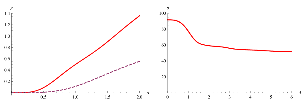
We take terms in the modal sum (A.2) for the wave field, sufficient for convergence of the solution. Figure 2 shows both the total (top) and scattered (bottom) fields corresponding to the following problems: scattering from a cavity of radius with in an undeformed medium (left) and scattering from a cavity with the presence of a hyperelastic cloak (right) with undeformed () and deformed () inner radii defined via where is defined above. The outer cloak boundary is defined by (right). This demonstrates significantly reduced scattering due to the presence of the hyperelastic cloak as compared with the non-cloaked case. Indeed we are able to quantify this by determining the reduction in scattering cross-section, defined in (A.3) for plane wave incidence. Without the cloak we have whereas with the cloak resulting in a reduction in scattering. Figure 3 shows the scattering cross-section (left) together with the percentage reduction in scattering (right).

6.2 P/SV wave propagation
In the P/SV case, in addition to the shear wavenumber we also introduce the compressional wavenumber via . We use the undeformed medium solution as derived in Appendix A.2 as a means of determining the solution for the cloak problem. This solution is employed in the exterior region together with the same solution but with modified argument (due to the hyperelastic deformation) in the cloak region. Thus in the solution can be written as (A.5) with scattering coefficients and given by (A.6a) and (A.6b) respectively, noting that they are equivalent to scattering coefficients for a cavity of radius and therefore a reduction in scattering is present. Note that here a different effect is introduced as compared with the SH case: shear waves are produced as a result of mode conversion on the boundary of the cavity. In , the total field is given by the sum of the scattered and incident fields but with the argument as given in (50) due to the hyperelastic deformation.
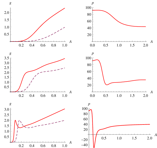
We take 30 terms in the modal sums (A.5), which is sufficient for convergence of the solution. Figure 4 shows the scattered fields corresponding to the P-wave (top) and S-wave (bottom) fields associated with and for the following problems: scattering from a cavity of radius with in an undeformed medium (left) and scattering from a cavity with the presence of a hyperelastic cloak (right) with undeformed () and deformed () inner radii defined via . The outer cloak boundary is defined by (right). Scattering is significantly reduced due to the presence of the hyperelastic cloak as compared with the non-cloaked case although it is relatively difficult to see this directly with the plots. As with the SH case, let us quantify this by determining the reduction in scattering cross-section, defined in (A.8) for plane wave incidence. Without the cloak whereas with the cloak resulting in a reduction in scattering. Figure 5 illustrates the scattering cross-section (left) together with the percentage reduction in scattering (right) compared for three different Poisson ratios: and . Note that for very low frequencies there is a huge reduction in scattering, close to . This tails off at higher frequencies but still remains at around reduction in scattering which is clearly significant. Reduction is larger for smaller Poisson ratios. We also note the rather interesting result that the peak in the cross-section actually induces an increase in scattering at some values of as compared with the case without the cloak although this is only for a narrow range of such values. This can be associated with the increasing disparity in the P and and SV wave numbers as tends to , noting that .
7 Conclusions
The close correspondence between transformation elasticity and small-on-large theory points to a method for realizing the former. Specifically, the semilinear strain energy function of eq. (19) yields the correct incremental moduli required for transformation of isotropic elasticity. The connection between the two theories is that the transformation equals the finite deformation. The fact that the pre-stress must be in a state of equilibrium places a constraint on the type of transformations allowed. Specifically, they are limited by the condition (24), or equivalently, constant, which yields stable radially symmetric pre-strain [29]. This implies that the actual size of a cylindrical target can be increased in area by a factor of 4, its radius by factor of two, without any change to the scattering cross-section. The restricted form of the transformation is not surprising considering the fact that the theory can simultaneously control more than one wave type, in contrast to acoustics.
In the two-dimensional problems for which results were provided, it was shown that the presence of a conventional cloak generated by the use of pre-stress leads to a significant reduction in the scattering cross-section from the cavity, as compared with scattering from a cavity without a cloak. This effect is particularly striking at low frequencies and for small Poisson ratios. We should note that in general one has to consider stability of nonlinear elastic solids in the large deformation regime. While we have not undertaken a full stability analysis, we have noted that the deformation for what we have termed hyperelastic cloaking (HC) is automatically stable (see §5.2.3). Extension of these results will be the subject of subsequent study. We also note that manufacturing nonlinear elastic solids with specific strain energy functions can be difficult to achieve in practice, although this is certainly no harder than generating complex metamaterials which appears to be the current alternative.
This work sheds some light on transformation methods in other wave problems. In acoustics and electromagnetism there is no constraint on the transformation; any one-to-one mapping is permitted. In principle, there is no constraint for transformation elasticity either, although the transformed materials are quite difficult if not impossible to obtain, especially since they are required to lose the minor symmetry in their corresponding elastic modulus tensor. The equivalence of transformation elasticity and small-on-large theory provides a unique and potentially realizable solution, although with a limited range of transformations allowed. It would be desirable to relax this constraint, which interestingly, does not appear for the related problem of SH wave motion in incompressible hyperelastic solids [20]. The limit of incompressibility offers a clue to a possible resolution for solids with Poisson’s ratio close to one-half, and will be the subject of a separate study.
Appendix
A Elastic wave scattering from cylindrical cavities
Brief summaries of the two wave scattering problems are given below. For further details see e.g. Eringen and Suhubi [33]. Scattering is considered from a cylindrical cavity of radius , located at the origin of a Cartesian coordinate system , related to a cylindrical polar coordinate system via . An incident wave is generated by a line source of amplitude (a force per unit length) located at the point . We take , subtended from the positive axis.
A.1 SH wave scattering
In this case the line source is polarized in the direction thus creating incident horizontally polarized shear (SH) waves which are then scattered from the cavity without mode conversion. The total wave field in this domain will therefore be where satisfies
| (A.1) |
with and . We seek in the form where is the incident field and with . We have defined , the Hankel function of the first kind, noting that and are Bessel functions of the first and second kind respectively, of order zero. Together with the time dependence in the problem, this ensures an outgoing field from the source. Graf’s addition theorem allows us to write this field relative to the coordinate system centred at the origin of the cavity [34] and we can use the form appropriate on in order to enforce the traction free boundary condition on , yielding the scattered field in the form
| (A.2) |
where and are respectively Hankel and Bessel functions of the first kind of order . We have also defined , , . If we take and , the incident wave of unit amplitude takes the (plane-wave) form where is the angle of incidence subtended from the negative axis. The scattered wave takes the form (A.2)1 with . The scattering cross-section of the cylindrical cavity for plane wave incidence is [35]
| (A.3) |
A.2 P/SV wave scattering
In this case the line source at with amplitude is a compressional source. Thus the incident field consists purely of in-plane compressional waves. Due to mode conversion, the scattered field consists of coupled in-plane compressional (P) and vertically polarized shear (SV) waves. The total wave field will therefore be and using the Helmholtz decomposition , we deduce that
| (A.4) |
where , and . Seek the wave field in the form where is the incident compressional wave with notation defined in Appendix A.1. We satisfy the traction free (, ) boundary condition on , by using Graf’s addition theorem, and the scattered field is
| (A.5) |
The scattering coefficients are
| (A.6a) | ||||
| (A.6b) | ||||
where
| (A.7) | ||||
If we take together with the incident wave of unit amplitude takes the (plane-wave) form where is defined above in Appendix A.1. The plane wave scattered fields take the form in (A.5) with where the latter are given defined in (A.6) under the replacement . The scattering cross-section of the cylindrical cavity for plane compressional wave incidence (subscript indicating this fact) is [35]
| (A.8) |
Acknowledgments
We would like to thank Ellis Dill for comments and suggestions. The work of ANN was supported by the Office of Naval Research and by the National Science Foundation.
References
- [1] A. Greenleaf, M. Lassas, and G. Uhlmann. On nonuniqueness for Calderon’s inverse problem. Math. Res. Lett., 10:685–693, 2003.
- [2] J. B. Pendry, D. Schurig, and D. R. Smith. Controlling electromagnetic fields. Science, 312(5781):1780–1782, 2006.
- [3] D. Schurig, J. J. Mock, B. J. Justice, S. A. Cummer, J. B. Pendry, A. F. Starr, and D. R. Smith. Metamaterial electromagnetic cloak at microwave frequencies. Science, 314(5801):977–980, 2006.
- [4] S. A. Cummer and D. Schurig. One path to acoustic cloaking. New J. Phys., 9(3):45+, 2007.
- [5] H. Chen and C. T. Chan. Acoustic cloaking in three dimensions using acoustic metamaterials. Appl. Phys. Lett., 91(18):183518+, 2007.
- [6] S. A. Cummer, B. I. Popa, D. Schurig, D. R. Smith, J. Pendry, M. Rahm, and A. Starr. Scattering theory derivation of a 3D acoustic cloaking shell. Phys. Rev. Lett., 100(2):024301+, 2008.
- [7] A. Greenleaf, Y. Kurylev, M. Lassas, and G. Uhlmann. Full-wave invisibility of active devices at all frequencies. Comm. Math. Phys., 275(3):749–789, 2007.
- [8] A. N. Norris. Acoustic cloaking theory. Proc. R. Soc. A, 464:2411–2434, 2008.
- [9] A. N. Norris. Acoustic metafluids. J. Acoust. Soc. Am., 125(2):839–849, 2009.
- [10] G. W. Milton, M. Briane, and J. R. Willis. On cloaking for elasticity and physical equations with a transformation invariant form. New J. Phys., 8:248–267, 2006.
- [11] J. R. Willis. Dynamics of composites, volume 495 of Continuum Micromechanics: CISM Lecture Notes, chapter 1, pages 265–290. Springer, Wien/New York, 1997.
- [12] G. W. Milton and J. R. Willis. On modifications of Newton’s second law and linear continuum elastodynamics. Proc. R. Soc. A, 463(2079):855–880, 2007.
- [13] M. Brun, S. Guenneau, and A. B. Movchan. Achieving control of in-plane elastic waves. Appl. Phys. Lett., 94:061903, 2009.
- [14] E. Cosserat and F. Cosserat. Théorie des Corps Déformables. Librairie Scientifique A. Hermann et fils, Paris. ISBN 978-1429704847, reprinted by Cornell University Library, 1909.
- [15] A. N. Norris and A. L. Shuvalov. Elastic cloaking theory. Wave Motion, 49:525–538, 2011.
- [16] F. G. Vasquez, G. W. Milton, D. Onofrei, and P. Seppecher. Transformation elastodynamics and active exterior acoustic cloaking. In S. Guenneau and R. Craster, editors, Acoustic Metamaterials: Negative Refraction, Imaging, Lensing and Cloaking, pages 1–1. Canopus Academic Publishing and Springer SBM, 2012.
- [17] P. Olsson and D. J. N. Wall. Partial elastodynamic cloaking by means of fiber-reinforced composites. Inverse Problems, 27(4):045010+, 2011.
- [18] P. Olsson. Non-uniqueness of time-domain reflection from 3D planar elastic layers. Wave Motion, 48:539–549, 2011.
- [19] R. W. Ogden. Incremental statics and dynamics of pre-stressed elastic materials. In M. Destrade and G. Saccomandi, editors, Waves in Nonlinear Pre-Stressed Materials: CISM International Centre for Mechanical Sciences, volume 495, chapter 1, pages 1–26. Springer, 2007.
- [20] W. J. Parnell. Nonlinear pre-stress for cloaking from antiplane elastic waves. Proc. R. Soc. A, 468:563–580, 2012.
- [21] W. J. Parnell, A. N. Norris, and T. Shearer. Employing pre-stress to generate finite cloaks for antiplane elastic waves. Appl. Phys. Lett., In press, 2012.
- [22] E. H. Dill. Continuum Mechanics: Elasticity, Plasticity, Viscoelasticity. CRC Press, 2007.
- [23] AI Lur’e. Theory of elasticity for a semilinear material. Prikl. Mat. Mekh (J. Appl. Math. Mech.), 32:1053–1069 (1068–1085), 1968.
- [24] F. John. Plane strain problems for a perfectly elastic material of harmonic type. Comm. Pure Appl. Math., 13(2):239–296, 1960.
- [25] L. M. Zubov. The stationary principle of complementary work in non-linear theory of elasticity. Prikl. Mat. Mekh (J. Appl. Math. Mech.), 34:241–245 (228–232), 1970.
- [26] I. Raasch. A variational principle for non-linear elastodynamics and its application to the hybrid stress model. Int. J. Nonlinear Mech., 10(5):215–222, 1975.
- [27] R. W. Ogden. Non-Linear Elastic Deformations. Dover Publications, 1997.
- [28] C. B. Sensenig. Instability of thick elastic solids. Comm. Pure Appl. math., 17(4):451–491, 1964.
- [29] A. H. Jafari, R. Abeyaratne, and C. O. Horgan. The finite deformation of a pressurized circular tube for a class of compressible materials. Z. Angew. Math. Phys., 35(2):227–246, March 1984.
- [30] M. F. Beatty and M. A. Hayes. Deformations of an elastic, internally constrained material. Part 1: Homogeneous deformations. J. Elasticity, 29(1):1–84, 1992.
- [31] J. F. Bell. Contemporary perspectives in finite strain plasticity. Int. J. Plasticity, 1:3–27, 1985.
- [32] J. F. Bell. Experiments on the kinematics of large plastic strain in ordered solids. Int. J. Solids Struct., 25:267–277, 1989.
- [33] A.C. Eringen and E.S. Suhubi. Elastodynamics, Vol. II. Academic Press, New York, 1975.
- [34] P. A. Martin. Multiple Scattering: Interaction of Time-harmonic Waves with N Obstacles. Cambridge University Press, New York, 2006.
- [35] T.S. Lewis, D.W. Kraft, and N. Hom. Scattering of elastic waves by a cylindrical cavity in a solid. J. Appl. Phys., 47(5):1795–1798, 1976.