Providing End-to-End Delay Guarantees for Multi-hop Wireless Sensor Networks over Unreliable Channels
Abstract
Wireless sensor networks have been increasingly used for real-time surveillance over large areas. In such applications, it is important to support end-to-end delay constraints for packet deliveries even when the corresponding flows require multi-hop transmissions. In addition to delay constraints, each flow of real-time surveillance may require some guarantees on throughput of packets that meet the delay constraints. Further, as wireless sensor networks are usually deployed in challenging environments, it is important to specifically consider the effects of unreliable wireless transmissions.
In this paper, we study the problem of providing end-to-end delay guarantees for multi-hop wireless networks. We propose a model that jointly considers the end-to-end delay constraints and throughput requirements of flows, the need for multi-hop transmissions, and the unreliable nature of wireless transmissions. We develop a framework for designing feasibility-optimal policies. We then demonstrate the utility of this framework by considering two types of systems: one where sensors are equipped with full-duplex radios, and the other where sensors are equipped with half-duplex radios. When sensors are equipped with full-duplex radios, we propose an online distributed scheduling policy and proves the policy is feasibility-optimal. We also provide a heuristic for systems where sensors are equipped with half-duplex radios. We show that this heuristic is still feasibility-optimal for some topologies.
Index Terms:
Wireless sensor networks; end-to-end deadline; real-time communicationsI Introduction
The advance of wireless sensor networks provides an appealing solution for real-time surveillance. In real-time surveillance, wireless sensors generate flows of surveillance data and deliver them to a sink, which makes control decisions based on the data. Examples of such applications have been demonstrated in many previous work, such as [1, 2, 3].
A major challenge for real-time surveillance is to provide end-to-end delay guarantees for packet deliveries. Designing scheduling policies that provide end-to-end delay guarantees is difficult due to two reasons. As wireless sensor networks may be deployed over a large area, some flows may require multi-hop transmissions to reach the sink. Further, wireless sensor networks are usually deployed in challenging environments, such as battlefields, forests, or underwater. Within these environment, it may be impossible to ensure that all wireless transmissions can be successfully received. Thus, a desirable policy needs to explicitly address the unreliable nature of wireless transmissions.
In this paper, we aim to address the above difficulties. We measure the performance of each surveillance flow by its timely-throughput, defined as the throughput of packets that are delivered to the sink on time. We then propose a model that characterizes the hard per-packet end-to-end delay constraints and timely-throughput requirements of flows, the routing protocol for multi-hop transmissions, and the unreliable wireless channels. This model also considers both scenarios where sensors are equipped with full-duplex radios and half-duplex ones.
Based on the model, we establish a general framework for designing scheduling policies. We prove a sufficient condition for a scheduling policy to be feasibility-optimal, that is, to be able to fulfill all timely-throughput requirements as long as they are feasible. We show that, based on this condition, there is a dynamic programming approach for designing policies for various types of systems.
We then consider designing online, tractable, and distributed scheduling policies. We propose a policy for systems where sensors are equipped with full-duplex radios. We prove that the proposed policy is feasibility-optimal. We also propose a simple heuristic for systems where sensors are equipped with half-duplex radios, and show that it is feasibility-optimal among certain topologies.
In addition to theoretical studies, we also provide simulation results. We compare our proposed policies against other policies. Simulation results show that our proposed policies achieve significantly better performance than others.
The rest of the paper is organized as follows. Section II summarizes existing work on providing end-to-end delay guarantees. Section III formally introduces our analytical model. Section IV establishes a framework for designing feasibility-optimal policies. Based on the framework, Section V proposes a feasibility-optimal policy for systems where sensors are equipped with full-duplex radios. Section VI proposes a heuristic for systems where sensors are equipped with half-duplex radios, and proves that the heuristic is feasibility-optimal for some topologies. Section VII demonstrates our simulation results. Finally, Section VIII concludes this paper.
II Related Work
Providing end-to-end delay guarantees have been an important research topic for various systems. Jayachandran and Abdelzaher [4] have studied this problem for distributed real-time systems where a job needs to traverse a number of processors before it is completed, and have provided a worst-case analysis for end-to-end delays. Hong, Chantem, and Hu [5] have considered a similar problem and approached it by assigning local deadlines for each processor. Li and Eryilmaz [6] have proposed a scheduling policy that aims to meet per-packet delay bounds and timely-throughput requirements of flows in wireline networks. However, no performance guarantees were provided for their scheduling policy. Rodoplu et al [7] have studied the problem of estimating end-to-end delay over multi-hop wireless networks. Li et al [8] have proposed using expected end-to-end delay for selecting path in wireless mesh networks. The expected end-to-end delay takes both queuing delay and delay caused by unsuccessful wireless transmissions. However, their work only aims at minimizing the average end-to-end delays, and cannot provide guarantees on per-packet delays. Jayachandran and Andrews [9] have applied a coordinated EDF scheduler for wireless networks and obtained asymptotic bounds on end-to-end delays. Li et al [10] have used network calculus to analyze and derive upper-bound for end-to-end delays. Li, Li, and Mohapatra [11] have proposed a distributed policy for scheduling packets with end-to-end delay guarantees. However, their work lacks theoretical guarantees on performance.
There has also been a lot of work that considers end-to-end delay guarantees for wireless sensor networks. Jiang, Ravindran, and Cho [12] have studied the real-time capacity of wireless sensor networks. They approach this problem by decomposing end-to-end delays into per-hop delays, and then study the probability for meeting each per-hop delay independently. Wang et al [13] have used a similar decomposition approach and studied the problem of energy saving while providing end-to-end delay guarantees. Such decomposition approach inevitably leads to suboptimal solutions. Chipara et al [14] have proposed a protocol for scheduling real-time flows by taking interference among sensors into account. Wang et al [15] have investigated the distribution of end-to-end delay in wireless sensor networks. Wang et al [16] have formulated the problem of providing end-to-end delay guarantees as an optimization problem, and have proposed a heuristic for obtaining sub-optimal solutions. Li, Shenoy, and Ramamritham [17] have aimed at providing end-to-end delay guarantees by exploiting spatial reuse.
III System Model
In this section, we present our model for multi-hop wireless sensor networks with end-to-end delay constraints. Our model extends a model proposed in [18], which only considers the delay constraints of packets and unreliability of wireless transmissions in a one-hop scenario.
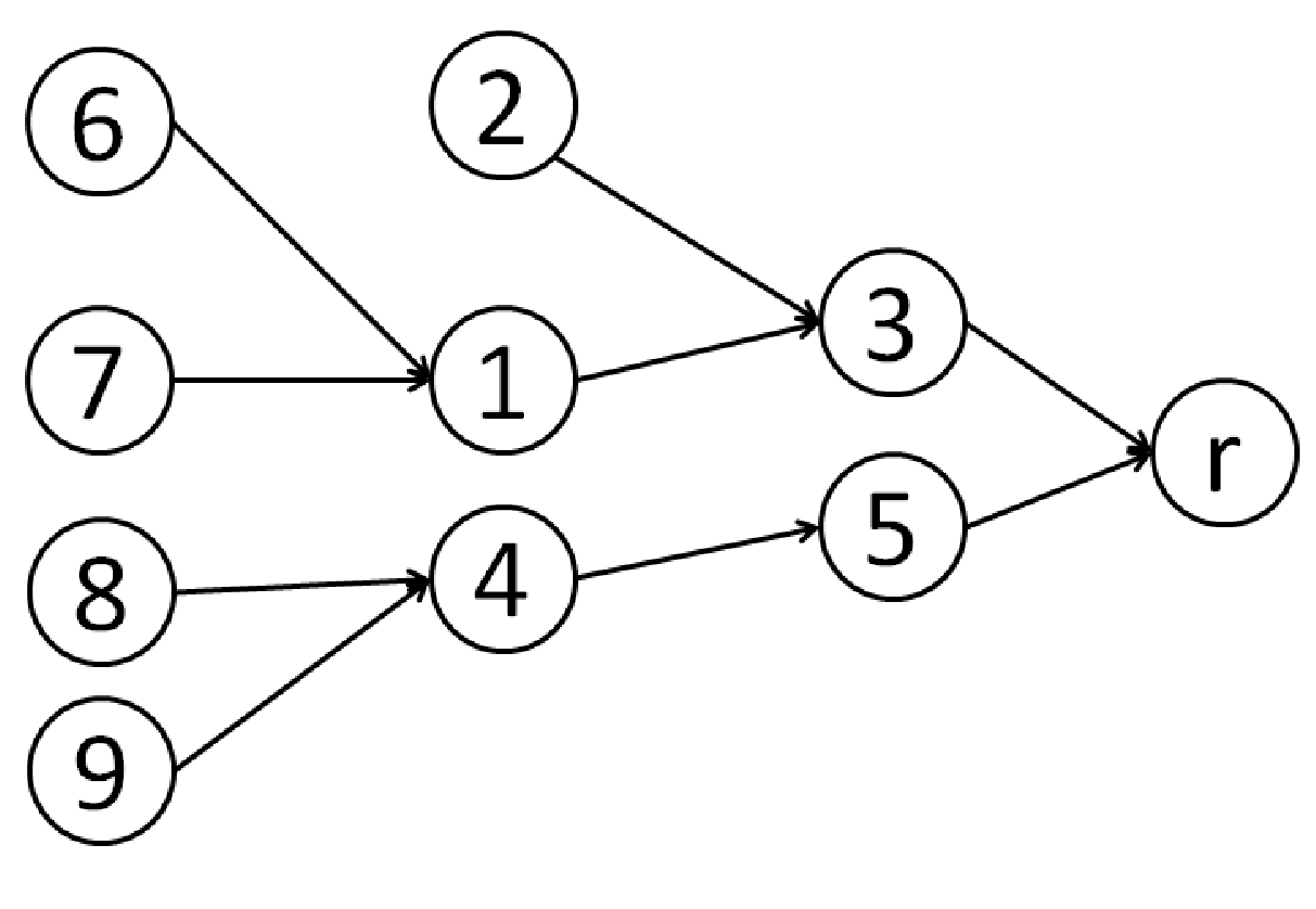
Consider a sensor network with a set of wireless sensors. One of the sensors play the role of the sink. Sensors may generate surveillance data that need to be delivered to the sink in a timely manner, and they may relay data that are generated by other sensors. We assume that a routing tree has been constructed by some routing protocol for the sensor network. There has been a lot of work on constructing routing trees for wireless sensor networks, and [19] provides a survey of these routing protocols. In the routing tree, the sink is the root, and hence we use to represent the sink. When a sensor has a data packet, either one generated by itself or one that is forwarded to it from other sensors, it may forward the data to its parent, denoted by , in the routing tree. Figure 1 shows an example of such a sensor network. A data packet is said to be delivered if it reaches the sink. A sensor may generate multiple flows of data. For example, one sensor may generate data on both temperature and humidity. We denote the set of flows in the wireless sensor network by , and as the sensor that generates data of flow .

We assume that time is slotted and numbered by . The length of a time slot is set to be the time needed for a sensor to transmit one data packet. Time slots are further grouped into intervals, where each interval consists of consecutive time slots in , for some . At the beginning of each interval, each flow in obtains some surveillance data and generates a data packet. We say that a the data packet of flow is generated at the time slot in each interval, so as to account for the latency caused by sensing and data processing. We assume that all data packets are delay-constrained, and data packets generated in one interval need to be delivered to the sink before the end of the interval. If a data packet is not delivered before the end of the interval, the packet is no longer useful for the sink. In this case, we say that the packet expires, and drop the packet from the system. Thus, we can guarantee that all data received by the sink have delays no larger than time slots.
We consider both cases when sensors are equipped with full-duplex radios and when they are equipped with half-duplex radios. When sensors are equipped with full-duplex radios, they can transmit and receive data packets simultaneously. We also assume that the transmissions of different sensors do not interfere with each other by, for example, allocating different sensors on different subcarriers in an orthogonal frequency-division multiple access (OFDMA) system. A system where sensors are equipped with full-duplex radios is called a full-duplex system.
The assumptions made for full-duplex systems may exceed current hardware limitations of wireless sensor network. Thus, we also consider systems where sensors are equipped with half-duplex radios. In such systems, sensors cannot transmit and receive data packets simultaneously. That is, when a sensor transmits, its parent cannot transmit, or the transmission by encounters a collision and the transmission fails. Moreover, we assume that a sensor can receive at most one transmission in a time slot. That is, if we have sensors and with , then at most one of them can transmit in a time slot. Finally, we assume that different transmissions do not interfere with each other except the two cases discussed above. This can be done by, for example, scheduling transmissions that may interfere with each other in different channels. A system where radios are equipped with half-duplex radios is called a half-duplex system.
We consider the unreliable nature of wireless transmissions. To be more specific, we say that when a sensor transmits a data packet to its parent, , correctly receives the packet with probability . We also assume that, by implementing ACKs, the sensor has feedback information on whether its transmission is correctly received by , and it can retransmit the same packet in the case that a previous transmission fails.
As wireless transmissions are unreliable, it may be impossible to deliver all data packets to the sink on time. Instead, each flow requires a portion of packets to be delivered on time. That is, let be the indicator function that the data packet of flow in the interval is delivered to the sink on time. Each flow then requires that, with probability one,
We call as the timely-throughput of flow up to interval , and as the timely-throughput requirement on flow .
In this paper, we aim to design scheduling policies that fulfills timely-throughput requirements of all flows as long as they are strictly feasible. These terms are formally defined as follows:
Definition 1
A system is said to be fulfilled by some scheduling policy if, under this policy, with probability one, for all flow .
Definition 2
A system, either a full-duplex system or a half-duplex one, is feasible if there exists some scheduling policy that fulfills it.
Definition 3
A system, either a full-duplex system or a half-duplex one, is strictly feasible if for all flows , and there exists some such that the system is still feasible when each flow requires a timely-throughput of .
Definition 4
A scheduling policy is feasibility-optimal for full-duplex system, or half-duplex system, if it fulfills all strictly feasible full-duplex systems, or all strictly feasible half-duplex systems, respectively.
We limit our discussions on strictly feasible systems only to simplify the proof of Theorem 1 in the following section. As can be arbitrarily small, this limitation is not restrictive.
IV A Framework for Scheduling Policies
In this section, we describe a sufficient condition for a policy to be feasibility-optimal. We then show a dynamic program approach that derives feasibility-optimal policies by employing this sufficient condition. This condition is based on the concept of debt:
Definition 5
The debt of in the interval is defined as , where is the indicator function that the packet for in interval is delivered on time.
It is easy to show that a system is fulfilled under some scheduling policy if and only if . Based on the concept of debt, we establish a sufficient condition for a policy to be feasibility-optimal for full-duplex systems or half-duplex systems. The condition is similar to the one introduced in [20], which only considers one-hop transmissions, and is based on the following theorem:
Lemma 1 (Telescoping Lemma)
Let be a non-negative Lyapunov function depending only on , which denotes the set of all events in the system in the first intervals, i.e., is adapted to . Suppose there exist positive constants , , and a stochastic process also adapted to , such that:
| (1) |
then , where is the expected value of .
Theorem 1
A scheduling policy is feasibility-optimal for full-duplex system, or half-duplex system, if, given , it maximizes
in the interval, for all , where , for all full-duplex systems, or half-duplex systems, respectively.
Proof:
Consider a strictly feasible system where flow requires a timely-throughput of . There exists some such that this system is fulfilled by some stationary randomized scheduling policy, , when each flow requires a timely-throughput of . Thus, under , we have .
Define a Lyapunov function . Since , we have
| (2) |
for some constant , as and are both bounded by 1, for all .
As under , for all , we have, under ,
| (3) |
IV-A A Dynamic Programming Approach for Scheduling Policies
We now introduce a dynamic programming approach for designing scheduling policies that aims at maximizing in the interval by making scheduling decisions for each time slot within the interval. We first describe the system evolution within an interval by a Markov decision process. In the time slot within the interval, we represent the state of the system by and the position of the packet of each flow. We denote the position of the packet of flow by , where if has the packet and can transmit it in the time slot, and if the packet of is yet to be generated, as the packet of flow will not be generated until the time slot in the interval. The evolution of can then be described as follows: when , where is the sensor that generates the packet of ; with probability if transmits the packet of in the time slot, where is the parent of in the routing tree and is the channel reliability between and ; and , otherwise.
We say that the interval ends when . Thus, the packet of is delivered, and , if . Let be the value of when the state of the system is represented by at the time slot under some policy. By Theorem 1, a policy is feasibility-optimal if it maximizes , where is the state of the system at the beginning of the interval. Let be the maximum value of . We then have the recursive relation: , where is the set of possible schedule decisions under the current state. Hence can be obtained by dynamic programming. Moreover, a policy that makes its schedule decisions by choosing for all states is feasibility-optimal.
While we can derive feasibility-optimal policies from the above approach, this approach may require high computation overhead, as the number of states for the system is as large as . In the following sections, we demonstrate that there is a simple online policy for full-duplex systems. We also introduce a heuristic for half-duplex system and show that the heuristic is feasibility-optimal under some restrictions.
V An Online Scheduling Policy for Full-Duplex Systems
We now introduce an online scheduling policy for full-duplex systems. The policy is very simple: in each time slot, a sensor picks the flow that has the largest debt among those that it currently holds their packets, and transmits its packet. In other words, in each time slot of the interval, schedules the packet from . We call this policy the Greedy Forwarder. In addition to low complexity, this policy is also distributed and does not require a centralized scheduler. Moreover, as we establish below, this simple policy is indeed feasibility-optimal.
Theorem 2
The Greedy Forwarder is feasibility-optimal.
Proof:
By Theorem 1, we can show that the Greedy Forwarder is feasibility-optimal by showing that it maximizes . To show this, we prove the following two claims by induction on the size of the network,:
- 1.
The Greedy Forwarder maximizes .
- 2.
Suppose a sensor generates packets from flow , where . Also assume that this sensor generates packets at time , and the sensor has control over which flow among is to generate packets at time , respectively. Then, with all other conditions fixed, by selecting to generate its packet at times , to generate its packet at time , etc, for the whole system is maximized.
We first discuss the case when , in which the sink is the only sensor in the system. As there is only one sensor in the system, there are no scheduling decisions to be made, and hence Claim (1) holds. Moreover, a packet of flow is delivered, and hence , if it is generated before the time slot. Thus, Claim (2) holds as is maximized by generating packets in decrement order of their debts.
Assume that both Claim (1) and Claim (2) hold for all networks with size . We now show that these two claims also hold for all networks with . We pick a leaf node, denoted by , in the routing tree. We assume that generates packets for flows , with , at times , and has control over which flows among is to generate packets at times , respectively. We also assume that uses a work-conserving policy, i.e., it always schedules a transmission as long as it holds a packet11 1 Obviously, a policy cannot lose its optimality by making more transmissions. Thus, this assumption is not restrictive.. Under this policy, successfully transmits packets at times . We note that are random variables whose distributions are determined by the channel reliability between and . Moreover, we have , for all , as it is impossible to successfully transmit packets before at least the same amount of packets are generated. Note that are not influenced by the order of packet generations and scheduling decisions, as each transmission made by is successful with probability , regardless which packet is being transmitted.
Given , can effectively determine which packets are to be successfully transmitted at times , by choosing the order of packet generations and scheduling decisions. The only restriction for is that the packet from a flow cannot be transmitted before it is generated. If the packet from a flow is successfully transmitted by at time , receives the packet at time and can transmit the packet starting at time . Thus, this system is equivalent to one with removed, making the size of the network to be , and packets from flows are generated at sensor at times . By the induction hypothesis on this system with sensors, is maximized if the packet from flow is generated at time , for all . As can make this happen by choosing flow to generate a packet at time and follow the Greedy Forwarder, both Claim (1) and Claim (2) hold when is included in the system with size .
By induction on , we have that both claims hold for all systems, and hence the Greedy Forwarder is feasibility-optimal. ∎
We close this section by discussing some implementation issues of the Greedy Forwarder. As noted above, under the Greedy Forwarder, every sensor makes scheduling decisions solely based on the packets it holds. Still, the Greedy Forwarder requires each sensor to have the knowledge of debts for all flows in the current interval. In practice, this may be impractical. In particular, for a large network, sensors that are far away from the sink can only obtain delayed information on debts of flows. However, as we will show in Section VII, when sensors apply the Greedy Forwarder with delayed information on debts, the resulting performance can still be optimal. This is because, as the net change of debt, , is bounded, the difference between the delayed information on debt and the actual current debt is also bounded for all flows. Therefore, a sensor that only has delayed information on debts will make similar scheduling decisions as one that has information on the current values of debts.
VI A Heuristic for Half-Duplex Systems
In this section, we propose a policy for half-duplex systems and show that this policy is feasibility-optimal for some particular scenarios.
Recall that there are two important limitations for half-duplex systems. First, as a sensor cannot transmit and receive simultaneously, a sensor cannot transmit when its parent, , is also transmitting. Second, a sensor can only receive one packet at a time, and hence two sensors and with cannot transmit simultaneously. To address theses challenges, we propose a policy, namely, the Closest Sensor First Policy. We first define . In other words, is the largest debt of flows that holds at the time slot. If the sensor does not hold any packets, is defined to be . The Closest Sensor First Policy can be described iteratively as follows: First, we examine all sensors that are one-hop away from the root , that is, we examine all sensors such that . We then schedule the sensor with the largest to transmit, and the sensor transmits the packet from the flow with the largest debt. Next, we examine sensors that are two-hop away from the root, that is, sensors with . If is scheduled to transmit in the first step, then cannot transmit. Otherwise, a sensor is scheduled to transmit the packet from the flow with the largest debt if is the largest among all sensors with . In the above procedure, ties are broken arbitrarily, and we carry the procedure iteratively.
In summary, a sensor who is -hop away from the root is scheduled in the iteration if: (i) is not scheduled in the previous iteration, and (ii) is the largest among all with . Fig. 2 shows an example that illustrates the Closest Sensor First Policy. In the example, we number sensors by their respective . Thus, we have . In the first iteration, sensor 5 is scheduled as . In the second iteration, sensor 2 is scheduled as . Note that sensor 4 cannot be scheduled as its parent, sensor 5, has already been scheduled. Finally, in the third iteration, sensor 7 and sensor 9 are scheduled.
Next, we show that the Closest Sensor First Policy is feasibility-optimal if all flows are generated by the same sensor , i.e., , for all , and each flow generates a packet at the beginning of the interval, i.e., , for all . In such a system, only sensors on the path between and are involved in forwarding messages. Thus, we call such a system as a path-topology system.
Theorem 3
The Closest Sensor First Policy is feasibility-optimal for path-topology systems.
Proof:
By Theorem 1, we can show that the Closest Sensor First Policy is feasibility-optimal for path-topology systems by establishing that this policy maximizes in the interval.
Let be the number of transmissions that sensor needs to make to successfully transmit packets to its parent. Note that this does not imply that sensor successfully transmits packets at the time slot in the interval, as there are time slots that sensor is not scheduled due to the constraints of half-duplex systems. We also note that is a geometric random variable with mean , as the channel reliability between and is . In practice, the values of cannot be obtained at the beginning of the interval. We will show that, even when the values of are given for all and , there is no policy that can achieve larger than the Closest Sensor First Policy, and hence than the Closest Sensor First Policy maximizes .
We order flows so that . Let and be the Closest Sensor First Policy and another policy that maximizes , respectively. Further, let and be the times that the packet from flow is delivered under and , respectively. If the packet from flow is not delivered on time under , or , we set , or , to be . Thus, under , or , we have , or , respectively.
By the design of the Closest Sensor First Policy, we have . Suppose there exists some so that under . We can modify so that whenever it schedules the packet from flow , it schedules the packet from flow instead, and vice versa. Under this modification, the packet of is delivered on the time slot, and the packet of is delivered on the time slot. If both and are smaller than , both packets are still delivered on time after this modification, and hence the value of is not influenced. If both and are larger than , neither packets are delivered on time after this modification, and the value of is not influenced. However, if , the packet of is delivered on time and the packet of is not after the modification, and the value of will not decrease, as , with the modification. In sum, the value of will not decrease with the modification. Thus, we can repeat this procedure until without decreasing the value of .
From now on, we assume that under . We claim that, under this assumption, for all . We prove this claim by induction on the number of flows. When there is only one flow in the system, the Closest Sensor First Policy schedules a transmission for flow 1 in every time slot, and hence .
Assume that for all when the system has flows. We now consider the case when the system has flows. Under the Closest Sensor First Policy, whether the packet of a flow with is scheduled is not influenced by whether the flow is present in the system. Thus, the value of is the same as in the case when the system only has flows, for all . We then have for all by the induction hypothesis. Therefore, we only need to prove that . If , i.e., the packet of flow is not delivered on time under , then holds.
Consider the case . Suppose that, under , there is some time during the interval when the packet from flow is closer to the root than the packet from flow , for some . Pick to be the smallest number so that the packet from flow is closer to the root than the packet from flow at some time during the interval. Now we can pick to be the largest time before such that the packet from flow and that from flow are held by the same sensor. Such exists as both packets are held by the sensor that generates all packets at the beginning of the interval. We then pick to be the smallest time after such that both packets are held by the same sensor. Such exists as we assume that the packet from flow is delivered earlier than the packet from flow . Thus, in any time slot in , the packet from flow is always closer to the root than that from flow . Now, we can modify for time slots in so that when it schedules , it schedules instead, and vice versa. After this modification, the packet from flow is always closer to the root than that from flow during . Further, this modification does not influence for any flow . We repeat this modification until such does not exist. From now on, we can assume that, at any point of time, the packet from flow is not closer to the root than the packet from flow if .
We prove that by contradiction. Note that after the packet of flow is delivered, , or , needs to schedule the packet of flow an addition number of , or , times before it is delivered, respectively. By the induction hypothesis, . Therefore, if , we have , and, under , there are times that the packet from flow is scheduled while it would not be schedule under . We call these times the inversion times and denote them by . We assume that, among all policies that deliver packets at times , is one that has the smallest number of inversion times. Moreover, among those policies that have the smallest number of inversion times, is one that maximizes .
At time , the sensor holds the packet from flow and schedules it under , while would not schedule this packet under . There are two possibilities: first, the sensor holds another packet, and would schedule it; and second, under , the sensor would not transmit, as its parent, , would be scheduled for transmission. In the first case, under , the transmission of cannot be successful. Otherwise, at time , the packet of is closer to the root than the other packet that holds, and violates our previous assumption. Thus, for this case, we can modify so that schedules the other packet, and this modification will not influence the deliver times of packets. In this case, there are no inversion times at and after time after the modification. As this modification does not create new inversion times, we obtain a policy that has a smaller number of inversion times than , which contradicts our assumption in the last paragraph. Now consider the second case, that is, the sensor would not be scheduled by because would schedule its parent for transmission. As is the largest inversion time, there will be a time after such that is scheduled to transmit a packet, and the packet from flow is not scheduled. We call this time . At time , either sensor or holds the packet from flow . We can modify the schedule so that is scheduled for transmission at time , instead of , and the packet from flow is scheduled for transmission at time . Note that, by our previous assumption, the packet from flow is not closer to the sink than any other packets. In other words, every sensor that is farther from the sink than the one holds the packet from flow does not hold any packets. Therefore, this modification will not violate any interference constraints of the half-duplex system. This modification does not influence the delivery times of packets and does not increase the number of inversion times. Moreover, after applying the modification, the largest inversion time becomes , which contradicts our assumption that maximizes the largest inversion time.
In summary, we have established that for all flows when there are flows in the system. By induction, we have for all flows, for all path-topology systems. Therefore, the Closest Sensor First Policy is feasibility-optimal for path-topology systems. ∎
VII Simulation Results
In this section, we present our simulation results. We adopt the simulation settings in [17], where each flow generates one packet every 20 ms, and it takes 2 ms for a sensor to make a transmission. Thus, we set the duration of a time slot to be 2 ms, and each interval consists of 10 time slots.
We consider the network topology as shown in Fig. 1. For each sensor , its channel reliability, , is randomly selected within . We assume that each of sensor 3, sensor 5, sensor 6, sensor 7, sensor 8, and sensor 9 generates two flows. Therefore, there are a total number of 12 flows in the system. To better illustrate our simulation results, we assume that for each of these sensors, one flow requires a timely-throughput of , and the other requires a timely-throughput of . We define the timely-throughput region of a policy to be the region consists of all that can be fulfilled by the policy. We can then evaluate the performance of a policy by its timely-throughput region.
For all scenarios, we conduct the simulation for 3000 intervals, i.e., one minute in the simulation environment. A system is said to be fulfilled if, by the end of the simulation, the debts are less than 90 for all flows, which means the actual timely-throughput that a flow has is at least .
We consider both the full-duplex system and half-duplex system. For the full-duplex system, we compare our proposed policy, the Greedy Forwarder, against two other policies. We consider a policy where each sensor randomly chooses a packet that it holds to transmit in each time slot. The policy is called the Random policy. We also consider another policy where sensors give priorities to flows with higher timely-throughput requirements, and break ties randomly. The policy is called the Static Priority policy.
The simulation results for the full-duplex system is shown in Fig. 3. The Greedy Forwarder achieves the largest timely-throughput region, as it is indeed feasibility-optimal. The performance of the Static Priority policy is close to optimal when either is much larger than , or vice versa, as it gives higher priorities to flows with larger timely-throughput requirements. On the other hand, the Static Priority policy inevitably starves flows with smaller timely-throughput requirements. Thus, it results in poor performance when is close to . The performance of the Random policy is also far from optimal, as it does not take the timely-throughput requirements of flows into account.

We also investigate the influence on the Greedy Forwarder when sensors only have delayed information on debts of flows. We assume that all sensors other than the sink update their information on debts every intervals, and we call the update period. When a sensor updates its information, it notifies its children in the routing tree the information on debts that it currently has, and receives an updated information from its parent. Thus, for a sensor that is -hop away from the sink, the information on debts that it has may be intervals old. We consider three scenarios: one where all sensors have knowledge of the current debts of flows, one where the update period is 100 intervals, i.e., 2 seconds, and one where the update period is 200 intervals. Simulation results are presented in Fig. 4. It can be shown that even when sensors update their information on debts as infrequent as once every four seconds, the performance of the Greedy Forwarder is still close to optimal.

Next we consider the half-duplex system. We consider a policy that, in each time slot, randomly selects a maximal set of sensors who can transmit simultaneously among those that hold some packets. Each selected sensor then randomly selects a packet to transmit. We call this policy the Random policy. We also consider a policy that first sorts all undelivered packets in descending order of the timely-throughput requirements of their associated flows. The policy then greedily selects a maximal subset of packets so that they can be transmitted simultaneously. This policy is called the Static Priority policy. Finally, we consider the Closest Sensor First policy.
The simulation results of the half-duplex system is shown in Fig. 5. The Closest Sensor First policy achieves the largest timely-throughput region. A somewhat surprising result is that both the Random policy and the Static Priority policy have very poor performance. The Rand policy fails to fulfill the system even when we set , and hence its timely-throughput region does not appear in Fig. 5. The reason for this behavior is because there are interference constraints for half-duplex systems, which limit the number of sensors that can transmit simultaneously. Thus, it is important to take the network topologies into account in order to deliver packets on time.

Finally, we consider a half-duplex path-topology system with six sensors and six flows, as depicted in Fig. 6. All six flows are generated by sensor 5. Three of the flows require a timely-throughput of , while the other three flows require a timely-throughput of . The simulation results are shown in Fig. 7. The Closest Sensor First policy achieves the largest timely-throughput region. Moreover, both the Static Priority policy and the Random policy fail to fulfill the system even when we set .


VIII Concluding Remarks
We have investigated the problem of providing hard per-packet delay guarantees for multi-hop wireless sensor networks. We have proposed an analytical model that jointly considers the hard delay guarantees of packets, the multi-hop routing tree of the network, the timely-throughput requirements of flows, and the unreliable nature of wireless transmissions. The model can be applied for both full-duplex systems and half-duplex systems. We have then introduced a framework for designing feasibility-optimal scheduling policies for different types of systems. Based on this framework, we have proposed a distributed scheduling policy for full-duplex systems and proved that this policy is feasibility-optimal. We have also proposed a heuristic for half-duplex systems. We have proved that this heuristic is feasibility-optimal for all path-topology systems. Simulation results have suggested that our proposed policies achieve much better performance than other policies.
References
- [1] I. Stoianov, L. Nachman, S. Madden, and T. Tokmouline, “Pipenet: A wireless sensor network for pipeline monitoring,” in Proc. of ACM IPSN, pp. 264–273, 2007.
- [2] S. Oh, P. Chen, M. Manzo, and S. Sastry, “Instrumenting wireless sensor networks for real-time surveillance,” in Proc. of IEEE ICRA, pp. 3128–3133, 2006.
- [3] X. Zhu, S. Han, P.-C. Huang, A. K. Mok, and D. Chen, “Mbstar : A real-time communication protocol for wireless body area networks,” in Proc. of ECRTS, pp. 57–66, 2011.
- [4] P. Jayachandran and T. Abdelzaher, “Transforming distributed acyclic systems into equivalent uniprocessors under preemptive and non-preemptive scheduling,” in Proc. of ECRTS, pp. 233–242, 2008.
- [5] S. Hong, T. Chantem, and X. S. Hu, “Meeting end-to-end deadlines through distributed local deadline assignments,” in Proc. of IEEE RTSS, pp. 183–192, 2011.
- [6] R. Li and A. Eryilmaz, “Scheduling for end-to-end deadline-constrained traffic with reliability requirements in multi-hop networks,” in Proc. of IEEE INFOCOM, pp. 3065–3073, 2011.
- [7] V. Rodoplu, S. Vadvalkar, A. A. Gohari, and J. J. Shynk, “Empirical modeling and estimation of end-to-end voip delay over mobile multi-hop wireless networks,” in Proc. of IEEE Globecom, 2010.
- [8] H. Li, Y. Cheng, C. Zhou, and W. Zhuang, “Minimizing end-to-end delay: A novel routing metric for multi-radio wireless mesh networks,” in Proc. of IEEE INFOCOM, pp. 46–54, 2009.
- [9] P. Jayachandran and M. Andrews, “Minimizing end-to-end delay in wireless networks using a coordinated edf schedule,” in Proc. of IEEE INFOCOM, 2010.
- [10] H. Li, X. Liu, W. He, J. Li, and W. Dou, “End-to-end delay analysis in wireless network coding: A network calculus-based approach,” in Proc. of IEEE ICDCS, pp. 47–56, 2011.
- [11] J. Li, Z. Li, and P. Mohapatra, “Adaptive per hop differentiation for end-to-end delay assurance in multihop wireless networks,” Ad Hoc Networks, vol. 7, Aug. 2009.
- [12] B. Jiang, B. Ravindran, and H. Cho, “On real-time capacity of event-driven data-gathering sensor networks,” in Proc. of ACM MobiQuitous, 2009.
- [13] X. Wang, X. Wang, G. Xing, and Y. Yao, “Dynamic duty cycle control for end-to-end delay guarantees in wireless sensor networks,” in Proc. of IEEE IWQoS, 2010.
- [14] O. Chipara, C. Wu, C. Lu, and W. Griswold, “Interference-aware real-time flow scheduling for wireless sensor networks,” in Proc. of ECRTS, pp. 67–77, 2011.
- [15] Y. Wang, M. C. Vuran, and S. Goddard, “Cross-layer analysis of the end-to-end delay distribution in wireless sensor networks,” in Proc. of IEEE RTSS, pp. 138–147, 2009.
- [16] Q. Wang, P. Fan, D. O. Wu, and K. B. Letaief, “End-to-end delay constrained routing and scheduling for wireless sensor networks,” in Proc. of IEEE ICC, 2011.
- [17] H. Li, P. Shenoy, and K. Ramamritham, “Scheduling messages with deadlines in multi-hop real-time sensor networks,” in Proc. of IEEE RTAS, pp. 415 – 425, 2005.
- [18] I.-H. Hou, V. Borkar, and P. R. Kumar, “A theory of QoS for wireless,” in Proc. of INFOCOM, pp. 486–494, 2009.
- [19] J. Al-Karaki and A. Kamal, “Routing techniques in wireless sensor networks: a survey,” IEEE Wireless Communications, vol. 11, pp. 6–28, Dec. 2004.
- [20] I.-H. Hou and P. R. Kumar, “Scheduling heterogeneous real-time traffic over fading wireless channels,” in Proc. of IEEE INFOCOM, 2010.