Kinematics of the inner thousand AU region around the young massive star AFGL 2591–VLA3: a massive disk candidate?
Abstract
Context. Recent detections of disks around young high-mass stars support the idea of massive star formation through accretion rather than coalescence, but the detailed kinematics in the equatorial region of the disk candidates is not well known, which limits our understanding of the accretion process.
Aims. This paper explores the kinematics of the gas around a young massive star with millimeter-wave interferometry to improve our understanding of the formation of massive stars though accretion.
Methods. We use Plateau de Bure interferometric images to probe the environment of the nearby (1 kpc) and luminous (20000 ) high-mass (10–16 ) young star AFGL 2591–VLA3 in continuum and in lines of HDO, H218O and SO2 in the 115 and 230 GHz bands. Radiative transfer calculations are employed to investigate the kinematics of the source.
Results. At 0.5 (500 AU) resolution, the line images clearly resolve the velocity field of the central compact source (diameter of AU) and show linear velocity gradients in the northeast-southwest direction. Judging from the disk-outflow geometry, the observed velocity gradient results from rotation and radial expansion in the equatorial region of VLA3. Radiative transfer calculations suggest that the velocity field is consistent with sub-Keplerian rotation plus Hubble-law like expansion. The line profiles of the observed molecules suggest a layered structure, with HDO emission arising from the disk mid-plane, H218O from the warm mid-layer, and SO2 from the upper disk.
Conclusions. We propose AFGL 2591–VLA3 as a new massive disk candidate, with peculiar kinematics. The rotation of this disk is sub-Keplerian, probably due to magnetic braking, while the stellar wind may be responsible for the expansion of the disk. The expansion motion may also be an indirect evidence of disk accretion in the very inner region because of the conservation of angular momentum. The sub-Keplerian rotation discovered in our work suggests that AFGL 2591–VLA3 may be a special case linking transition of velocity field of massive disks from pure Keplerian rotation to solid-body rotation though definitely more new detections of circumstellar disks around high-mass YSOs are required to examine this hypothesis. Our results support the idea that early B-type stars could be formed with a circumstellar disk from the point of view of the disk-outflow geometry, though the accretion processes in the disk need to be further investigated.
Key Words.
Stars: massive – Stars: formation – ISM: individual objects: AFGL 2591 – Accretion, accretion disks – ISM: kinematics and dynamics1 Introduction
| 03 Feb 2006 a aa a aa Antenna 4 missing due to tuning problems. | 19 Feb 2007 | 13 Mar 2007 | 15 Mar 2007 | |
|---|---|---|---|---|
| Wavelength | 3 mm + 1.3 mm | 3 mm | 1.3 mm | 1.3 mm |
| On-source time (hours) | 5.3 | 4.5 | 5.0 | 4.0 |
| Configuration | 6Aq | 6Aq | 6Bq | 6Bq |
| Bandpass calibrator | 3C454.3 | 3C273 | 3C345 | 3C273 |
| Gain calibrator | 2005+403, 2013+370 | 2005+403, 2013+370 | 2005+403, 2013+370 | 2005+403, 2013+370 |
| Flux calibrator | MWC349 | MWC349 | MWC349 | MWC349 |
Massive stars play an important role in cycling and mixing material between stars and the interstellar medium in galaxies. However, our understanding of how high-mass stars ( 8 ) form is still far from complete (Zinnecker & Yorke 2007). Observationally, it is challenging to gain information from high-mass young stellar objects (YSOs) because high-mass stars usually form in groups at large distances (typically a few kpc), requiring high angular resolution to resolve individual sources. High-mass YSOs are embedded in regions with high extinctions (10–100 ) for of their lifetime, where complex processes, such as gravitational interaction, powerful outflows and stellar winds, high accretion rates and ionizing radiation fields make the interpretation of observations difficult. Moreover, high-mass YSOs evolve very fast ( yrs) and reach the main sequence while still in the embedded phase. Structures such as circumstellar disks have an even shorter lifetime and are harder to detect.
Accretion via a circumstellar disk is suggested to be the most effective way to overcome radiative pressure and build up a high-mass star (Krumholz et al. 2009, e.g.,). The detection of massive bipolar outflows with high mass loss rates of yr-1 around young high-mass stars implies the presence of circumstellar disks with comparable mass accretion rates (Henning et al. 2000; Beuther et al. 2002; Zhang et al. 2005, e.g.,). To date, only a dozen or so B-type young stars have been proposed to have circumstellar disks (Cesaroni et al. 1997; Cesaroni et al. 1999; Cesaroni et al. 2006; Shepherd & Kurtz 1999; Beuther et al. 2005, e.g.,), with disk masses less than or comparable to the masses of the host stars. In contrast, around young O-type stars, only large rotating toroids are found with masses greater than stellar masses (Beltrán et al. 2005; Furuya et al. 2008).
The presence of circumstellar disks around low-mass young stars is firmly established, and our current observational and theoretical understanding is reviewed by Williams & Cieza (2011) and Armitage (2011), respectively. In contrast, the applicability of a scaled-up version of low-mass star formation via disk accretion for massive stars has not been firmly established (Zinnecker & Yorke 2007), although promising cases have been reported (Keto & Zhang 2010, e.g.,). Clearly, more observational work is needed to establish the kinematics of material associated with high-mass YSOs.
In this paper, we present observations of massive disk candidate, AFGL 2591–VLA3, a young early B-type star in the Cygnus X region. The distance to this object is uncertain, with reported values ranging from 0.5 to 2 kpc (van der Tak et al. 1999, 0.5–2 kpc as discussed in) and recent measurements of water masers even suggesting 3.3 kpc (Rygl et al. 2011). In this work, we assume a distance of 1 kpc in order to aid comparison with previous publications and discuss how our conclusions change for a distance of 0.5 or 3 kpc. At 1 kpc, the total luminosity of AFGL 2591 is (Lada et al. 1984). Compact radio emission is associated with the source (Campbell 1984; Trinidad et al. 2003, named as VLA1, VLA2 and VLA3;). Modeling of its free-free emission implies the stellar mass is about 16 (van der Tak & Menten 2005). An envelope mass of only 40 within 30000 AU around the source is derived through comprehensive radiative transfer modeling of molecular lines by van der Tak et al. (1999).
The geometry of the system can be derived from bipolar 12CO outflows at arcminute scale, which extend in east (red)-west (blue) direction (position angle (P.A.) 270–325) observed at resolutions of to by Mitchell et al. (1992) and Hasegawa & Mitchell (1995). Observations of 13CO at resolution of suggests that the P.A. of the outflow is about (van der Tak et al. 1999), confirmed by -band bispectrum speckle imaging of AFGL 2591 at a resolution of showing multiple loops on the western side of the source with P.A. (Preibisch et al. 2003). Precession of the outflow axis is also implied. Dense gas in the outflow walls traced by CS and HCN shows a consistent morphology (Bruderer et al. 2009). Based on this orientation of the outflow, a north-south (P.A. ) orientation of the equatorial plane of AFGL 2591–VLA3 is inferred.
Observations of HDO –, H218O – and SO2 – with the Plateau de Bure interferometer (PdBI) of the Institut de Radio Astronomie Millimétrique (IRAM)22 2 IRAM is supported by INSU/CNRS (France), MPG (Germany) and IGN (Spain). reveal a velocity gradient in the north(east)-south(west) direction across a barely resolved source with a diameter of AU, suggestive of a circumstellar disk (van der Tak et al. 2006). However, the kinematics could not be studied due to the limited angular resolution (). Here we present new PdBI observations toward AFGL 2591 at a higher resolution of ( AU at 1 kpc), which resolve the kinematics. This paper is organized as follows. Section 2 summarizes the PdBI observations and data reduction. Section 3 presents the results. In Sect. 4, we describe a simple model of the kinematics. Discussions and conclusions are given in Sect. 5 and Sect. 6, respectively.
2 Observations
The source AFGL 2591 was observed with PdBI in 2006–2007 in 4 tracks. The 3 mm receiver was tuned to cover HDO 11,0–11,1 at 80578.3 MHz (hereafter HDO) and the 1.3 mm receiver was tuned to cover H218O – at 203407.5 MHz (hereafter H218O) and SO2 – at 203391.6 MHz (hereafter SO2). Table 1 presents a log of the observations and Table 4 summarizes the observed lines. The combined projected baselines range from 26 k (10) to 206 k in length at 3 mm and from 48 k (5) to 525 k in length at 1.3 mm. The phase tracking center was chosen at = 20h29m2487, = 40111950. The nominal LSR velocity adopted for observations was km s-1. The quasars 2005+403 and 2013+370, which are about 5 away from AFGL 2591, were frequently observed for phase and gain calibrations in all four observations. 3C273, 3C345 and 3C454.3 were used as the bandpass calibrators, and MWC349 with a total flux density of 1.3 Jy at 203.4 GHz during the time of the observations, as flux calibrator. The flux error is estimated to be within 20%. The spectral resolutions are 39.0625 kHz per channel or 0.145 km s-1 per channel at 3 mm band, and 78.125 kHz per channel or 0.115 km s-1 per channel at 1.3 mm band. Data reduction was conducted at the IRAM headquarters in Grenoble, using the GILDAS33 3 http://www.iram.fr/IRAMFR/GILDAS software.
| a aa a aa Rest frequency taken from JPL molecular spectroscopy (http://spec.jpl.nasa.gov/). | b bb b bb Energy of upper level. | Beam Size c cc c cc Synthesized beam using natural weighting. | ||
|---|---|---|---|---|
| Molecule | Transition | (MHz) | (K) | () |
| HDO | – | 80578.3 | 47 | ; 26 |
| H218O | – | 203407.5 | 204 | ; 22 |
| SO2 | – | 203391.6 | 70 | ; 22 |
3 Results
3.1 Continuum emission
The natural-weighted continuum images of AFGL 2591–VLA3 at 80.6 GHz and 203.4 GHz are presented in Fig. 1. The angular resolutions are , P.A. at 80.6 GHz and , P.A. at 203.4 GHz. With an arcsecond beam, VLA3 is unresolved at 80.6 GHz. In contrast, at 203.4 GHz VLA3 is well resolved with a subarcsecond beam and shows a diamond shaped morphology in the north-south direction. In addition to VLA3, VLA1 and VLA2 are detected within the field of view at 80.6 GHz. At 203.4 GHz, VLA1 is likely resolved out due to missing short spacings. A previously unknown source (VLA3–NE) located at 2.5 north-eastern to VLA3 is detected at 5- at 203.4 GHz.
3.1.1 Measurements of positions, sizes and total flux densities
The positions, sizes and total flux densities of the sources in the region of AFGL 2591 are derived in the visibility domain and summarized in Table 5. Judging from the images in Fig. 1, all sources are fit with point sources, except VLA1 at 80.6 GHz and VLA3 at 203.4 GHz, where Gaussians are used. The vector-averaged visibility plot in Fig. 2 shows a compact component on baselines longer than 200 k for VLA3 at 203.4 GHz. We therefore fit VLA3 with a 20 mJy point source plus a 65 mJy, ( AU diameter at 1 kpc) Gaussian source. Including the flux densities of VLA2 and VLA3–NE, the total flux density within the field of view at 203.4 GHz is about 93 mJy which is consistent with the visibility measurement (Fig. 2).
Compared to van der Tak et al. (2006), our 80.6-GHz observations measure 100%, 12% and 45% of the total flux densities of VLA1, VLA2 and VLA3, respectively, while the new 203.4-GHz observations detect 0%, 7% and 44% of the total flux densities of VLA1, VLA2 and VLA3, respectively. Considering the different array configurations (limited by the antenna shadowing effect, the shortest baselines of the observations made by van der Tak et al. (2006) are 8 k at 3 mm and 20 k at 1.3 mm) and the absolute uncertainty of the flux density, the new data are consistent with optically thin free-free emission, optically thick dust or free-free emission and optically thin dust emission for VLA1, VLA2 and VLA3, respectively, as discussed by Trinidad et al. (2003) and van der Tak et al. (1999); van der Tak et al. (2006). For the newly detected source VLA3–NE, more sensitive high-resolution observations at different frequencies are needed to derive its nature.
| a aa a aa Position offset with respect to and . | a aa a aa Position offset with respect to and . | b bb b bb FWHM source size and position angle. | b bb b bb FWHM source size and position angle. | P.A. b bb b bb FWHM source size and position angle. | c cc c cc Total flux density. The absolute flux uncertainty is . | (vdT06) d dd d dd Total flux density measured by van der Tak et al. (2006) in the visibility domain. | |
| Source | () | () | () | () | () | (mJy) | (mJy) |
| 80.6 GHz | |||||||
| VLA1 | 2.28 | 2.13 | |||||
| VLA2 | 1.31 | … | … | … | |||
| VLA3 | 0.11 | … | … | … | |||
| 203.4 GHz | |||||||
| VLA1 | … | … | … | … | … | … | |
| VLA2 | 0.94 | … | … | … | |||
| VLA3 e ee e ee Model with a Gaussian plus a point source. See Fig. 2 and text for more discussions. | 0.03 | 0.00 | 0.96 | 0.60 | |||
| 0.16 | … | … | … | … | |||
| VLA3–NE | 1.80 | 1.82 | … | … | … | … | |
3.1.2 Estimation of densities and masses
For the “dust” source VLA3, we derive the beam averaged H2 column density from the measured peak intensity of 30 mJy per beam at 203.4 GHz. The H2 column density at the emission peak can be estimated as
| (1) |
where is the peak flux density, is the gas-to-dust ratio (100), is the beam solid angle, is the mass of atomic hydrogen, is the dust opacity per unit mass and is the Planck function at dust temperature . We apply the value of cm2 g-1 as suggested by Ossenkopf & Henning (1994) for gas densities of cm-3 and coagulated dust particles with thin ice mantles. The beam averaged H2 column densities for from 100 to 300 K (see Sect. 3.2.4 for the validity of this assumption) are cm-2. The gas mass is estimated from the integrated continuum flux density of 85 mJy via
| (2) |
where is the total flux density of dust emission and is the distance to the source. At a distance of 1 kpc and temperatures of 100–300 K, the mass is 0.1–0.3 , significantly less than the stellar mass of VLA3 (Lada et al. 1984; van der Tak & Menten 2005, 10–16 ,). If the distance is 3 kpc, the gas mass is modified to 1–3 , still less than the scaled stellar mass of . Regardless of the distance, the inferred mass of the surrounding gas around VLA3 is much less than the stellar mass. With the further assumption of a spherical source of in diameter, as measured from the visibilities of VLA3 at 203.4 GHz, H2 number densities of cm-3 are derived for a distance of 1 kpc, and of cm-3 for a distance of 3 kpc. These densities are lower limits if the source structure is flattened. The inferred gas number density is consistent with the envelope density profile within radii of 400 AU ( cm-3) as derived by van der Tak et al. (1999). We summarize these results in Table 4.
| Dust Temperature | ||||
| 100 K | 200 K | 300 K | Note | |
| cm-2 | 1.7 | 0.8 | 0.5 | |
| / | 0.34 | 0.16 | 0.11 | kpc |
| cm-3 | 22.3 | 10.8 | 7.2 | if size = 800 AU |
| / | 3.03 | 1.48 | 0.98 | kpc |
| cm-3 | 7.5 | 3.6 | 2.4 | if size = 2400 AU |
| a aa a aa Position offset with respect to and . | a aa a aa Position offset with respect to and . | b bb b bb FWHM source size and position angle. | b bb b bb FWHM source size and position angle. | P.A. b bb b bb FWHM source size and position angle. | P.A. c cc c cc Position angle of the velocity gradient measured from blue- and red-shifted components. See also Fig. 3. | |
|---|---|---|---|---|---|---|
| Molecule | () | () | () | () | () | () |
| HDO | 0.13 | 1.03 | 0.86 | |||
| H218O d dd d dd Model with a Gaussian plus a point source. | 0.07 | 0.05 | 0.84 | 0.39 | ||
| 0.14 | 0.06 | … | … | … | … | |
| SO2 d dd d dd Model with a Gaussian plus a point source. | 0.09 | 0.98 | 0.92 | |||
| 0.13 | 0.12 | … | … | … | … |
3.2 Line emission
Compact emission of HDO, H218O and SO2 is found toward VLA3 (Fig. 3(a)–(c)). With the improved angular resolutions of our new observations (natural weighting; 3mm: , P.A. 26; 1.3mm: , P.A. 22), all three molecular images are resolved and show a nearly round shape, unlike the diamond shape with a centrally peaked feature seen in the 203.4-GHz continuum. At noise level, no significant line emission is found toward other sources in AFGL 2591.

3.2.1 Measurements of positions and sizes
We derive the positions and the sizes of the line emission in the visibility domain (Fig. 4). In the vector-averaged visibility plots, the amplitude of the visibility decreases up to 200 k and is more or less flat onward. This feature is similar to what we observed in the continuum visibility at 203.4 GHz, which implies a point source surrounded by an extended source. As a result, we adopted an elliptical Gaussian plus a point source in the visibility fit of H218O and SO2. For HDO, we used a Gaussian only in the fit since our baselines at 80.6 GHz only extend to 200 k. The source sizes derived in this approach are 0.4–1.0. The lower end of the result is estimated from H218O, which could be due to the large dispersion of the visibilities or reflect a smaller source size traced by this higher excitation line ( K; 47 and 70 K for HDO and SO2, respectively). The size measurements of the molecular lines are consistent with those derived from the continuum, indicating that the dust and the molecular gas have a similar spatial distribution. The locations of the emission peaks differ by much less than the synthesized beam and are negligible. We summarize the results of the visibility analysis in Table 6.
3.2.2 Velocity gradients across VLA3
The new dataset allows us to spatially resolve the velocity distribution across VLA3. In Fig. 3 (d)–(f), velocity gradients in the northeast-southwest direction can be seen with the red-shifted part toward the southwest side and the blue-shifted part toward the northeast side. Apart from the difference in angular resolution, HDO and H218O show a similar distribution in isovelocity contours. Detailed investigation of H218O image reveals that the isovelocity contours near the systemic velocity (green part) exhibits a mirrored S shape, while SO2 shows a normal S-shaped distribution of isovelocity contours. The difference implies that HDO/H218O and SO2 trace different kinematics of VLA3, where SO2 may be dominated by the east-west outflow. First moment maps plotted in the velocity ranges of km s-1 (Fig. 3(g)–(i)) and km s-1 (Fig. 3(j)–(l)) support our speculation that SO2 emission is dominated by the outflow since the extreme velocities originate near the source center, while HDO and H218O are less affected by the outflow and presumably dominated by the equatorial motion. We derive the position angles of the velocity gradients across the source seen in Fig. 3 (d)–(f) by integrating over the velocity ranges of km s-1 and km s-1 for each line and overplotting them in Fig. 3 (m)–(o), respectively. The position angles of velocity gradients are calculated from the emission peaks of the blue- and red-shifted components derived from Gaussian fit. For HDO, H218O and SO2, the position angles are , and , respectively (Table 6).

The orientation of the observed velocity gradients (northeast-southwest) is not perpendicular to the large scale outflow (east-west) (Mitchell et al. 1992; Hasegawa & Mitchell 1995; van der Tak et al. 1999) with a difference of in position angle. We rule out the possibility of contamination from the bipolar outflow since the red-shifted emission of the molecular emission lies to the southwest, which is inconsistent with the red lobe of the outflow in the east. High-resolution -band imaging (Preibisch et al. 2003) shows that the orientation of the large-scale outflow remains unchanged on small scales, ruling out contamination by a small-scale outflow to explain the observed velocity pattern. A more likely interpretation for the observed velocity pattern is rotation in the equatorial plane around AFGL 2591–VLA3. For purely azimuthal motion we would expect the velocity gradient to be perpendicular to the bipolar outflow direction. Section 4 further explores the effect of radial motion in the equatorial plane that affects the orientation of the velocity gradient.
To further quantify the observed velocity gradients, we plot the position-velocity maps with the position angles defined in Fig. 3 (m)–(o) (Fig. 5). Clearly, in all cases a velocity gradient is found, which is very different from the typical Keplerian rotation found in the protoplanetary disks around low-mass stars (Simon et al. 2000, e.g.,). We derive (projected) velocity gradients of , and km s-1 arcsec-1 or km s-1 per 1000 AU (at 1 kpc) for HDO, H218O and SO2, respectively, suggesting that SO2 is more affected by the east-west outflow while HDO is less affected. To minimize the contamination of the outflow and highlight the motion in the equatorial plane of VLA3, we also derive the velocity gradients by taking the position-velocity cut with P.A. = . A consistent strength of linear velocity gradient ( km s-1 arcsec-1) is derived from all three molecules, indicating that the effect of outflow is indeed minimized.
3.2.3 Molecular line profile
Spectra of HDO, H218O and SO2 centered at the mean emission peak (, ) in a single synthesized beam (, P.A. 26) are shown in Fig. 6. A triple-peaked line profile is observed for HDO, while the H218O and SO2 line profiles are smooth Gaussians with weak hints of secondary peaks coincident with those seen in HDO. We use three Gaussians to decompose the HDO line profile (Table 7) and find that Gaussians with FWHM of km s-1 at of , and km s-1 best reproduce the observed spectrum, although significant residuals remain near and km s-1. The velocity differences between the blue-shifted and systemic components ( km s-1), and, the red-shifted and systemic components ( km s-1) are comparable, which suggest that the red- and blue-shifted components are likely from the same structure undergoing systematic motion, not just a spatial coincidence of three different gas clumps. To decompose the H218O and SO2 line profiles, we fit three Gaussians fixed at of , and km s-1 derived from HDO line profile (Table 7). For an FWHM line width of 1.45 km s-1, this fit reproduces most of the line profile, with only significant residuals at extreme velocities (near and km s-1 for H218O, and near and km s-1 for SO2). Based on the line profiles and the observed velocity gradient across the source, we suggest that the velocity structure of VLA3 consists of three components: two exhibiting motions (azimuthal and radial) in the equatorial plane and one static component.
3.2.4 Molecular excitation
We estimate the excitation conditions of VLA3 based on the line ratios of the chemically related molecules HDO and H218O. If we assume optically thin emission and local thermodynamic equilibrium (LTE), the total column density at a given excitation temperature can be derived via
| (3) |
where is the integrated intensity in Jy beam-1 km s-1, and are the FWHM widths of the synthesized beam in arcsec, is the partition function, is the upper energy level in K, is the excitation temperature in K, and are the spin and degeneracies, respectively, is the line strength, is the dipole moment in Debye, and is the rest frequency in GHz. The source filling factor is assumed be unity and background emission is neglected. In other words, the excitation temperature can be expressed as a (nonlinear) function of the column density ratio of HDO and H218O, if HDO and H218O share the same excitation temperature. Once the excitation temperature is estimated, the column density can be derived via Equation (3).
The column density ratio [H218O]/[HDO] can be expressed as
| (4) |
For the column density ratio of H2O and HDO, we adopt the abundance ratio [H2O]/[HDO] of 1400–2000 for the inner region of the envelope around VLA3 (assuming this ratio can be applied to the observed rotating structure), which is derived based on the “jump” model of 1D radiative transfer calculations (van der Tak et al. 2006, see Table 11 of). We assume the column density ratio of H218O and H2O to be 0.002 based on the [18O]/[16O] ratio (Wilson & Rood 1994). Therefore, the column density ratio [H218O]/[HDO] is 2.8–4.0. The total column densities of HDO and H218O as a function of are shown in the upper three panels of Fig. 7, while the column density ratio [H218O]/[HDO] as a function of can be seen in the bottom three panels of Fig. 7. From the column density ratio plots, a range of excitation temperatures for a given velocity component can be estimated by finding the intersections of the derived curves of the column density ratio from the new observations (in purple) and the horizontal lines of the adopted column density ratios from Equation (4) (in green). We summarize the molecular excitation condition of VLA3 in Table 8.
We estimate the excitation temperatures for the blue-shifted, systemic and red-shifted components to be 120–165 K, 155–240 K and 120–165 K, respectively, or 90–290 K, 110–540 K and 90–290 K, respectively, if the error in absolute flux calibration is considered. We find that the blue- and red-shifted components have similar excitation temperatures, implying again that both components are from a single source structure such as the observed equatorial gas component around VLA3. There is also an indication that the systemic component might be warmer. The overall column densities counting all three velocity components (without absolute error in flux density) for HDO, H218O and SO2 are , and cm-2, respectively. The fractional abundances are estimated to be , and for HDO, H218O and SO2, respectively, adopting the 203.4-GHz continuum peak flux at the resolution of , P.A. 26 and using K in the calculation of Equation 1.
We note that the line ratio analysis of HDO and H218O discussed above is sensitive to the assumed abundance ratios of HDO/H2O and 16O/18O. For example, if the assumed [H218O]/[HDO] is smaller (larger) by a factor of two, the corresponding temperatures would be less than 100 K (greater than 250 K) for all three velocity components. Alternatively, if we adopt a temperature of 100 K (the ice evaporation temperature), the derived column density ratio [H218O]/[HDO] would be less than 7, consistent with van der Tak et al. (2006). Only observations of multiple transitions of HDO and H218O can further constrain the excitation conditions of the inner region of VLA3.
Alternatively, the excitation conditions on large scales near VLA3 can be estimated from the HDO single-dish data published by van der Tak et al. (2006) with the population diagram method (Goldsmith & Langer 1999). Including the effects of beam dilution and line opacity, the excitation temperature, total column density and source size are solved self-consistently. The observed data (red open circles) and best fit model (green crosses) are plotted in Fig. 8. The excitation temperature is estimated to be K with a column density of cm-2 distributed uniformly in a source with angular size of . Line opacities of all the transitions used are estimated to be less than 0.006. The excitation temperatures derived from the single-dish data are consistent with the ones derived from our new interferometric data. The total HDO column density including all three velocity components is about cm-2 if we observe the same structure (roughly ) seen by the interferometer with a beam which is consistent with the value derived from single-dish data if missing flux is considered. As a result, both single-dish and interferometric data imply that HDO is present in both the outer envelope and the inner dense region toward VLA3 with a temperature greater than 100 K.
| Blue-shifted | Systemic | Red-shifted | |||||||||
| a aa a aa Line center velocity. | b bb b bb FWHM line width. | c cc c cc Integrated intensity. | |||||||||
| Molecule | (km s-1) | (km s-1) | (Jy beam-1 | (km s-1) | (km s-1) | (Jy beam-1 | (km s-1) | (km s-1) | (Jy beam-1 | ||
| km s-1) | km s-1) | km s-1) | |||||||||
| HDO | (3) | 1.20 (5) | 0.072(3) | (34) | 1.20(5) | 0.080(3) | (26) | 1.20(5) | 0.094(3) | ||
| H218O | 1.45 | 0.544(19) | 1.45 | 0.807(19) | 1.45 | 0.712(19) | |||||
| SO2 | 1.45 | 1.64(11) | 1.45 | 1.74(12) | 1.45 | 2.20(11) | |||||
| a aa a aa Excitation temperatures estimated from column density ratios. See Sect. 3.2.4 for details. | [HDO] b bb b bb Total column density derived under LTE and optically thin assumptions. | [H218O] b bb b bb Total column density derived under LTE and optically thin assumptions. | [SO2] b bb b bb Total column density derived under LTE and optically thin assumptions. | [HDO] c cc c cc With respect to H2. Assuming a dust temperature of 200 K, [H2] of cm-2 is derived from the 203.4-GHz continuum at a resolution of , P.A. 26. The uncertainty in [H2] is not considered. | [H218O] c cc c cc With respect to H2. Assuming a dust temperature of 200 K, [H2] of cm-2 is derived from the 203.4-GHz continuum at a resolution of , P.A. 26. The uncertainty in [H2] is not considered. | [SO2] c cc c cc With respect to H2. Assuming a dust temperature of 200 K, [H2] of cm-2 is derived from the 203.4-GHz continuum at a resolution of , P.A. 26. The uncertainty in [H2] is not considered. | |
|---|---|---|---|---|---|---|---|
| Component | (K) | (cm-2) | (cm-2) | (cm-2) | () | () | () |
| Blue-shifted | 120–165 | 2.7–3.9 | 1.1 | 3.0–4.8 | … | … | … |
| Systemic | 155–240 | 4.0–5.5 | 1.6 | 4.7–7.3 | … | … | … |
| Red-shifted | 120–165 | 3.5–5.1 | 1.4 | 4.0–6.5 | … | … | … |
| Overall | … | 10.2–14.5 | 4.1 | 11.7–18.6 | 4.4–6.2 | 1.7 | 4.9–7.9 |
4 Kinematics of the equatorial region of VLA3
4.1 Evidence of rotation and outward radial motions
The new (sub)arcsecond resolution PdBI observations resolve the velocity field in the inner region of AFGL 2591–VLA3. Clear linear velocity gradients in the northeast-southwest direction are observed in HDO, H218O and SO2 lines. Comparison of the distributions of isovelocity contours of these lines reveals that HDO and H218O best reflect the kinematics of the equatorial region of VLA3, while SO2 is more affected by the east-west outflow. In addition, a triple-peaked line profile is observed in HDO. Given the bipolar outflow geometry in the east-west direction (Mitchell et al. 1992; Hasegawa & Mitchell 1995; Preibisch et al. 2003), which defines a north-south equatorial plane, we propose that the observed lines trace rotation in the inner envelope around VLA3. We suggest that radial motions alter the velocity field’s position angle from the expected north-south direction to the observed northeast-southwest direction. Consider an inclined disk-like structure at P.A. , with rotation and radial motion but without vertical motion (as expected for a model in vertical hydrostatic equilibrium), four possible velocity patterns exist (as shown schematically in Fig. 9), depending on whether the rotation appears clockwise or counterclockwise as seen by the observer, and whether the radial motion are inward or outward. Only the combination of counterclockwise rotation and outward radial motions reproduce the observed velocity pattern (c.f. Fig. 3 and 9).
4.2 A toy model
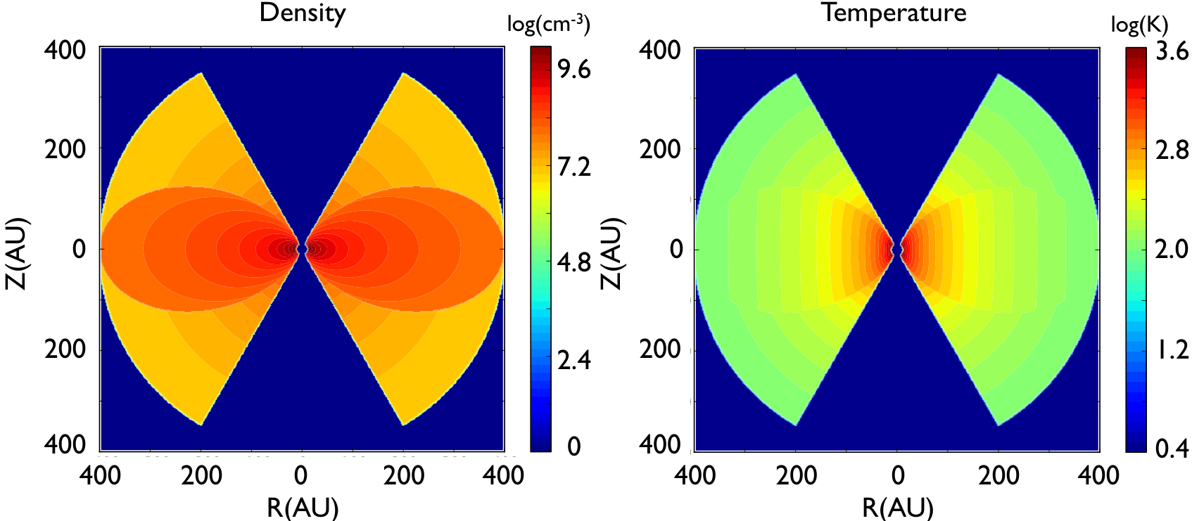
To explore if a kinematical model as suggested in the previous section can reproduce the observed velocity pattern and molecular line spectra, we constructed a toy model and calculate the resulting emission using the axisymmetric radiative transfer code RATRAN (Hogerheijde & van der Tak 2000). Our model includes a flattened “disk-like” structure surrounded by a static spherical envelope and a bipolar outflow cavity (Fig. 10). We adopt a parametrized description of the density, temperature, and velocity field, and assume LTE and optically thin conditions for the line emission. Given the critical densities of the observed transitions (, and cm-3 for HDO, H218O and SO2 at 200 K, respectively), and the densities derived in Sect. 3.1.2, the excitation is likely in LTE. We scale the model intensity to match the observed line strengths, which means that we can derive conclusions about the velocity field but not the density or temperature. Our only aim is to show that our simple toy model can reproduce the observed velocity pattern and spectral line shapes. We do not perform any global model optimization in density, temperature and velocity profiles. Instead, for fixed sets of density and temperature profiles, we conduct a simplified optimization to the parametrized velocity field. Our derived parameters are therefore not best-fit solutions but rather indicative values.

4.3 Details of the model
The density profiles for the disk-like structure (for simplicity, we use “disk” hereafter in this section) and the envelope are assumed to follow power-law distributions, respectively, as and , where is the density at radius (the outer radius of the disk), is the disk-to-envelope density ratio at in the mid-plane, is the angle measured from the polar axis, is the flattening parameter and is the power-law index. In the disk density profile, regions with densities lower than are set to have zero density, resulting in a dumpling-like, flattened structure. The overall density in the model is the sum of and . For the temperature profiles in the disk and the envelope, we assume power-law distributions, respectively, as and (i.e., we adopt a vertically isothermal model for the disk) where denotes the radial direction in cylindrical coordinates, is the temperature at , is the disk-to-envelope temperature ratio, and is the power-law index. The gas temperature for a given position is the weighted mean of the disk and envelope values: . The distance to the source is assumed to be 1 kpc. The inner radius of the model is set to 12.5 AU (van der Tak & Menten 2005, half the size of the HII region;) and the outer radius to 400 AU (, based on the size derived from our 203.4 GHz continuum). In addition, a bipolar outflow cone with an opening angle of is included in the model by setting the density inside this cone to be zero. We describe the velocity field in the disk by three orthogonal components as radial (), vertical () and azimuthal (). The velocity field in the static envelope is set to be purely turbulent, inspired by the observed spectra showing emission peaks near systemic velocity. The gas velocity for a given position is the weighted mean of the disk and envelope values: . The inclination of the source is set to be (van der Tak et al. 2006) with the blue-shifted outflow cone pointed to the west. Model parameters are chosen to ensure that the LTE and optically thin assumptions are valid. We adopt , cm-3, , , , K, , a molecular fractional abundance of and a turbulent line width of 0.5 km s-1. A detailed description of the parametrized velocity field is given in the next section. We scale the line intensity to the observed values, and only analyze the velocity signatures (moment 1 maps and position-velocity maps) and spectral line profiles. We note that this scaling process makes the exact profiles of density and temperature irrelevant.
4.4 Evidence of sub-Keplerian rotation and Hubble-law like radial expansion traced by HDO and H218O
The analysis of the position-velocity maps of the observed lines toward VLA3 reveals that the velocity field is characterized by a linear velocity gradient (Fig. 5), which suggests that the equatorial region is undergoing solid-body rotation. However, the analysis demonstrated in Fig. 9 implies that an extra outward radial component is required to reproduce the observed northeast-southwest velocity pattern (Fig. 3 (d)–(f)). Therefore, a direct link between the observed linear velocity gradient and the inferred solid-body rotation may not be trivial. In our toy model, we consider two types of velocity profiles in the azimuthal and radial directions for the disk-like structure: one is proportional to and the other follows . Although all the combinations of the velocity field can reproduce the triple-peaked line signature seen in HDO and the linear velocity gradient seen in the position-velocity maps, only Keplerian-like rotation () plus Hubble-law like radial expansion () can reproduce the mirrored S-shape isovelocity contours observed in H218O, which is less affected by the outflow than SO2 (Fig. 11; c.f., Fig. 3(e)). An additional velocity component in the direction may redistribute the isovelocity contours to match the observed SO2 moment 1 map. In our toy model, the outflow component is not included due to the complexity of outflow morphology and velocity field. Therefore, we use HDO and H218O data to constrain the kinematics of the equatorial region of VLA3. To summarize, we adopt the parametrized velocity for the disk-like structure as:
| (5) |
where is an analog of the Hubble constant, is a constant between 0 and 1, is the gravitational constant and =16 (van der Tak & Menten 2005) is the stellar mass.

To estimate the strength of the two free parameters and in our kinematic model, we perform a simplified parameter optimization which utilizes the peak velocities of the HDO triple-peaked line profile (, and km s-1 for the blue-shifted, systemic and red-shifted components, respectively), and the measured linear velocity gradient of km s-1 arcsec-1 at P.A as the constraints. We constructed a grid of models for HDO with between 4 and 20 km s-1 per 1000 AU and between 0.2 and 0.5. For each set of parameters (, ), we compute , which is smaller for a better match. Figure 12 shows that the models with the lowest values span a diagonal in (, )-space, indicating that the model is degenerate. To break the degeneracy, we compute the strength of the linear velocity gradient at P.A. in our grid model and plot it as the solid curves in Fig. 12. By matching the observed value, we conclude that based on our toy model, the azimuthal motion of the disk-like structure traced by HDO can be characterized by sub-Keplerian rotation (about 1/3 the strength of Keplerian rotation with a stellar mass of 16 ) and the radial motion is the accelerated expansion with the analogue Hubble constant of 10 km s-1 per 1000 AU at 1 kpc. The best matching model spectrum, moment 1 maps and position-velocity map for HDO can be found in Fig. 13 (a)–(e).
To model the H218O data, we use the best matching solution for HDO ( = 10 km s-1 arcsec-1, = 0.35) as the starting point. Certainly, the turbulent line width of 0.5 km s-1 is too narrow for H218O since its line profile is Gaussian-like with hints of secondary velocity components. We therefore adopt a turbulent line width of 1.0 km s-1 in the model. The best matching model for H218O can be seen in Fig. 13 (f)–(j). Though not perfectly matching the observations, our toy model of kinematics is able to reproduce both HDO and H218O data qualitatively. In our toy model, we found that the kinematics of the proposed disk-like structure around VLA3 is best described by two velocity components: sub-Keplerian rotation and Hubble-law like expansion. We also found that the conclusion of rigid-body rotation across the source judging directly from the linear velocity gradient observed in position-velocity maps may not be made if the observed velocity gradient does not align well with the equatorial plane defined by the outflow.
5 Discussion
5.1 An embedded disk-like structure in AFGL 2591–VLA3?
Our (sub)arcsecond PdBI images of HDO, H218O and SO2 reveal a clear velocity gradient in the northeast-southwest direction across the source AFGL 2591–VLA3 (Sect. 3.2.2). Together with the shape of the HDO line profile (Sect. 3.2.3), and the symmetric temperature distribution of the blue- and red-velocity components (Sect. 3.2.4), we propose that the source AFGL 2591–VLA3 is surrounded by a disk-like structure undergoing rotation and expansion. The kinematics of the equatorial region is further characterized as sub-Keplerian rotation plus Hubble-law like expansion as shown by radiative transfer modeling of a toy model (Sect. 4). In the models for HDO, a microturbulent line width of km s-1 matches the triple-peaked line profile, which appears small for the violent environment of massive star-forming regions (Zinnecker & Yorke 2007). On the other hand, a microturbulent line width of 1.0 km s-1 is needed to match the almost single-peaked line profiles seen in H218O. We expect that an even larger turbulent line width is required to model SO2, judging from the observed SO2 spectrum. This suggests that these molecules trace different regions within the disk-like structure.
We hypothesize that the disk-like structure has a layered distribution with HDO close to the mid-plane, H218O in the warm mid-layer and SO2 in the upper disk layers (Fig. 14). In addition, significant emission from all three molecules originates in a static turbulent envelope surrounding the disk-like structure, especially for H218O and SO2 where it dominates the line profiles (Table 8). In the disk-like structure, we find temperatures of about 120–165 K, well above the evaporation temperature of water ice (Fraser et al. 2001). The HDO molecules may be formed on grain surfaces (Tielens 1983; Parise et al. 2005), and released into the gas phase when the disk-like structure is heated by shocks, stellar radiation and winds. Compared to HDO, H218O originates from a more turbulent region at larger height with increased turbulence in the disk-like structure. In this picture, the presence of H218O but absence of HDO in the mid-layer of the disk-like structure could be due to increased local water formation because of warm gas chemistry as opposed to evaporation of deuterated ices formed at low temperature. SO2 is a good shock/outflow tracer in massive star-forming regions (Schilke et al. 1997). Judging from the facts that the observed SO2 line profile has significant emission from line wings, and that a relatively large velocity gradient is measured in SO2 compared to HDO/H218O, we suggest that SO2 traces a part of the disk-like structure where the outflow interacts with the upper layers. The concentric velocity patterns seen both in the blue- and red-shifted part of moment 1 maps of SO2 (Fig. 3(i) and (l)) likely support the idea since the most extreme velocities occur in the region close to the star (unlike HDO and H218O) as expected for an outflow origin.
5.2 Kinematics of the proposed disk-like structure and comparison to other disk sources
Our toy model suggests that the proposed disk-like structure around VLA3 undergoes sub-Keplerian rotation which cannot be directly inferred from the observed position-velocity maps. We speculate that a magnetic field slows the rotation down below pure Keplerian, which may help to transport the angular momentum outward in VLA3. Similar to the formation of low-mass stars, the magnetic field has been suggested to play an important role in the formation of high-mass stars as well (Girart et al. 2009; Beuther et al. 2010). In strongly magnetized clouds during collapse, magnetic braking is thought to regulate the formation of disks around stars (Basu & Mouschovias 1994; Allen et al. 2003; Mellon & Li 2008, e.g.,). Certainly in our case, the magnetic field does not fully dominate the kinematics of VLA3, otherwise a solid-body like velocity field would be expected in the inner region of the disk-like structure (c.f. Galli et al. 2006, Fig. 2). From OH maser observations, Hutawarakorn & Cohen (2005) measure a maser disk with radius about 750 AU and the magnetic field strength of a few mG toward AFGL 2591–VLA3, which may be sufficient to slow down the rotation. Subarcsecond dust polarization measurements of the magnetic field toward VLA3 and hence deriving the mass-to-flux ratio would be helpful to test our hypothesis if the magnetic field indeed regulates the kinematics of the equatorial regions of young high-mass stars.
In addition to sub-Keplerian rotation, we found that Hubble-law like expansion occurs in the equatorial region of VLA3. The overall kinematics is similar to the SiO maser disk around Orion–IRc2 in which Keplerian rotation and decelerated expansion characterize the kinematics (Plambeck et al. 1990). The expanding motions in the disk could be due to the interaction between the stellar radiation and winds with the disk-like structure, providing the forces to push the gas outward (Hollenbach et al. 1994; Yorke & Welz 1996; Richling & Yorke 1997, e.g.,). On the other hand, the presence of an expanding velocity component in the disk-like structure could be the result of accretion through the mid-plane of the very inner region so that the expansion helps to conserve the angular momentum in the equatorial region. The infrared speckle imaging of AFGL 2591 by Preibisch et al. (2003) suggests that the outflow or wind is variable in time thus the accretion in the disk may not be continuous but episodic. In addition, little free-free emission is detected toward the source, indicating an evolutionary stage before the development of an ultracompact HII region (van der Tak & Menten 2005). As a result, the main accretion phase might have ceased although models show that massive young stars can continue to gain mass through the disk even after an ultracompact HII region has been developed (Keto 2007, e.g.,). Future high-resolution observations of multiple HDO lines and other dense gas tracers, such as N2D+ and CH3CN, would be useful to constrain the physical condition and the kinematics of the disk-like structure around VLA3 better and understand its evolutionary stage of high-mass star formation.
Although massive disks showing pure Keplerian rotation traced by various molecules are reported such as the cases in IRAS 20126+4104 (Cesaroni et al. 2005, C34S;), AFGL 490 (Schreyer et al. 2006, C17O;) and NGC 7538S (Sandell et al. 2003, H13CN;), cases showing non-Keplerian rotation were observed as well such as AFGL 2591 (HDO, H218O; this work) and IRAS 18089$-$1732 (Beuther & Walsh 2008, NH3;). In addition, massive disk candidates have a wide range of mass and size distributions derived via various tracers as summarized by Cesaroni et al. (2007). Despite the fact that the detections of massive disks to date are still limited, Keplerian rotation in the disks is typically found toward young massive stars with masses about 10 such as the cases quoted above. For stellar masses about 16 , massive disks start to show non-Keplerian motion such as rigid-body rotation reported in the literature. For even higher stellar masses, the rotating structures (toroids) typically show solid-body rotation and are gravitationally unstable (Beltrán et al. 2005; Furuya et al. 2008). The sub-Keplerian rotation discovered in our work suggests that AFGL 2591–VLA3 may be a special case linking transition of velocity field of massive disks from pure Keplerian rotation to solid-body rotation though definitely more new detections of circumstellar disks around high-mass YSOs are required to examine this hypothesis.
5.3 Effect of the uncertainty in distance
The distance to AFGL 2591 is uncertain as discussed by van der Tak et al. (1999) and Rygl et al. (2011). In this paper, we assume a distance of 1 kpc with total luminosity of 20000 . From the radiative transfer modeling of HDO/H218O with our toy model, we found that the azimuthal motion of the proposed disk-like structure is dominated by sub-Keplerian rotation which is about 1/3 in strength of pure Keplerian rotation with a stellar mass of 16 , and the radial motion is consistent with Hubble-law like expansion with the analogue Hubble constant of 10 km s-1 arcsec-1. For other distances, our results remain unchanged except for the relative strengths of rotation and expansion. In particular, scales as and scales as , so that for and 3.0 kpc, is changed to 20 and 3.3 km s-1 arcsec-1, while becomes 0.5 (effective Keplerian mass = 4 ) and 0.2 (effective Keplerian mass = 0.7 ). We suggest that the disk-like structure cannot undergo pure Keplerian rotation at any of these distances since the effective Keplerian masses are not consistent with the scaled total luminosities.
6 Conclusions
Our (sub)arcsecond resolution PdBI observations in millimeter continuum and in lines of HDO 11,0–11,1, H218O – and SO2 – successfully resolve the inner thousand AU region of the young high-mass star AFGL 2591–VLA3. We summarize our findings below.
- 1.
From the visibility analysis of millimeter continuum and molecular lines, a compact source with diameter of AU at 1 kpc is found toward VLA3. Depending on the assumptions, the H2 column density, number density and mass are estimated to be cm-2, cm-3 and 0.2 , respectively.
- 2.
A linear velocity gradient in the northeast-southwest direction is found across the source, which has an offset in P.A. by to the equatorial region (P.A. ) defined by the east-west outflow. We interpret this kinematical signature as a combination of rotation and radial expansion in the equatorial region of VLA3.
- 3.
By introducing a toy model with simplified parameter optimization, we further constrain the rotation to be sub-Keplerian and the radial expansion to be Hubble-law like. This result is independent to the distance of the source.
- 4.
We speculate that sub-Keplerian rotation in the equatorial region could be effect of magnetic field which turns the velocity profile from pure Keplerian to sub-Keplerian. The expansion could be due to the interaction between the stellar radiation/winds and the gas in the equatorial region of VLA3.
- 5.
Based on the molecular line profiles, the chemical structure of the proposed disk appears layered, with HDO near the mid-plane, H218O in the mid-layer and SO2 in the upper layers, judging from their turbulent line widths.
Acknowledgements.
The authors appreciate the anonymous referee for the critical comments which help the preparation of the manuscript. The authors are also grateful to the staff of the Plateau de Bure telescope for assisting with the observations, especially Jan Martin Winters at IRAM Grenoble. The research of K.-S.W. at Leiden Observatory is supported through a Nederlandse Onderzoekschool Voor Astronomie (NOVA) Ph.D. grant.References
- Allen et al. (2003) Allen, A., Li, Z., & Shu, F. H. 2003, ApJ, 599, 363
- Armitage (2011) Armitage, P. J. 2011, ARA&A, 49, 195
- Basu & Mouschovias (1994) Basu, S. & Mouschovias, T. C. 1994, ApJ, 432, 720
- Beltrán et al. (2005) Beltrán, M. T., Cesaroni, R., Neri, R., et al. 2005, A&A, 435, 901
- Beuther et al. (2002) Beuther, H., Schilke, P., Sridharan, T. K., et al. 2002, A&A, 383, 892
- Beuther et al. (2010) Beuther, H., Vlemmings, W. H. T., Rao, R., & van der Tak, F. F. S. 2010, ApJ, 724, L113
- Beuther & Walsh (2008) Beuther, H. & Walsh, A. J. 2008, ApJ, 673, L55
- Beuther et al. (2005) Beuther, H., Zhang, Q., Sridharan, T. K., & Chen, Y. 2005, ApJ, 628, 800
- Bruderer et al. (2009) Bruderer, S., Benz, A. O., Bourke, T. L., & Doty, S. D. 2009, A&A, 503, L13
- Campbell (1984) Campbell, B. 1984, ApJ, 287, 334
- Cesaroni et al. (1999) Cesaroni, R., Felli, M., Jenness, T., et al. 1999, A&A, 345, 949
- Cesaroni et al. (1997) Cesaroni, R., Felli, M., Testi, L., Walmsley, C. M., & Olmi, L. 1997, A&A, 325, 725
- Cesaroni et al. (2007) Cesaroni, R., Galli, D., Lodato, G., Walmsley, C. M., & Zhang, Q. 2007, Protostars and Planets V, 197
- Cesaroni et al. (2006) Cesaroni, R., Galli, D., Lodato, G., Walmsley, M., & Zhang, Q. 2006, Nature, 444, 703
- Cesaroni et al. (2005) Cesaroni, R., Neri, R., Olmi, L., et al. 2005, A&A, 434, 1039
- Fraser et al. (2001) Fraser, H. J., Collings, M. P., McCoustra, M. R. S., & Williams, D. A. 2001, MNRAS, 327, 1165
- Furuya et al. (2008) Furuya, R. S., Cesaroni, R., Takahashi, S., et al. 2008, ApJ, 673, 363
- Galli et al. (2006) Galli, D., Lizano, S., Shu, F. H., & Allen, A. 2006, ApJ, 647, 374
- Girart et al. (2009) Girart, J. M., Beltrán, M. T., Zhang, Q., Rao, R., & Estalella, R. 2009, Science, 324, 1408
- Goldsmith & Langer (1999) Goldsmith, P. F. & Langer, W. D. 1999, ApJ, 517, 209
- Hasegawa & Mitchell (1995) Hasegawa, T. I. & Mitchell, G. F. 1995, ApJ, 451, 225
- Henning et al. (2000) Henning, T., Schreyer, K., Launhardt, R., & Burkert, A. 2000, A&A, 353, 211
- Hogerheijde & van der Tak (2000) Hogerheijde, M. R. & van der Tak, F. F. S. 2000, A&A, 362, 697
- Hollenbach et al. (1994) Hollenbach, D., Johnstone, D., Lizano, S., & Shu, F. 1994, ApJ, 428, 654
- Hutawarakorn & Cohen (2005) Hutawarakorn, B. & Cohen, R. J. 2005, MNRAS, 357, 338
- Keto (2007) Keto, E. 2007, ApJ, 666, 976
- Keto & Zhang (2010) Keto, E. & Zhang, Q. 2010, MNRAS, 406, 102
- Krumholz et al. (2009) Krumholz, M. R., Klein, R. I., McKee, C. F., Offner, S. S. R., & Cunningham, A. J. 2009, Science, 323, 754
- Lada et al. (1984) Lada, C. J., Thronson, Jr., H. A., Smith, H. A., Schwartz, P. R., & Glaccum, W. 1984, ApJ, 286, 302
- Mellon & Li (2008) Mellon, R. R. & Li, Z. 2008, ApJ, 681, 1356
- Mitchell et al. (1992) Mitchell, G. F., Hasegawa, T. I., & Schella, J. 1992, ApJ, 386, 604
- Ossenkopf & Henning (1994) Ossenkopf, V. & Henning, T. 1994, A&A, 291, 943
- Parise et al. (2005) Parise, B., Ceccarelli, C., & Maret, S. 2005, A&A, 441, 171
- Plambeck et al. (1990) Plambeck, R. L., Wright, M. C. H., & Carlstrom, J. E. 1990, ApJ, 348, L65
- Preibisch et al. (2003) Preibisch, T., Balega, Y. Y., Schertl, D., & Weigelt, G. 2003, A&A, 412, 735
- Richling & Yorke (1997) Richling, S. & Yorke, H. W. 1997, A&A, 327, 317
- Rygl et al. (2011) Rygl, K. L. J., Brunthaler, A., Sanna, A., et al. 2011, ArXiv e-prints
- Sandell et al. (2003) Sandell, G., Wright, M., & Forster, J. R. 2003, ApJ, 590, L45
- Schilke et al. (1997) Schilke, P., Groesbeck, T. D., Blake, G. A., & Phillips, T. G. 1997, ApJS, 108, 301
- Schreyer et al. (2006) Schreyer, K., Semenov, D., Henning, T., & Forbrich, J. 2006, ApJ, 637, L129
- Shepherd & Kurtz (1999) Shepherd, D. S. & Kurtz, S. E. 1999, ApJ, 523, 690
- Simon et al. (2000) Simon, M., Dutrey, A., & Guilloteau, S. 2000, ApJ, 545, 1034
- Tielens (1983) Tielens, A. G. G. M. 1983, A&A, 119, 177
- Trinidad et al. (2003) Trinidad, M. A., Curiel, S., Cantó, J., et al. 2003, ApJ, 589, 386
- van der Tak & Menten (2005) van der Tak, F. F. S. & Menten, K. M. 2005, A&A, 437, 947
- van der Tak et al. (1999) van der Tak, F. F. S., van Dishoeck, E. F., Evans, II, N. J., Bakker, E. J., & Blake, G. A. 1999, ApJ, 522, 991
- van der Tak et al. (2006) van der Tak, F. F. S., Walmsley, C. M., Herpin, F., & Ceccarelli, C. 2006, A&A, 447, 1011
- Williams & Cieza (2011) Williams, J. P. & Cieza, L. A. 2011, ARA&A, 49, 67
- Wilson & Rood (1994) Wilson, T. L. & Rood, R. 1994, ARA&A, 32, 191
- Yorke & Welz (1996) Yorke, H. W. & Welz, A. 1996, A&A, 315, 555
- Zhang et al. (2005) Zhang, Q., Hunter, T. R., Brand, J., et al. 2005, ApJ, 625, 864
- Zinnecker & Yorke (2007) Zinnecker, H. & Yorke, H. W. 2007, ARA&A, 45, 481