Effective electron recombination coefficient in ionospheric D-region during the relaxation regime after solar flare from February 18, 2011
Abstract
In this paper, we present a model for determination of a weakly time dependent effective recombination coefficient for the perturbed terrestrial ionospheric D-region plasma. We study consequences of a class M1.0 X-ray solar flare, recorded by GOES-15 satellite on February 18, 2011 between 14:00 UT and 14:15 UT, by analyzing the amplitude and phase real time variations of very low frequency (VLF) radio waves emitted by transmitter DHO (located in Germany) at frequency 23.4 kHz and recorded by the AWESOME receiver in Belgrade (Serbia). Our analysis is limited to ionospheric perturbations localized at altitudes around 70 km where the dominant electron gain and electron loss processes are the photo-ionization and recombination respectively.
Keywords:
electron concentration, photo-ionization, electron recombination, solar flare, ionospherePACS
94.20.de , 94.20.Vv , 94.20.Fg , 96.60.qe1 Introduction
The ionosphere, having characteristics of plasma, is very sensitive to electromagnetic disturbances whose intensity and number vary with solar activity. These disturbances cause numerous complicated physical, chemical and dynamical phenomena in the lower ionosphere and may directly affect human activities, especially in the telecommunications industry. Besides a pure scientific interest to study the influence of solar activity on the terrestrial atmosphere, the understanding and predicting the resulting turbulent regions of the ionosphere has important applications for radio communications, military operations in remote locations, planned networks of mobile communications satellites, high-precision applications of global navigation satellite systems, etc.
The VLF radio signal propagation properties are determined by the wave attenuation and reflection which depend on the electron concentration and collision frequency. The electron concentration calculations in empirical and semi-empirical models are based mainly on measurements using radio-wave propagation methods and sounding rockets.
Due to a varying complex structure of the atmosphere and because of numerous influences coming from the Earth and outer space, experimental simulations of processes in the ionosphere are very difficult. For this reason, theoretical models are of a basic importance in providing us with information on ionospheric parameters, with the effective recombination coefficient being one of them. This coefficient plays an important role in the ionization balance and in kinetics of underlying chemical reactions and from its values one can estimate the structure of the lower ionosphere.
In the Earth ionosphere, the electron concentration depends on photo-ionization and recombination processes. At heights around 70 km, the dominant recombination processes are the electron-ion, ion-ion and three-body recombination characterized by a common effective recombination coefficient [1].
In the case of unperturbed, quasi-stationary ionosphere, the electron gain and electron loss processes are in equilibrium, i.e. mutually balanced.
During a solar flare, the electron concentration is raised due to increased photo-ionization and this time period can be named as photo-ionization regime. After a flare maximum when the rate of recombination becomes larger than the photo-ionization rate, the electron concentration starts to decrease and the ionosphere enters a recombination regime.
In this paper, we calculate the time dependence of effective recombination coefficient for different altitudes in the ionospheric D-region for the tail of the recombination regime. The considered class M1.0 X-ray solar flare was recorded by GOES-15 satellite on February 18, 2011 between 14:00 and 14:15 UT. Our analysis uses a discrete set of data on amplitude and phase variations of the 23.4 kHz VLF signal emitted by the transmitter DHO in Germany and registered by the AWESOME 11 1 Atmospheric Weather Electromagnetic System for Observation Modeling and Education. receiver system [2] in Belgrade22 2 A part of Stanford/AWESOME Collaboration for Global VLF Research., Serbia with the sampling period of 0.02 s. These experimental data were treated by the LWPC (Long-Wave Propagation Capability) computer program [3] for modeling the ionosphere which yielded discrete sets of data on the wave reflection heights and sharpness the basic parameters of Wait′s model of the ionosphere [4] needed to compute the distribution profiles of electron concentration and the effective recombination coefficient where is the location altitude.
2 Basic theory
The electron concentration at altitude in the D-region is time dependent and is taken to obey the following differential equation [5]:
| (1) |
where the concentrations of negative ions and their time derivatives are comparatively small at altitudes of about 70 km [6] so that their contributions are not taken into account.
According to the Chapman′s theory [7] the rate of electron production can be expressed as:
| (2) |
where is the X-ray radiation flux intensity and is a proportionality coefficient whose explicit expression turns out not to be required in our computations.
The X-ray radiation flux intensity at some level is related to its value (measured by the satellite GOES-15) through the following relation:
| (3) |
where , like in Eq. (2), is a proportionality coefficient whose explicit expression will not be needed in our further treatment.
| (4) |
with the coefficient given by:
| (5) |
After a sufficient time interval following the intensity maximum (the shaded domain in Fig. 1), the coefficients and become weakly time dependent and we will consider them approximately constant within some finite time interval :
Eq. (4) can now be applied to the interval end points and which yields the following set of two algebraic equations for unknown quantities and :
| (6) |
which finally gives the expression for numerical computation of the weakly time dependent effective recombination coefficient :
| (7) |
where:
| (8) |
3 Experimental data and calculation procedure
Within the time interval 14:00 UT - 14:15 UT, February 18, 2011, a solar flux increase was registered in the range 0.1-0.8 nm by the GOES-15 satellite whose maximal value corresponded to the level typical of a class M1.0 solar X flare (Fig. 1). This rise on the radiation flux altered the rate of photo-ionization and electron recombination process and, consequently, it changed the electron concentration. As a result, the recorded VLF wave exhibits a time varying amplitude and phase as shown in Fig. 1.
To obtain the effective recombination coefficient profiles given by Eqs. (7)-(9) we need the explicit expression for the time dependence of the electron concentration profile and its time derivative as well as the incoming solar radiation flux as recorded by the GOES-15 satellite.
The electron concentration is computed by the following relation [4]:
| (9) |
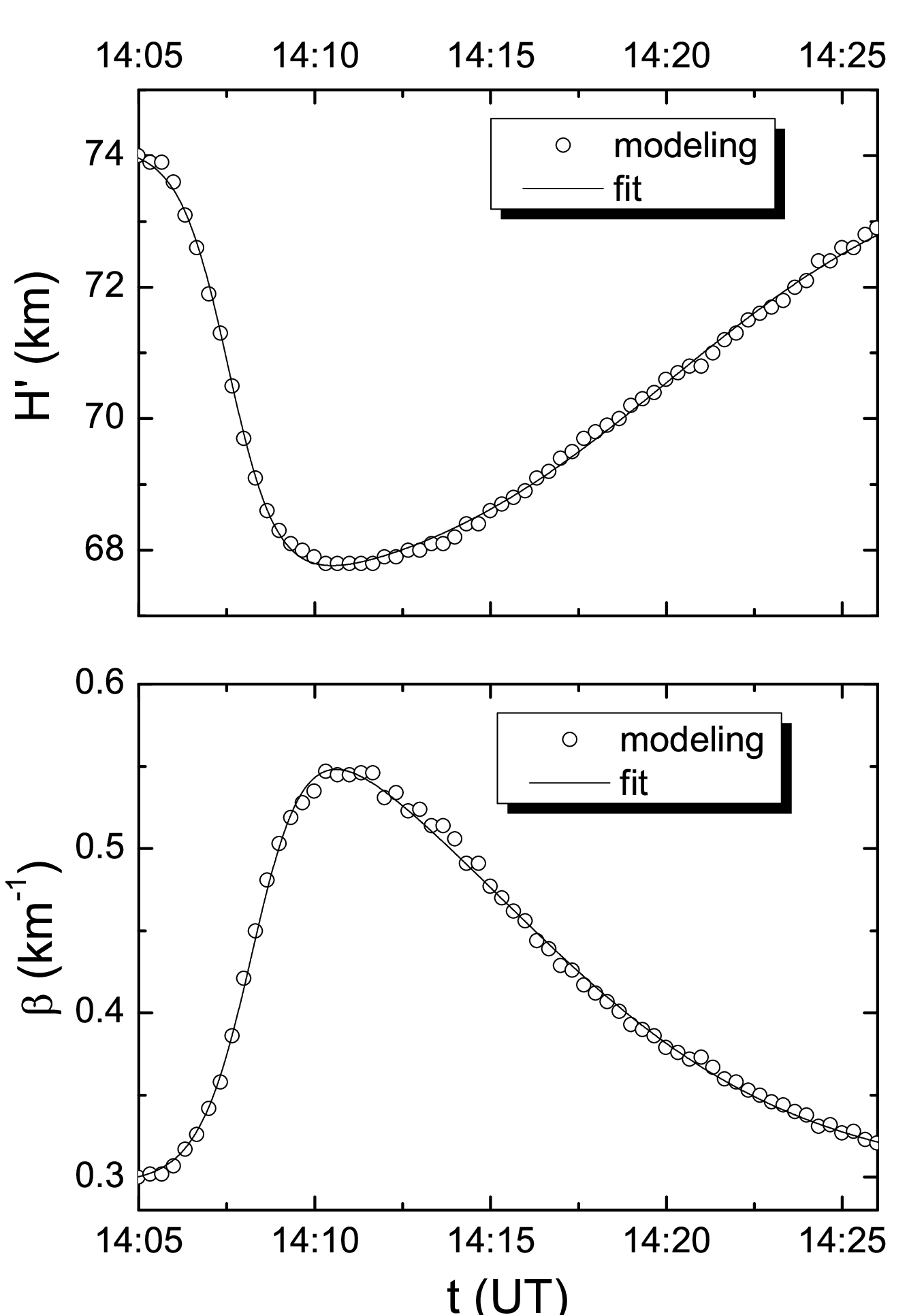
where and are defined as the wave reflection height and sharpness respectively. Quantities and are determined by the LWPC computer program [3] using the recorded discrete time-set of values for the amplitude and phase of the considered VLF 23.4 kHz VLF signal ([8, 9]). Time dependencies of these two parameters are shown in Fig. 2 where it can be seen that the VLF wave reflection height initially decreases in time and reaches a minimum at about two minutes after the solar flux maximum (Fig. 2). The sharpness , characterizing the gradient of the electron concentration with height, has a reversed time distribution, i.e. it first increases and attains a maximum at the same time when has its minimum.
As the recorded quantities are discrete in time, the input radiation flux intensity and the derived values for and are not smooth functions of time and we fitted them by a continuous model function implemented in the Origin-8 program, also found in the NAG (Numerical Algorithms Group) library:
| (10) |
where is time in seconds starting from 14:04:00 UT and stands for , , and . The numerical fitting constants , , , , and related to the considered physical quantities in Eq. (10) were obtained as the program outputs and are presented in Table 1.
4 Results and discussion
The electron concentrations at various heights and their time derivatives obtained from Eq. (9) are shown in Figs 3 and 4 respectively. We can see that the considered solar flare causes larger increases in electron concentration at higher altitudes. Comparing Fig. 1 and Fig. 3 it can be noticed that the time distribution of the electron concentration follows the time variation pattern of the registered solar flux on GOES-15 satellite. Maximum of solar flux occurs at 11:24 UT which is about two minutes before the time when the corresponding maximum appears in the electron concentration curve. At considered altitudes of around 70 km, the dominant electron gain and electron loss processes are the photo-ionization and recombination respectively. Within the time period before the electron concentration maximum, the rate of the photo-ionization is larger then that of recombination processes. Contrary, the domination of recombination processes causes a decreasing electron concentration as seen in the recombination regime in Fig. 3.
The rate of the electron concentration change is more pronounced at higher altitudes. It is positive when photo-ionization processes dominate the recombination processes. Contrary, the domination of the recombination produces a time decrease of the electron concentration and, consequently, its negative time derivative.
In Fig. 1, the shaded time domain indicates a relatively slow time variation of indicated quantities that allows us to use the procedure for calculation effective recombination coefficient according to the described basic theory. Time variations of are presented in Fig. 5 for different altitudes. Unlike the electron concentration, the effective recombination coefficient has larger values at smaller altitudes.
The increase of coefficient is in agreement with [1] where has larger values for smaller maxima of flare radiation intensity.
5 Conclusion
In this work, we present a method to calculate the effective recombination coefficient at altitudes around 70 km for the tail of the recombination regime. It is shown that the effective recombination coefficient depends on the solar flux intensity, electron concentration and its time derivative. We present a method of determining the electron concentration by comparing the recorded VLF signal amplitude and phase changes with the corresponding values obtained numerically using the LWPC computer program. In the case of this flare, the effective recombination coefficient has values within the order of magnitude to .
Acknowledgment
The present work has been performed under the Ministry of Education and Science of the Republic of Serbia (projects III 44002, 176002 and 176004), Slovenian Research Agency, contract P2-0056 and Joint Bilateral project: BI-SLO-SR.
References
- [1] V. Žigman, D. Grubor & D. Šulić, J. Atmos. Sol.-Terr. Phy. 69, 775-792 (2007).
- [2] D. Scherrer, M. Cohen, T. Hoeksema, U. Inan, R. Mitchell & P. Scherrer, Adv. Space. Res. 42, 1777 (2008).
- [3] J.A. Ferguson, Computer Programs for Assessment of Long-Wavelength Radio Communications, Version 2.0, Space and Naval Warfare Systems Center, San Diego, CA, (1998).
- [4] J.R. Wait & K.P. Spies, Characteristics of the Earthionosphere waveguide for VLF radio waves, NBS Technical Note, 300, Colorado (1964).
- [5] E.V. Appleton, J. Atmos. Terr. Phys. 3, 282 (1953).
- [6] H. Rishbeth & O.K. Garriott, Introduction to Ionospheric Physics, Academic Press, New York, London (1969).
- [7] S. Chapman, Proc. Phys. Soc. 43, 26 (1931).
- [8] D.P. Grubor, D.M. Šulić & V. Žigman, Ann. Geophys. 26, 1731 (2008).
- [9]
D. Šulic, A. Nina & V. Sreckovic, Pub. Astro. Obs. Belgr. 89, 391 (2010).
| 2.07417E-6 | 1.97397E-5 | 196.87571 | 7.05136E-37 | 29.81728 | 282.37906 | |
| (W/m | W/m2 | W/m2 | s | s | s | s |
| 0.29789 | 0.33295 | 0.59163 | 0.0051 | 5.05997E-4 | 0.00278 | |
| (km | km-1 | km-1 | s | s | s | s |
| 74.13507 | -7.06355 | 590.67954 | 754.49827 | 41.86687 | 242.7825 | |
| (km) | km | km | s | s | s | s |