Universality of modulation length (and time) exponents

Saurish Chakrabarty Affiliation: Department of Physics and Center for Materials Innovation, Washington University in St Louis, MO 63130, USA. Vladimir Dobrosavljević Affiliation: Department of Physics and National High Magnetic Field Laboratory, Florida State University, Tallahassee, Florida 32306, USA. Alexander Seidel Affiliation: Department of Physics and Center for Materials Innovation, Washington University in St Louis, MO 63130, USA. Zohar Nussinov Email: zohar@wuphys.wustl.edu Affiliation: Department of Physics and Center for Materials Innovation, Washington University in St Louis, MO 63130, USA. Affiliation: Kavli Institute for Theoretical Physics, Santa Barbara, CA 93106.

August 24, 2026

Abstract

We study systems with a crossover parameter $\lambda$ , such as the temperature $T$ , which has a threshold value $\lambda_{*}$ across which the correlation function changes from exhibiting fixed wavelength (or time period) modulations to continuously varying modulation lengths (or times). We report on a new exponent, $\nu_{L}$ , characterizing the universal nature of this crossover. These exponents, similar to standard correlation length exponents, are obtained from motion of the poles of the momentum (or frequency) space correlation functions in the complex $k$ -plane (or $\omega$ -plane) as the parameter $\lambda$ is varied. Near the crossover (i.e., for $\lambda\to\lambda_{*}$ ), the characteristic modulation wave-vector $K_{R}$ on the variable modulation length “phase” is related to that on the fixed modulation length side, $q$ via $|K_{R}-q|\propto|T-T_{*}|^{\nu_{L}}$ . We find, in general, that $\nu_{L}=1/2$ . In some special instances, $\nu_{L}$ may attain other rational values. We extend this result to general problems in which the eigenvalue of an operator or a pole characterizing general response functions may attain a constant real (or imaginary) part beyond a particular threshold value, $\lambda_{*}$ . We discuss extensions of this result to multiple other arenas. These include the axial next nearest neighbor Ising (ANNNI) model. By extending our considerations, we comment on relations pertaining not only to the modulation lengths (or times) but also to the standard correlation lengths (or times). We introduce the notion of a Josephson timescale. We comment on the presence of aperiodic “chaotic” modulations in “soft-spin” and other systems. These relate to glass type features. We discuss applications to Fermi systems – with particular application to metal to band insulator transitions, change of Fermi surface topology, divergent effective masses, Dirac systems, and topological insulators. Both regular periodic and glassy (and spatially chaotic behavior) may be found in strongly correlated electronic systems.

pacs

05.50.+q, 75.10.Hk, 75.60.Ch

I Introduction

In complex systems, there are, in general, possibly many important length and time scales that characterize correlations. Aside from correlation lengths describing the exponential decay of correlations, in some materials there are length scales that characterize periodic spatial modulations or other spatially non-uniform properties as in Fig. 1.

Refer to caption — Figure 1: Sub-unit-cell resolution image of the electronic structure of a cuprate superconductor at the pseudo-gap energy. Inset shows Fourier space image of the same figure. Nematic and smectic phases are highlighted using the red and blue circles respectively. The nematic phase is characterized by commensurate wave-vectors $\vec{Q}$ . The smectic wave-vector, on the other hand takes incommensurate values, $\vec{S}$ which is dependent on the amount of doping, albeit weakly. (From Ref. [1]. Reprinted with permission from AAAS.)

We investigate the evolution of these length scales as a function of some parameter $\lambda$ . This parameter may be the temperature, the chemical potential, or some other physical quantity relevant for description of the system being studied. To illustrate our basic premise, we will largely focus on temperature dependences of the correlation function in this work. However, with a trivial change of variables, our results are valid for any parameter that, when tuned, connects a phase with continuously varying modulation lengths (or times) to one in which the modulation length (or time) is pinned to a fixed value. The crossovers we consider are not symmetry breaking transitions. Consequences of our considerations also relate to correlation lengths as we will comment on later.

Many systems exhibit subtle changes in their correlation functions at certain special temperatures. We focus on situations wherein as the temperature is varied across a certain crossover temperature $T_{*}$ , an unmodulated phase of a system (appearing at $T>T_{*}$ or at $T<T_{*}$ ) may start exhibiting modulations (at $T<T_{*}$ or at $T>T_{*}$ respectively) sans a thermodynamic phase transition at $T_{*}$ . A generalization of this occurs when modulations in a system are characterized by a fixed wavelength on one side of a crossover temperature and by continuously varying wavelengths on the other side. Such an occurrence may generally rear its head when interactions of different scales compete with one another. A wealth of interesting periodic spatial patters appear arenas: e.g., the manganites,[2] pnictide [3, 4] and cuprate [5, 6, 7, 8, 9, 10] superconductors, quantum Hall systems,[11, 12, 13] dense nuclear matter,[14, 15] magnetic systems,[16, 17, 18, 19, 20, 21] heavy fermion compounds,[22, 23] membranes,[24] cholesterols,[25] magnetic garnets,[26] dipolar systems,[27, 28] systems with nematic phases,[29] and countless other systems.[30, 31, 32, 33, 34]

II Our main results and their implications

In this work, we report on the temperature (or other parameter) dependence of emergent modulation lengths that govern the size of various domains present in some systems. In its simplest incarnation, our central result is that if fixed wavelength modulations characterized by a particular finite length scale, $L_{*}$ , appear beyond some temperature $T_{*}$ then, the modulation length, $L_{D}$ on the other side of the crossover differs from $L_{*}$ as

\displaystyle|L_{D}-L_{*}|\propto|T-T_{*}|^{\nu_{L}}.

(1)

When there are no modulations on one side of $T_{*}$ , i.e., $L_{*}\to\infty$ , we have near the crossover,

\displaystyle L_{D}\propto|T-T_{*}|^{-\nu_{L}}.

(2)

Apart from some special situations, we find that irrespective of the interaction, $\nu_{L}=1/2$ . We arrive at this rather universal result assuming that there is no phase transition at the crossover temperature $T_{*}$ . Our result holds everywhere inside a given thermodynamic phase of a system.

Our considerations are not limited to continuous crossovers. A corollary of our analysis pertains to systems with discontinuous (“first-order” like) jumps in the correlation or modulation lengths.

We will further comment on situations in which wherein a branch point appears at $T_{*}$ . We will present examples where we obtain rational and irrational exponents and also the anomalous critical exponent $\eta$ . Our analysis affords general connections to the critical scaling of correlation lengths in critical phenomena.

Our results for length scales can be extended to timescales. We will, amongst other notions, in employing a formal interchange of spatial with temporal coordinates, introduce the concept of a Josephson timescale.

Lastly, further deepening the analogy between results in the spatial and time domain, we will comment on the presence of phases with aperiodic spatial “chaotic” modulations (characteristic of amorphous configurations) in systems governed by non-linear Euler-Lagrange equations. Aperiodic “chaotic” modulations may appear in strongly correlated electronic systems.

In the appendix, we present applications to Fermi systems pertaining to metal–band insulator transition, change of Fermi surface topology, divergence of effective masses, Dirac systems and topological insulators.

III The systems of study

In this work, we will predominantly consider translationally invariant systems on a lattice whose Hamiltonian is given by

\displaystyle H=\frac{1}{2}\sum_{\vec{x}\neq\vec{y}}V(|\vec{x}-\vec{y}|)S(\vec{x})S(\vec{y}).

(3)

The quantities $\{S(\vec{x})\}$ portray classical scalar spins or fields. The sites $\vec{x}$ and $\vec{y}$ lie on a $d$ -dimensional hyper-cubic (or some other) lattice with $N$ sites. We will set the lattice constant to unity. [In the quantum arena, we replace the spins $\vec{S}(\vec{x})$ in Eq. (3) by Fermi or Bose or quantum spin operators.]

The results that will be derived in this work apply to a variety of systems. These include theories with trivial $n$ -component generalizations of Eq. (3). In the bulk of this work, the Hamiltonian has a bilinear form in the spins. We will however, later on, study “soft” spin model with explicit finite quartic terms as we now expand on. An $n$ -component generalization of Eq. (3) is given by the Hamiltonian

	$\displaystyle H$	$\displaystyle=$	$\displaystyle\frac{1}{2}\sum_{\vec{x}\neq\vec{y}}V(\|\vec{x}-\vec{y}\|)\vec{S}(\vec{x})\cdot\vec{S}(\vec{y})+$		(4)
			$\displaystyle\frac{u}{4}\sum_{\vec{x}}\left(\vec{S}(\vec{x})\cdot\vec{S}(\vec{x})-n\right)^{2}.$		(4)

Such a Hamiltonian represents standard (or “hard”) spin or $O(n)$ systems if $u\gg 1$ in the large $u$ limit, the quartic term enforces a “hard” normalization constraint of the particular form $\vec{S}(\vec{x})\cdot\vec{S}(\vec{x})=n$ . For finite (or small) $u$ , Equation (4) describes “soft”-spin systems wherein the normalization constraint is not strictly enforced.

In what follows, $v(k)$ and $s(\vec{k})$ will denote the Fourier transforms of $V(|\vec{x}-\vec{y}|)$ and $S(\vec{x})$ . We employ the following Fourier conventions,

	$\displaystyle a(\vec{k})$	$\displaystyle=$	$\displaystyle\sum_{\vec{x}}A(\vec{x})e^{i\vec{k}\cdot\vec{x}},$
	$\displaystyle A(\vec{x})$	$\displaystyle=$	$\displaystyle\frac{1}{N}\sum_{\vec{k}}a(\vec{k})e^{-i\vec{k}\cdot\vec{x}}.$		(5)

With these conventions in tow, in Fourier space, Eq. (3) reads

\displaystyle H=\frac{1}{2N}\sum_{\vec{k}}v(k)|s(\vec{k})|^{2}.

(6)

When $v(\vec{k})$ is analytic in all momentum space coordinates, it is a function of $|\vec{k}|^{2}=k^{2}$ (and not a general function of $k\equiv\sqrt{\sum_{l=1}^{d}k_{l}^{2}}$ with $\{k_{l}\}$ being the Cartesian components of $\vec{k}$ ). This is so as $|\vec{k}|$ has branch cuts when viewed as a function of a particular $k_{l}$ (with all other $k_{l^{\prime}\neq l}$ held fixed). The lattice Laplacian that links nearest neighbors sites in real space becomes

\displaystyle\Delta_{\vec{k}}=2(\sum_{l=1}^{d}(1-\cos k_{l})

(7)

in $k$ -space. $\Delta_{\vec{k}}$ veers towards $|\vec{k}|^{2}$ in the continuum (small $k$ ) limit. The two point correlation function for the system in Eq. (3) is, $G(\vec{x})=\langle S(0)S(\vec{x})\rangle.$ At large distances $x=|\vec{x}|$ , the correlation function has a general asymptotic behavior

\displaystyle G(x)\approx\sum_{i}f_{i}(x)\cos\left(\frac{2\pi x}{L_{D}^{(i)}}\right)e^{-x/\xi_{i}}.

(8)

In the $i$ -th term, $f_{i}(x)$ is an algebraic prefactor, $L_{D}^{(i)}$ is the modulation length and $\xi_{i}$ is the corresponding correlation length. In general, the function $f_{i}(x)$ may contain a factor with an anomalous exponent $\eta$ (usually not an integer), such as, $f_{i}(x)\propto 1/x^{d-2+\eta}$ . Generally, there can be multiple correlation and modulation lengths. In Fourier space, $G(\vec{k})=\frac{1}{N}\langle|s(\vec{k})|^{2}\rangle.$ The modulation and correlation lengths can be obtained respectively from the real and imaginary parts of the poles of $G(\vec{k})$ in the complex $k$ -plane.

General considerations: Correlation and modulation lengths from momentum space correlation function

The correlation function $G(\vec{x})$ in ( $d$ -dimensional) real space is related to the momentum space correlation function $G(\vec{k})$ by

\displaystyle G(\vec{x})=\int\frac{d^{d}k}{(2\pi)^{d}}G(\vec{k})e^{-i\vec{k}\cdot\vec{x}}.

(9)

On the lattice, the integral above must be replaced by summation over $\vec{k}$ -values belonging to the first Brillouin zone. In the continuum, which we discuss here, the integral range is unbounded. Even in lattice systems, doing an unbounded summation over $\vec{k}$ -values provides a good approximation for the correlation function in real space in many scenarios.

For spherically symmetric problems, i.e., when $G(\vec{k})=G(k)$ ,

\displaystyle G(x)

\displaystyle=

\displaystyle\int_{0}^{\infty}\frac{k^{d-1}dk}{(2\pi)^{d/2}}\frac{\mbox{J}_{d/2-1}(kx)}{(kx)^{d/2-1}}G(k),

(10)

where J ${}_{\nu}(x)$ is a Bessel function of order $\nu$ . The above integral can be evaluated by choosing an appropriate contour in the complex $k$ -plane. The contour can be closed along a circular arc of radius $R\to\infty$ provided

\displaystyle|G(k)|\lesssim k^{-\frac{d+1}{2}},\mbox{ as }k\to\infty.

(11)

In evaluating the integral in Eq. (10), we obtain contributions from residues associated with the poles of the integrand as well as contributions from its branch points. We use $K=K_{R}+iK_{I}$ to represent the poles and branch points of the integrand in the complex plane. The correlation and modulation lengths in the system are determined respectively by the imaginary ( $K_{I}$ ) and real parts ( $K_{R}$ ) of these poles and branch points. Together, all these singularities can be compactly expressed as

\displaystyle\boxed{\frac{1}{G^{(m)}(K)}=0},

(12)

where $0\leq m<\infty$ is the order of the smallest order derivative of $G(k)$ which diverges at $k=K$ .[35]

In footnote [36], we comment on the situation in which the function $G(T,k)$ is an entire function of $k$ (i.e., when is $G$ is analytic everywhere).

IV A universal domain length exponent – Details of analysis

We now derive (via various inter-related approaches), our central result – the existence of a new exponent for the domain length in rather general systems with real or complex scalar fields, vectorial (or tensorial) fields of both the discrete (e.g., Potts like) and continuous variants.

We will now consider the situation in which the system exhibits modulations at a fixed wave-vector $q$ for a finite range of temperatures on one side of $T_{*}$ , [viz., (i) $T>T_{*}$ , or, (ii) $T<T_{*}$ ] and starts to exhibit variable wavelength modulations on the other side [(iii) $T<T_{*}$ for (i) and $T>T_{*}$ for (ii)]. A schematic illustrating this is shown in Fig. 2.

In sub-section IV.1, we will assume that the pair correlation function is meromorphic (realized physically by absence of phase transitions) at the crossover point and illustrate how modulation length exponents may appear. In sub-section IV.2, we will comment on the situation where the crossover point may be a branch point of the correlation function.

IV.1 Crossovers at general points in the complex $k$ -plane

In the up and coming, we will assume that the pair correlator, $G(T,k)$ is a meromorphic function of $k$ and $T$ near a crossover point. Our analysis below is exact as long as we do not cross any phase boundaries. Such a case is indeed materialized in the incommensurate-commensurate crossovers in the three-dimensional axial next-nearest-neighbor Ising (ANNNI) model [37, 38] (which is of type (ii) in the classification above). This phenomenon is also seen in the ground state phase diagram of Frenkel-Kontorova models [39] in which one of the coupling constants is tuned instead of temperature.

In the following, we present two alternative derivations for the universal exponent characterizing this crossover.

IV.1.1 First approach

In general, if the pair correlation function $G(T,k)$ is a meromorphic function of the temperature $T$ and the wave-vector $k$ near a crossover point $(T_{*}k_{*})$ , then $G^{-1}(T,k)$ must have a Taylor series expansion about that point. We have,

\displaystyle G^{-1}(T,k)=\sum_{m_{1},m_{2}=0}^{\infty}A_{m_{1}m_{2}}(T-T_{*})^{m_{1}}(k-k_{*})^{m_{2}}.

(13)

Since $G^{-1}(T_{*},k_{*})=0$ , we have, $A_{00}=0$ . Let us try to find the trajectory of the pole $K(T)$ (with $K(T_{*})=k_{*}$ ) of $G(T,k)$ in the complex $k$ -plane as the temperature is varied around $T_{*}$ . Writing down the leading terms of $G^{-1}(T,k)$ , we have, in general,

	$\displaystyle G^{-1}(T,k)$	$\displaystyle\sim$	$\displaystyle\sum_{p=0}^{[m/a]}(T-T_{})^{m-ap}(k-k_{})^{n+bp}+$		(14)
			$\displaystyle~~~~~~~~o((T-T_{})^{m}(k-k_{})^{n}),$		(14)

as $(T,k)\to(T_{*},k_{*})$ with $m,n,a,b$ integers, $m,n\geq 0$ and $a,b\geq 1$ , $[x]$ represents the greatest integer less than or equal to $x$ and $o(x)$ represents terms negligible compared to $x$ . We have,

\displaystyle K(T)\sim k_{*}+C(T-T_{*})^{a/b},

(15)

where $C$ is some constant, yielding $\nu_{L}=a/b$ . By the very definition of $T_{*}$ , on one side of $T_{*}$ [(i) or (ii) above], there exists at least one root [say, $K(T)$ ] of $G^{-1}$ satisfying $K_{R}(T)=q$ , where $q$ is a constant. On the other side [(iii) above], $K_{R}(T)\neq q$ . As such, the function $K(T)$ is non-analytic at $T_{*}$ . The left hand side of Eq. (15) is therefore not analytic at $T=T_{*}$ , implying that the right hand side cannot be analytic. This means that $(a/b)$ cannot be an integer, which in turn implies that $b\geq 2$ . Therefore, in the most common situations we might encounter,

			$\displaystyle G^{-1}(T,k)\sim A(T-T_{})+B(k-k_{})^{2}$		(16)
		$\displaystyle\implies$	$\displaystyle a=1\mbox{ and }b=2.$		(16)

When Fourier transforming $G(T,k)$ by evaluating the integral in Eqs. (9, 10) using the technique of residues, the real part of the poles (i.e., $K_{R}$ ) gives rise to oscillatory modulations of length $L_{D}=2\pi/K_{R}$ . If the modulation length locks its value to $2\pi/q$ on one side of the crossover point, then, on the other side, near $T_{*}$ , it must behave as

	$\displaystyle\|2\pi/L_{D}-q\|\propto\|T-T_{*}\|^{1/2}$
	$\displaystyle\implies\boxed{\nu_{L}=1/2.}$		(17)

IV.1.2 Second approach

We now turn to a related alternative approach that similarly highlights the universal character of the modulation length exponent. If the correlation function $G$ is a meromorphic function of $k$ , then, expanding about a zero $K_{1}(T)$ of $G^{-1}$ , we have,

\displaystyle G^{-1}(T,k)=A(T)\left(k-K_{1}(T)\right)^{m_{1}}G_{1}^{-1}(T,k),

(18)

where $G_{1}^{-1}(T,k)$ is an analytic function of $k$ and $G_{1}^{-1}(T,K_{1}(T))\neq 0$ . We can do this again for the function $G_{1}^{-1}(T,k)$ choosing one of its zeros $K_{2}(T)$ and continue the process until the function left over does not have any more zeros. We have,

\displaystyle G^{-1}(T,k)=A(T)\prod_{a=1}^{p}\left(k-K_{a}(T)\right)^{m_{a}}G^{-1}_{p}(T,k),

(19)

where the function $G^{-1}_{p}(T,k)$ is an analytic function with no zeros, $m_{a}$ s are integers and, in principle, $p$ may be arbitrarily high. This factorization can be done in each phase where $G$ is meromorphic. Let $K_{1}(T)$ be a non-analytic zero of $G^{-1}$ , i.e., one for which $\mbox{Re }K_{1}(T)=q$ on one side of $T=T_{*}$ . To ensure analyticity of $G^{-1}$ in $T$ in the vicinity of $T=T_{*}$ , there must be at least one other root $K_{2}(T)$ , such that as $T\to T_{*}$ , both $K_{1}(T)$ and $K_{2}(T)$ veer towards $k_{*}$ , where ${\mbox{R}e}\ k_{*}=q$ [e.g., see Fig. 3 which is of type (i) above, $k_{*}=\pm i$ ].

In other words, $p$ in Eq. (19) cannot be smaller than two. The proof of this assertion is simple. If $p=1$ , then, according to Eq. (19), $G^{-1}(T,k)=A(k-K_{1}(T))G_{1}^{-1}(T,k)$ . At $T=T_{*}$ , however, $K_{1}(T)$ is not analytic, implying that $G^{-1}(T,k)$ can be analytic only if $p\geq 2$ . For $p\geq 2$ , at $T_{*}$ , $G^{-1}$ will, to leading order, vary quadratically in $(k-k_{*})$ in the complex $k$ plane near $k_{*}$ . Thus,

\displaystyle\left.\frac{\partial G^{-1}}{\partial k}\right|_{(T_{*},k_{*})}=0.

(20)

Now, if $G^{-1}$ has a finite first partial derivative relative to the temperature $T$ then, for a pole $K$ near $k_{*}$ , to leading order,

	$\displaystyle G^{-1}(T_{},k_{})+\left.(T-T_{})\frac{\partial G^{-1}}{\partial T}\right\|_{(T_{},k_{*})}$
	$\displaystyle+\left.\frac{(K-k_{})^{2}}{2!}\frac{\partial^{2}G^{-1}}{\partial k^{2}}\right\|_{(T_{},k_{*})}$	$\displaystyle=$	$\displaystyle 0.$		(21)

By its definition, $k_{*}$ satisfies the equality $G^{-1}(T_{*},k_{*})=0$ . Therefore,

\displaystyle|K-k_{*}|=\sqrt{\frac{2(T_{*}-T)\left.\frac{\partial G^{-1}}{\partial T}\right|_{(T_{*},k_{*})}}{\left.\frac{\partial^{2}G^{-1}}{\partial k^{2}}\right|_{(T_{*},k_{*})}}}.

(22)

Equation (17) is an exact equality. It demonstrates that the exponent $\nu_{L}=1/2$ universally unless one of $\frac{\partial^{2}G^{-1}}{\partial k^{2}}$ and $\frac{\partial G^{-1}}{\partial T}$ vanishes at $(T_{*},k_{*})$ .[40] Often, $G^{-1}(T,k)$ is a rational function of $k$ , i.e.,

\displaystyle G^{-1}(T,k)=\frac{G^{-1}_{n}(T,k)}{G^{-1}_{d}(T,k)},

(23)

where $G^{-1}_{n}(T,k)$ and $G^{-1}_{d}(T,k)$ are polynomial functions of $k$ . In those instances, we get the same result as above by using $G^{-1}_{n}(T,k)$ in the above arguments. The value of the critical exponent is similar to that appearing for the correlation length exponent for mean-field or large $n$ theories. It should be stressed that our result of Eq. (17) is far more general.

Lock-in of the correlation length. Apart from the crossovers across which the modulation length locks in to a fixed value, we can also have situations where the correlation length becomes constant as a crossover temperature $T_{**}$ is crossed. If this happens, our earlier analysis for the modulation length may be replicated anew for the correlation length. Therefore, if the correlation length has a fixed value $\xi_{0}$ on one side ( $T<T_{**}$ or $T>T_{**}$ ) of the crossover point, then, on the other side ( $T>T_{**}$ or $T<T_{**}$ , respectively), near $T_{**}$ , it must behave as,

\displaystyle|1/\xi-1/\xi_{0}|\propto|T-T_{**}|^{\nu_{c}},

(24)

where, like $\nu_{L}$ , $\nu_{c}=1/2$ apart from special situations where it may take some other rational values. Here and throughout, we use $\nu_{c}$ to represent the usual correlation length exponent, $\nu$ to distinguish it from the modulation length exponent $\nu_{L}$ .

IV.2 Branch points

A general treatment of a situation in which the crossover point is a branch point of the inverse correlation function in the complex $k$ -plane is beyond the scope of this work. Branch points are ubiquitous in correlation functions in both classical as well as quantum systems.

For example, in the large $n$ rendition of a bosonic system (with a Hamiltonian of Eq. (3) and $S(x)$ representing bosonic fields), the momentum space correlation function at temperature $T$ is given by [41, 42]

\displaystyle G(\vec{k})=\sqrt{\frac{\mu_{1}}{v(\vec{k})+\mu}}\left[n_{B}\left(\frac{\sqrt{\mu_{1}(v(\vec{k})+\mu)}}{k_{B}T}\right)+\frac{1}{2}\right],

(25)

where $\mu_{1}$ is a constant having dimensions of energy, $\mu$ is the chemical potential, $n_{B}(x)=1/(e^{x}-1)$ is the Bose distribution function and $k_{B}$ is the Boltzmann’s constant.

Similar forms, also including spatial modulations in $G(r)$ , may also appear. We briefly discuss examples where we have a branch cut in the complex $k$ -plane.

The one-dimensional momentum space correlation function,

\displaystyle G(k)=\frac{1}{\sqrt{(k-q)^{2}+r}}+\frac{1}{\sqrt{(k+q)^{2}+r}},

(26)

reflects a real space correlation function given by

\displaystyle G(x)=\frac{2\cos(qx)\mbox{K}_{0}(x\sqrt{r})}{\pi},

(27)

where $\mbox{K}_{0}(\cdot)$ is a modified Bessel function. Thus, as is to be expected, we obtain length scales associated with the branch points $K=\pm q\pm i\sqrt{r}$ .

Similarly, the three-dimensional real space correlation function corresponding to

\displaystyle G(k)=\frac{1}{\sqrt{(k-q)^{2}+r}},

(28)

exhibits the same correlation and modulation lengths along with an algebraically decaying term for large separations. Another related $G^{-1}(k)$ involving a function of $|\vec{k}|$ (i.e., not an analytic function of $k^{2}$ ) was investigated earlier.[43]

Throughout the bulk of our work, we consider simple exponents associated with analytic crossovers. In considering brach points, our analysis may be extended to critical points. As is well known, at critical points of $d$ dimensional systems, the correlation function for large $r$ , scales as

\displaystyle G(r)\propto\frac{1}{r^{d-2+\eta}},

(29)

with $\eta$ the anomalous exponent. Such a scaling implies, for non-integer $\eta$ , the existence of a $k=0$ branch point of $G(k)$ .

If the leading order behavior of $1/G^{(m)}(T,k)$ is algebraic near a branch point $(T_{*},k_{*})$ , then we get an algebraic exponent characterizing a crossover at this point [ $m$ being the lowest order derivative of $G(k)$ which diverges at $k=k_{*}$ as in Eq. (12)]. That is, we have,

	$\displaystyle\frac{1}{G^{(m)}(T,k)}$	$\displaystyle\sim$	$\displaystyle A(T-T_{})^{z_{1}}-B(k-k_{})^{z_{2}}$		(30)
			$\displaystyle\mbox{ as }(T,k)\to(T_{},k_{}).$		(30)

This implies that the branch points $K$ deviate from $k_{*}$ as

\displaystyle(K-k_{*})\sim\left(\frac{A}{B}\right)^{1/{z_{2}}}(T-T_{*})^{{z_{1}}/{z_{2}}}.

(31)

We therefore observe a length scale exponent $\nu={z_{1}}/{z_{2}}$ at this crossover. This exponent may characterize a correlation lengths and/or a modulation lengths. The exponent $z_{1}/z_{2}$ may assume irrational values in many situations in which the function $G^{-1}(T,k)$ is not analytic near the crossover point. Such a situation could give rise to phenomena exhibiting anomalous exponents $\eta$ . For example, if we have a diverging correlation length at a critical temperature $T_{c}$ , for a system with a correlation function which behaves as in Eq. (29), then, we have in Eq. (30), ${z_{2}}=2-\eta$ . Thus, we have,

	$\displaystyle\|L_{D}-L_{Dc}\|\propto\|T-T_{c}\|^{\frac{z_{1}}{2-\eta}},$
	$\displaystyle\implies\boxed{\nu_{L}=\frac{z_{1}}{2-\eta}},$		(32)

where $L_{Dc}=2\pi/|\mbox{Re }k_{*}|$ , and more importantly,

	$\displaystyle\xi\propto\|T-T_{c}\|^{-\frac{z_{1}}{2-\eta}},$
	$\displaystyle\implies\boxed{\nu_{c}=\frac{z_{1}}{2-\eta}}.$		(33)

Other critical exponents could also, in principle, be calculated using hyper-scaling relations.

If $G^{-1}(T,k)$ has a Puiseux representation about the crossover point, i.e.,

\displaystyle G^{-1}(T,k)=\sum_{m=m_{0}}^{\infty}\sum_{p=p_{0}}^{\infty}a_{mp}(k-k_{*})^{m/a}(T-T_{*})^{p/b},

(34)

with $a_{m_{0}p_{0}}=0$ , where $m_{0},~p_{0},~a$ and $b$ are integers, then, the result we derived above applies to the relevant length scale and the crossover exponent $\nu=a/b$ , is again a rational number.

Generalizing, if $G^{-1}(T,k)$ is the ratio of two Puiseux series, we use the numerator to obtain the leading order asymptotic behavior and hence obtain a rational exponent.

IV.3 A corollary: Discontinuity in modulation lengths implies a thermodynamic phase transition

Non-analyticities in the correlation function $G(k)$ for real wave-vector $k$ imply the existence of a phase transition. This leads to simple corollaries as we now briefly elaborate on. A sharp discontinuous jump in the value of the modulation lengths (and/or correlation lengths) implies that the zeros $\{K_{a}\}$ of $G^{-1}(k)$ in the complex $k$ plane, exhibit discontinuous (“first order-like”) jumps as a function of some parameter (such as the temperature $T$ when $T=T_{*}$ ). When this occurs, as seen by, e.g., differentiating the reciprocal of the product of Eq. (19), the correlation function will, generally, not be analytic as a function of $T$ at $T=T^{*}$ . Putting all of the pieces together, we see that a discontinuous change in the modulation (or correlation) lengths impies the existence of a bona fide phase transition. Thus, all commensurate-commensurate crossovers must correspond to phase transitions. For example, see the ANNNI model.[44]

IV.4 Diverging correlation length at a spinodal transition

Our analysis is valid for both annealed and quenched systems so long as translational symmetry is maintained (and thus, the correlation function is diagonal in $k$ -space). In particular, whenever phase transitions are “avoided” the rational exponents of Eq. (15) will appear.[45, 46, 41]

In diverse arenas, we may come across situations in which there are no diverging correlation lengths even when the inverse correlation function has zeros corresponding to real values of the wave-vector. These are signatures of a first order phase transition, e.g., transition from a liquid to a crystal. If the first order phase transition is somehow avoided, then the system may enter a metastable phase and may further reach a point where the correlation length diverges, e.g., a spinodal point. If it is possible to reach this point and if the inverse correlation function is analytic there, then our analysis will be valid, thereby leading to rational exponents characterizing the divergence of the correlation length. There are existing works in the literature which seem to suggest that such a point may not be reachable. For example, in mode coupling theories of the glass transition, the system reaches the mode coupling transition temperature $T_{MCT}$ at which the viscosity and relaxation times diverge and hence does not reach the point where the correlation length blows up.[47]

IV.5 Conservation of characteristic length scales

In Ref. [42], it was mentioned that the total number of characteristic length scales in a large- $n$ system remains constant in systems in which the Fourier space interaction kernel $v(\vec{k})$ is a rational function of $k^{2}$ and the real space kernel is rotationally invariant. (Similar results hold for systems with reflection point group symmetry.[48]) In this sub-section, we generalize that argument and say that whenever the Fourier space correlator $G(\vec{k})$ of a general rotationally invariant system is a rational function of $k^{2}$ ,i.e.,

\displaystyle G(\vec{k})=\frac{P(k^{2})}{Q(k^{2})},

(35)

the total number of correlation and modulation lengths remains constant apart from isolated points as a tuning parameter $\lambda$ is smoothly varied. In Eq. 35, the functions $P(k^{2})$ and $Q(k^{2})$ are polynomial functions of $k^{2}$ . Rotational invariance requires that $G(\vec{k})$ is real-valued for real wavevectors $k$ . As argued in Ref. [42], all length scales in the such systems are associated with the poles of $G(k)$ in the complex $k$ -plane and these remain constant for a given form of the function $G(k)$ . Each real root of the function $Q(k^{2})$ gives rise to a term in the real space correlation function which has one correlation or modulation length. Non-real roots (which necessarily come in complex conjugate pairs) give rise to a correlation and a modulation length. Thus, the total number of characteristic length scales in the system is equal to the order of the polynomial function $Q(k^{2})$ which remains fixed.

V $O(n)$ systems

The correlation function for $O(n)$ systems can be calculated exactly at both the low and the high temperature limits. At intermediate temperatures, various crossovers and phase transitions may appear. In this section, we discuss the low and high temperature behavior length scales characterizing $O(n)$ systems.

V.1 Low temperature configurations

It was earlier demonstrated [49] that for $O(n\geq 2)$ , all ground states of a system have to be spirals (or poly-spirals) of characteristic wave-vectors $\vec{q}_{\alpha}$ , given by

\displaystyle v(\vec{q}_{\alpha})=-\min_{\vec{k}\in\mathbb{R}^{d}}v(\vec{k}),

(36)

where $\mathbb{R}^{d}$ represents the set of all $d$ -dimensional real vectors. At $T=0$ , the modulation lengths in the system are given by

\displaystyle L_{D}^{i,\alpha}(T=0)=2\pi/q_{i,\alpha},

(37)

where $i$ ( $1\leq i\leq d$ ) labels the Cartesian directions in $d$ dimensions. This, together with Eq. (38) gives us the high and low temperature forms of the correlation function and its associated length scales.

V.2 High temperatures

As is well appreciated, diverse systems behave in the same way at high temperatures.[50] For $O(n)$ systems [51] (any $n$ ),

\displaystyle G^{-1}(T,k)=1+v(k)/k_{B}T+{\cal O}(1/T^{3}).

(38)

The high temperature series may be extended and applied at the crossover temperature $T_{*}$ , if there is no phase transition at temperatures above $T_{*}$ and for all relevant real $k$ ’s, $|v(k)|\ll k_{B}T_{*}$ . [A detailed example will be studied in Sec. V.5.] Generally, Eq. (38) may be analytically continued for complex $k$ ’s and in the vicinity of $T_{*}$ ,

\displaystyle\delta k\sim\left[\frac{m!~k_{B}(T_{*}-T)}{v^{(m)}(k_{*})}\right]^{\frac{1}{m}},

(39)

where $k_{*}$ is a characteristic wave-vector at $T_{*}$ . In the above, $\delta k$ denotes the change in the location of the poles $K$ of $G^{-1}$ when the temperature is changed from $T_{*}$ to $T$ (i.e., $\delta k\equiv K-k_{*}$ ) and $m$ is the order of the lowest non-vanishing derivative of $v(k)$ at $k_{*}$ . As in previous analysis, $v^{\prime}(k_{*})=0$ and $m\geq 2$ . For general $v(k)$ , typically $m=2$ and $\nu_{L}=1/2$ as before.

We now turn to examples which explicitly illustrate how our results are realized including exceptional systems with non-trivial exponents.

V.3 Large $n$ Coulomb frustrated ferromagnet – modulation length exponent at the crossover temperature $T_{*}$

In the current sub-section and the two that follow, we will discuss the large $n$ limit in $O(n)$ systems. The results in the previous two sections pertain to arbitrary $n$ . We illustrate how our result applies to the large $n$ [51] Coulomb frustrated ferromagnet. As is well known [52], in the large $n$ limit, $O(n)$ systems are exactly solvable and behaves as the spherical model.[53] The correlation function in $k$ -space is given by

\displaystyle G^{-1}(T,k)=[v(k)+\mu(T)]/k_{B}T,

(40)

where $v(k)$ is the Fourier space interaction kernel and $\mu(T)$ is a Lagrange multiplier, see e.g. Ref. [42, 46], that enforces the spherical constraint

\displaystyle\frac{1}{N}\sum_{\vec{x}}\langle\vec{S}(\vec{x})\cdot\vec{S}(\vec{x})\rangle=1.

(41)

The paramagnetic transition temperature $T_{C}$ is obtained from the relation, $\mu(T_{C})=-\min_{k\in\mathbb{R}}v(k)$ . Below $T_{C}$ , the Lagrange multiplier $\mu(T)=\mu(T_{C})$ . Above $T_{C}$ , $\mu(T)$ is determined by the global average constraint that $G(\vec{x}=0)=\frac{1}{N}\sum_{\vec{k}}G(\vec{k})=1$ . This global constraint also implies that, above $T_{C}$ , small changes in temperature result in proportional changes in $\mu(T)$ and at high temperatures, $\mu(T)$ is a monotonic increasing function of $T$ . The Fourier space kernel $v(k)$ for the “Coulomb frustrated ferromagnet” (in which nearest neighbor ferromagnetic interactions of strength $J$ compete with Coulomb effects of strength $Q$ ) is given by $v(k)=Jk^{2}+Q/k^{2}$ , where $J$ and $Q$ are positive constants. The critical temperature, $T_{C}$ of this system is given by $\mu(T_{C})=-2\sqrt{JQ}.$ At $T_{C}$ , the correlation length is infinity and the modulation length is $L_{D}=2\pi\sqrt[4]{J/Q}$ . As the temperature is increased, the modulation length increases and the correlation length decreases. At $T_{*}$ , given by $\mu(T_{*})=2\sqrt{JQ}$ , the modulation length diverges and the correlation length becomes $\xi=\sqrt[4]{J/Q}$ . At temperatures above $T_{*}$ , the correlation function exhibits no modulations and there is one decreasing correlation length and one increasing correlation length. The term in the correlation function with the increasing correlation length becomes irrelevant at high temperatures because of an algebraically decaying prefactor. The divergence of the modulation length at $T_{*}$ shows an exponent of $\nu_{L}=1/2$ .[42]

V.4 An example with $\mathbf{\nu_{L}\neq 1/2}$

In what follows, we demonstrate, as a matter of principle, that the exponent for the divergence of the modulation length (and also the correlation length) can be different from $1/2$ in certain special cases. As an illustrative example, we consider a large $n$ (or spherical model) system for which in Eq. (6),

	$\displaystyle v(k)$	$\displaystyle=$	$\displaystyle A(k^{2}+l_{s}^{-2})^{2}+4B(k^{2}+l_{s}^{-2})$		(42)
			$\displaystyle+4C/(k^{2}+l_{s}^{-2})+D/(k^{2}+l_{s}^{-2})^{2},$		(42)

where $l_{s}$ is a screening length. If we set $A=B=C=D=1$ then in the resultant system $\nu_{L}\neq 1/2$ at a crossover temperature. It has a critical temperature $T_{C}$ , given by $\mu(T_{C})=-10.$ At $T_{C}$ , the modulation length is $L_{D}=2\pi/\sqrt{1-1/l_{s}^{2}}$ and the correlation length blows up (as required by definition). At the crossover temperature $T_{*}$ (for which $\mu(T_{*})=6$ ) the modulation length diverges and the correlation length scales as $\xi=1/\sqrt{1+1/l_{s}^{2}}$ . A temperatures just below $T_{*}$ , the modulation length $L_{D}$ diverges as $L_{D}\propto(T_{*}-T)^{-1/4}$ meaning that $\nu_{L}=1/4$ . This is because the first three derivatives of $v(k)$ vanish at $k=i$ , which is the characteristic wave-vector at $T_{*}$ (see Fig. 4).

V.5 An example in which $T_{*}$ is a high temperature

We now provide an example in which the high temperature result of Sec. V.2 (valid for any $O(n)$ system with arbitrary $n$ ) can be applied at a crossover point. Consider the large $n$ system in Eq. (42) with $A=1$ , $B\gg 1$ , $C=1/4$ , $D=0$ and the screening length, $l_{s}\gg B$ . The critical temperature of this system is given by $\mu(T_{C})\sim-4\sqrt{B}$ where the modulation length is $L_{D}\sim 2\pi\sqrt[4]{4B}$ . There is a crossover temperature $T_{*}$ such that $\mu(T_{*})\sim 4B^{2}.$ One of the modulation lengths diverges at $T_{*}$ . The corresponding correlation length is given by $\xi\sim 1/\sqrt{2B}$ . This provides an example in which $|v(k)|\ll k_{B}T_{*}$ for all real $k$ ’s satisfying $|k|\leq\pi$ . The second derivative of $v(k)$ is non-zero at the crossover point, resulting in a crossover exponent $\nu_{L}=1/2$ .

VI Crossovers in the ANNNI model

We now comment on one of the oldest studied examples of a system with a crossover temperature. The following Hamiltonian represents the ANNNI model.[37, 38, 44]

\displaystyle H=-J_{1}\sum_{\langle\vec{x},\vec{y}\rangle}S(\vec{x})S(\vec{y})+J_{2}\sum_{\langle\langle\vec{x},\vec{y}\rangle\rangle}S(\vec{x})S(\vec{y}),

(43)

where as throughout, $\vec{x}$ is a lattice site on a cubic lattice, and the spins $S(\vec{x})=\pm 1$ . The couplings, $J_{1},J_{2}>0$ . In the summand, $\langle\cdot\rangle$ represents nearest neighbors and $\langle\langle\cdot\rangle\rangle$ represents next nearest neighbors along one axis (say the $Z$ -axis), see Fig. 5.

Depending on the relative strengths of $J_{1}$ and $J_{2}$ , the ground state may be either ferromagnetic or in the “ $\langle 2\rangle$ phase”. The “ $\langle 2\rangle$ phase” is a periodic layered phase, in which there are layers of width two lattice constants of ‘up” spins alternating with layers of “down” spins of the same width, along the $Z$ -axis. As the temperature is increased, the correlation function exhibits jumps in the modulation wave-vector at different temperatures. At these temperatures, the system undergoes first order transitions to different commensurate phases. The inverse correlation function $G^{-1}(T,k)$ is therefore not an analytic function of $k$ and $T$ at the transition points. The phase diagram for the ANNNI model, however, also has several crossovers where the system goes from a commensurate phase to an incommensurate phase with a continuously varying modulation length (see Fig. 6).[54, 55]

At these crossover points, following our rigorous analysis, we expect a crossover exponent $\nu_{L}=1/2$ . Such a scaling of the modulation length has been estimated by several approximate techniques near the “Lifshitz point” $P_{L}$ .[56, 57, 58, 59, 60, 44, 61] The Lifshitz point is the point in the phase diagram of the ANNNI model at which the high temperature paramagnetic phase coexists with the ferromagnetic phase as well as a phase with continuously varying modulation lengths. It is marked as $P_{L}$ in Fig. 6. Although the point $P_{L}$ has a first order transition, it can be thought of as a limit in which the incommensurate and commensurate regions in Fig. 6 shrink and merge to a single point. We would also like to point out that it is known [62] that if the wave-vector takes all possible rational values (“complete devil’s staircase”), we have no first order transitions. Additionally, non-analyticity of the correlation function does not prohibit other quantities from having continuous crossover behavior. For example, the correlation of the fluctuations, i.e., the connected correlation function may generally exhibit continuous variation from a fixed to a variable modulation length phase. If the inverse connected correlation function is analytic, our result can be applied to it resulting in a crossover exponent of $1/2$ .

VII Parameter extensions and generalizations

It is illuminating to consider simple generalizations of our result to other arenas. We may also replicate the above derivation for a system in which, instead of temperature, some applied other field $\lambda$ is responsible for the changes in the correlation function of the system. Some examples could be pressure, applied magnetic field and so on. The complex wave-vector $k$ could also be replaced by a frequency $\omega$ whose imaginary part would then correspond to some decay constant in the time domain.

More generally, we look for solutions to the equation

\displaystyle G^{-1}(\lambda,u)=0,

(44)

with the variable $u$ being a variable Cartesian component of the wave-vector, the frequency, or any other momentum space coordinate appearing in the correlation function between two fields ( $u=k_{i},\omega$ , and so on). Replicating our steps mutatis mutandis, we find that the zeros of Eq. (44) scale as $|u-u_{0}|\propto|\lambda-\lambda_{*}|^{1/2}$ whenever the real (or imaginary) part of some root becomes constant as $\lambda$ crosses $\lambda_{*}$ . Thus, our predicted exponent of $\nu_{L}=1/2$ could be observed in a vast variety of systems in which a crossover occurs as the applied field crosses a particular value, in the complex wave-vector like variable.

Another generalization of our result proceeds as follows.[63] Suppose that we have a general analytic operator (including any inverse propagator) $G^{-1}(\lambda)$ that depends on a parameter $\lambda$ . Let $a_{\alpha}$ be a particular eigenvalue,

\displaystyle G^{-1}(\lambda)\left|a_{\alpha}(\lambda)\right.\rangle=a_{\alpha}(\lambda)\left|a_{\alpha}(\lambda)\right.\rangle.

(45)

The secular equation for the eigenvalues of $G^{-1}$ is an analytic function in $\lambda$ . We may thus replicate our earlier considerations to obtain similar results. In doing so, we see that if $a_{\alpha}(\lambda)$ changes from being purely real to becoming complex as we vary the parameter $\lambda$ beyond a particular threshold value $\lambda_{*}$ (i.e., if $a_{\alpha}(\lambda>\lambda_{*})$ is real and $a_{\alpha}(\lambda<\lambda_{*})$ is complex, or the vice versa), then the imaginary part of $a_{\alpha}(\lambda)$ will scale (for $\lambda<\lambda_{*}$ in the first case noted above and for $\lambda>\lambda_{*}$ in the second one) as $\mbox{Im }\{a_{\alpha}(\lambda)\}\propto|\lambda-\lambda_{*}|^{1/2}.$ A particular such realization is associated with the spectrum of a non-Hermitian Hamiltonian [playing the role of $G^{-1}$ in Eq. (45)] which, albeit being non-Hermitian, may have real eigenvalues (as in ${\cal PT}$ symmetric Hamiltonians).[64] In this case, the crossover occurs when a system becomes ${\cal PT}$ symmetric as a parameter $\lambda$ crosses a threshold $\lambda_{*}$ .

Similarly, if $a_{\alpha}(\lambda)$ changes from being pure imaginary to complex at $\lambda=\lambda_{*}$ , then the real part of the eigenvalue will scale in the same way. That is, in the latter instance, $\mbox{Re }\{a_{\alpha}(\lambda)\}\propto|\lambda-\lambda_{*}|^{1/2}.$

Our next brief remark pertains to some theories with multi-component fields, e.g. $n$ component theories with Hamiltonians of the form,[41]

\displaystyle H=\frac{1}{2N}\sum_{\vec{k},i,j}v_{ij}(k)s_{i}(\vec{k})s_{j}(\vec{k}),

(46)

in which, unlike Eq. (6) (as well as standard $O(n)$ theories), the interaction kernel $v_{ij}$ might not be diagonal in the internal field indices $i,j=1,2,\ldots,n$ . An example is afforded by a field theory in which $n$ component fields are coupled minimally to a spatially uniform (and thus translationally invariant) non-Abelian gauge background which emulates a curved space metric.[41] In this case, the index $\alpha$ in Eq. (45) is a composite of an internal field component coordinate $w=1,2,\ldots,n$ and $\vec{k}$ -space coordinates. For each of the $n$ branches $w$ , we may determine the associated $\vec{k}$ -space zero eigenvalue of Eq. (45) which we label by $K_{w}$ (i.e., $a_{w,k=K_{w}}(\lambda)=0$ ). The largest correlation is length is associated with the eigenvector which exhibits the smallest value of $|\mbox{Im }K_{w}|$ . As usual, as $\lambda$ is varied, we may track for each of the $n$ branches, the trajectories poles of $G$ in the complex $k$ -plane. Although the location of the multiple poles may vary continuously with the parameter $\lambda$ , the dominant poles (those associated with the largest correlation length) might discontinuously change from one particular subset of eigenvectors to another (see Fig. 7). As such, the correlation function of the system may show jumps in its dominant modulation length at large distances as $\lambda$ crosses a threshold value $\lambda_{*}$ even though no transitions (nor cross-overs similar to that of Fig. (2) which form the focus of this work) are occurring.

Such jumps in the large distance modulation lengths appear in $O(n)$ systems defined on a fixed, translationally invariant, non-Abelian background or metric as in Ref. [41].

In Appendix A, we discuss exponents associated with lock-ins of correlation and modulation lengths in Fermi systems. When dealing with zero temperature behavior, we use the chemical potential $\mu$ as the control parameter $\lambda$ . We discuss metal-insulator transition, exponents in Dirac systems and topological insulators. Additionally, we comment on crossovers related to changes in the Fermi surface topology as well as those related to situations with divergent effective mass.

VIII Implications for the time domain: Josephson time scales and resonance lifetimes

As we alluded to above, the results that we derived earlier that pertained to length scales can also be applied to time scales in which case we look at a temporal correlation function characterized by decay times (corresponding to correlation lengths) and oscillation periods (corresponding to modulation lengths). We may obtain decay time and oscillation period exponents whenever one of these time scales freezes to a constant value as some parameter $\lambda$ crosses a threshold value $\lambda_{*}$ .

Many other aspects associated with length scales have analogs in the temporal regime. Towards this end, in what follows, we advance the notion of a “Josephson time scale”. We first very briefly review below the concept of a Josephson length scale. In many systems [with correlation functions similar to Eq. (29)], just below the critical temperature, the correlation function as a function of wave-vector, $k$ behaves as

\displaystyle G(k)\propto\left\{\begin{array}[]{ll}k^{-2+\eta}&\mbox{for}~k\gg 1/\xi_{J},\\ k^{-2}&\mbox{for}~k\ll 1/\xi_{J},\end{array}\right.

thus defining the Josephson length scale, $\xi_{J}$ .[65] Such an argument may be extended to a time scale, $\tau_{J}$ (real or imaginary) in systems with Lorentz invariant propagators. For a given wave-vector $k$ , $\tau_{J}$ may be defined as,

\displaystyle G(k,\omega)\propto\left\{\begin{array}[]{ll}\omega^{-2+\eta_{t}}&\mbox{for}~\omega\gg 1/\tau_{J},\\ \omega^{-2}&\mbox{for}~\omega\ll 1/\tau_{J},\end{array}\right.

where $\omega$ is the frequency conjugate to time while performing the Fourier transform and $\eta_{t}(\neq 0)$ is an anomalous exponent for the time variable.

We next briefly allude to another possible simple application of our result. As is well known in high energy (see, e.g., Ref. [66] for a standard textbook treatment) and many body theories, the Fourier transform of the two two point correlation function $G(\vec{k},\omega)$ generally exhibits isolated poles corresponding to the one particle states as well as bound states and a branch cut that reflects a continuum of multi-particle states (i.e., two particles or more). Such a continuum of states arises when the squared four-momentum $p^{2}\equiv E^{2}/c^{2}-\vec{p}^{2}$ exceeds the threshold necessary for the production of two particles, i.e., $p^{2}\geq(2m)^{2}c^{2}$ with $m$ the particle rest mass and $c$ the speed of light. Single particle (and bound) states and continuous multi-particle states lead to the aforementioned respective single poles and branch cuts along the real $p^{2}$ axis. We may consider an application of our ideas in the vicinity of zero energy bound states (as in, e.g., the Feshbach resonance of the BCS to BEC crossover,[67, 68, 69, 70] in dilute gases where the crossover is driven by varying an attractive contact interaction of strength $g$ ) when poles on the real axis are just about to splinter into poles with a infinitesimal imaginary part. Generally, when, by virtue of self-energy corrections, the poles attain a finite imaginary part in the $p^{2}$ plane, the corresponding states attain a finite lifetime (with the lifetime being the analog of the correlation length/time in the two-point correlation functions that we discussed hitherto). The relations (and exponents) that we derived thus far may be applied, mutatis mutandis, for the description of processes associated with the depinning of the poles off the real axis, due to the imaginary part of the self energy $\Sigma$ , leading to resonances with a finite life-time. This relates to the scaling of the lifetime $\tau$ of resonances in cold atomic gases as a function of $(g_{0}-g)$ where $g_{0}$ is the strength of the contact interaction at the BCS to BEC crossover point.

IX Chaos and glassiness

Thus far, we have considered phases in which the modulation length is well defined. For completeness, in this section, we mention situations in which aperiodic phases may be observed. The general possibility of such phenomena in diverse arenas is well known.[62, 71] We focus here on translationally invariant systems of the form of Eqs. (3,4) with competing interactions on different scales that lead to kernels such as

\displaystyle v(k)=k^{4}-c_{1}k^{2}+c_{2},

(53)

where $c_{1}$ and $c_{2}$ are positive constants may give rise to glassy structures for non zero $u$ . Such a dispersion may arise in the continuum (or small $k$ ) limit of hyper-cubic lattice systems with next nearest neighbor interactions (giving rise to the $k^{4}$ term) and nearest neighbor interactions (giving rise to the $k^{2}$ term). Within replica type approximations, such kernels that have a finite $k$ minimum (i.e., ones with $c_{1}>0$ ) may lead to extensive configurational entropy that might enable extremely slow dynamics.[41, 72]

The simple key idea regarding “spatial chaos” is as follows. It is well known that nonlinear dynamical systems may have solutions that exhibit chaos. This has been extensively applied in the time domain yet, formally, the differential equations governing the system may determine not how the system evolves as a function of the time $t$ but rather how fields change as a spatial coordinate ( $x$ ) [replacing the time ( $t$ )]. Under such a simple swap of $t\leftrightarrow x$ , we may observe spatial chaos as a function of the spatial coordinate $x$ . In general, of course, more than one coordinate may be involved. The resultant spatial configurations may naturally correspond to amorphous systems and realize models of structural glasses. A related correspondence in disordered systems has been found in random Potts systems wherein spin glass transitions coincide with transitions from regular to chaotic phases in derived dynamical analogs.[73]

In the translationally invariant systems that form the focus of our study, an effective free energy of the form

	$\displaystyle{\cal F}[s]$	$\displaystyle=$	$\displaystyle\frac{1}{2}\int\frac{d^{d}k}{(2\pi)^{d}}(v(\vec{k})+\mu)\|s(\vec{k})\|^{2}+$		(54)
			$\displaystyle~~~~~~~~~\frac{u}{4}\int d^{d}x(S^{2}(\vec{x})-1)^{2}$		(54)

is generally associated with single component ( $n=1$ ) systems of the form of Eqs. ( 4). In Eq. (54), $\mu$ represents the deviation from the transition temperature in Ginzburg-Landau theories (or equivalently related to Eq. (40)).

Euler-Lagrange equations for the spins $S(\vec{x})$ are obtained by extremizing the free energy of Eq. (54). These equations are, generally, nonlinear differential equations (as discussed in Appendix B). As is well appreciated, however, nonlinear dynamical systems may exhibit chaotic behavior. In general, a dynamical system may, in the long time limit, either veer towards a fixed point, a limit cycle, or exhibit chaotic behavior. We should therefore expect to see such behavior in the spatial variables in systems which are governed by Euler-Lagrange equations with forms similar to nonlinear dynamical systems. Upon formally replacing the temporal coordinate by a spatial coordinate, chaotic dynamics in the temporal regime map onto to a spatial amorphous (glassy) structure.

In Fig. 8(a), we illustrate the spatial amorphous glass-like chaotic behavior that a one-dimensional rendition of the system of Eq. (53) exhibits. In Figs. 8(b)–8(g), we provide plots of the spatial derivatives of different order vs each other (and $S(x)$ itself).

Another example comes from the spatial analog of dynamical systems with nonlinear “jerks”. It is well known that systems with nonlinear “jerks” often give rise to chaos[74] “Jerk” here refers to the time derivative of a force, or, something which results in a change in the acceleration of a body. Translating this idea from the temporal regime to the spatial regime, one can expect to obtain a aperiodic/glassy structure in a system for which the Euler Lagrange equation, Eq. (96) may seem simple. For example, if we have the following, Euler Lagrange equation for a particular one-dimensional system,

\displaystyle S^{\prime\prime\prime}(x)=J(S(x),S^{\prime}(x),S^{\prime\prime}(x)),

(55)

with a non-linear function $J(S(x),S^{\prime}(x),S^{\prime\prime}(x))$ then the system may have aperiodic structure. An example is depicted in Fig. (9).

We now discuss $O(n)$ systems and illustrate the existence of periodic solutions (and absence of chaos) in a broad class of systems.

The Euler-Lagrange equations for the system in Eq. (54) [written longhand in Eqs. (96, 102)] become linear in case of “hard” spins, i.e., when the $O(n)$ condition is strictly enforced, i.e., $u\to\infty$ . In this limit, all configurations in the system can be described by a finite set of modulation wave-vectors (as was the case for the ground states in Sec. V.1).

There are several ways to discern this result. First, it may be simply argued that since the Euler-Lagrange equations represent a finite set of coupled linear ordinary differential equations, chaotic solutions are not present. The configurations, therefore must be characterized by a finite number of modulation wave-vectors.

A second approach is more quantitative. The idea used here is the same as the one used in Ref. [49]. An identical construct can be applied to illustrate that spiral/poly-spiral states are the only possible states that satisfy the Euler-Lagrange equation if $n>1$ . With $v$ being a functional of the lattice Laplacian of Eq. (7), the lattice rendition of the Euler-Lagrange equations in Fourier space reads

\displaystyle D(\Delta_{\vec{k}})s(\vec{k})=0.

(56)

In what follows we consider what transpires when the Euler-Lagrange equations have real wave-vectors ${\cal K}=\{\vec{q}_{m}\}$ vas solutions.

\displaystyle\left.D(\Delta_{\vec{k}})s(\vec{k})\right|_{\vec{k}=\vec{q}_{m}}=0.

(57)

To obtain a bound on the number of wave-vectors that can be used to describe a general configuration satisfying the Euler-Lagrange equations, we consider general situations wherein (i) $2(\vec{q}_{m}\pm\vec{q}_{m^{\prime}})\neq\vec{k}_{rec}$ for any $\vec{q}_{m},\vec{q}_{m^{\prime}}\in{\cal K}$ , where $\vec{k}_{rec}$ represents a reciprocal lattice vector; and, (ii) $\vec{q}_{m}\pm\vec{q}_{m^{\prime}}\neq\vec{q}_{p}\pm\vec{q}_{p^{\prime}}$ for any $\vec{q}_{m},\vec{q}_{m^{\prime}},\vec{q}_{p},\vec{q}_{p^{\prime}}\in{\cal K}$ . Let a particular state be described as

\displaystyle\vec{S}_{0}(\vec{x})=\sum_{m}\vec{a}_{m}e^{-i\vec{q}_{m}\cdot\vec{x}},

(58)

where the vectors $\vec{a}_{m}$ have $n$ components for $O(n)$ systems. As the states must have real components, the above equation must take the form,

\displaystyle\vec{S}_{0}(\vec{x})=\sum_{m=1}^{N_{q}}\left(\vec{a}_{m}e^{-i\vec{q}_{m}\cdot\vec{x}}+\vec{a}_{m}^{*}e^{i\vec{q}_{m}\cdot\vec{x}}\right).

(59)

In the above, $\vec{a}_{m}^{*}$ denotes the vector whose components are complex conjugate those of the vector $\vec{a}_{m}$ . In Eq. (59), we do not count terms involving the wave-vectors $\vec{q}_{m}$ and $-\vec{q}_{m}$ separately as such terms has been explicitly written in the sum.

We next define the complex vectors $\{\vec{U}_{m}\}$ and $\{\vec{V}_{m}\}$ as

	$\displaystyle\vec{U}_{m}=\vec{a}_{m}e^{-i\vec{q}_{m}\cdot\vec{x}},$
	$\displaystyle\vec{V}_{m}=\vec{a}_{m}e^{i\vec{q}_{m}\cdot\vec{x}}.$		(60)

The $O(n)$ normalization condition can then be expressed as,

$\displaystyle\sum_{m}\|\vec{U}_{m}\|^{2}$	$\displaystyle=$	$\displaystyle n,$
$\displaystyle\sum_{m}\|\vec{V}_{m}\|^{2}$	$\displaystyle=$	$\displaystyle n,$
$\displaystyle\sum_{\vec{q}_{m}-\vec{q}_{m^{\prime}}=\vec{A}}\left(\vec{U}^{*}_{m}\cdot\vec{U}_{m^{\prime}}\right.$	$\displaystyle+$	$\displaystyle\left.\vec{V}^{*}_{m^{\prime}}\cdot\vec{V}_{m}\right)+$
$\displaystyle\sum_{\vec{q}_{m}+\vec{q}_{m^{\prime}}=\vec{A}}\left(\vec{U}^{*}_{m}\cdot\vec{V}_{m^{\prime}}\right.$	$\displaystyle+$	$\displaystyle\left.\vec{U}^{*}_{m^{\prime}}\cdot\vec{V}_{m}\right)=0.$	(61)

Solutions to Eq. (61) are spanned by the set of mutually orthonormal basis vectors $\{\vec{U}_{m}\}\cup\{\vec{V}_{m}\}$ . As these $2N_{q}$ basis vectors are described by $n$ -components each, it follows that

\displaystyle N_{q}\leq n/2.

(62)

Therefore, such states satisfying the Euler-Lagrange equations for an $O(n\geq 2)$ system can at most be characterized by $n/2$ pairs of wave-vectors. These states can be described by $N_{q}$ spirals (or “poly-spirals”) each of which is described in a different orthogonal plane.

A few remarks are in order.

•

When $u$ in Eq. (54) is finite, i.e., in the soft spin regime, poly-spiral solutions could be present even though aperiodic solutions are also allowed.
•

Continuum limit: In the hard-spin limit, i.e., $u\to\infty$ in Eq. (54), if the Fourier space Euler-Lagrange equation is satisfied by non-zero real wave-vectors, we have poly-spiral solutions as in the lattice case. When $u$ is finite, aperiodic solutions may also be present.
•

If the Fourier space Euler-Lagrange equation does not have any real wave-vector solution, poly-spiral states are not observed.

In nonlinear dynamical systems, chaos is often observed via intermittent phases. As a tuning parameter $\lambda$ is varied, the system enters a phase in which it jumps between periodic and aperiodic phases until the length of the aperiodic phase diverges. This divergence is characterized by an exponent $\nu=1/2$ similar to ours.[75]

X Conclusions

Most of the work concerning properties of the correlation functions in diverse arenas, has to date focused on the correlation lengths and their behavior. In this work, we examined the oscillatory character of the correlation functions when they appear.

We furthermore discussed when viable non-oscillatory spatially chaotic patterns may (or may not appear); in these, neither uniform nor oscillatory behavior is found. Our results are universal and may have many realizations. Below, we provide a brief synopsis of our central results.

1.

We have shown the existence of a universal modulation length exponent $\nu_{L}=1/2$ [Eq. (17)]. Here the scaling could be as a function of some general parameter $\lambda$ such as temperature. This is observed in systems with analytic crossovers including the commensurate-incommensurate crossover in the ANNNI model.
2.

In certain situations the above exponent could take other rational values [Eq. 15].
3.

This result also applies to situations where a correlation length may lock in to a constant value as the parameter $\lambda$ is varied across a threshold value [as in Eq. (24)].
4.

We extended our result to include situations in which the crossover might take place at a branch point. In this case irrational exponents could also be present. In Eqs. (32, 33), we provide universal scaling relations for correlation and modulation lengths.
5.

We illustrate that discontinuous jumps in the modulation/correlation lengths mandate a thermodynamic phase transition.
6.

We showed that in translationally invariant systems (with rotational and/or reflection symmetry), the total number of correlation and modulation lengths is generally conserved as the general parameter $\lambda$ is varied.
7.

Our results apply to both length scales as well as time scales. We further introduce the notion of a Josephson time scale.
8.

We comment on the presence of aperiodic modulations/amorphous states in systems governed by nonlinear Euler-Lagrange equations. We illustrate that in a broad class of multi-component systems chaotic phases do not arise. Spiral/poly-spiral solutions appear instead.
9.

Our results have numerous applications. We discussed several non-trivial consequences for classical system in the text. For completeness, in Appendix A, we discuss, rather simple applications of our results to non-interacting Fermi systems. We mention situations in which the Fermi surface changes topology, situations with divergent effective masses and the metal-insulator transition. We further discuss applications to many other systems including Dirac systems and topological insulators. Aside from uniform and regular modulated periodic states of various strongly correlated electronic systems,[2, 3, 4, 5, 6, 7, 8, 9, 10] there are numerous suggestions and indications of glassy (and spatially non-uniform or chaotic) behavior that naturally lead to high entropy in these systems, e.g., see, e.g., Refs. [72, 76, 77, 78, 79]. When spatial modulations are present in the ground states of rotationally invariant (and other) systems, they may lead to “holographic”-like entropy (as in large $n$ renditions), [41]. In future work, we will elaborate on non-trivial consequences of our results for interacting Fermi systems.

Our general analysis regarding the expansion of the inverse correlator $G^{-1}$ as a function of $k$ about points $k_{*}$ and the myriad conclusions that we draw from it (including exponents) may, in some cases, be viewed as a formal analog of Ginzburg-Landau method of expanding an effective free energy ${\cal{F}}$ in an order parameter field $\phi$ (i.e., $\delta k\leftrightarrow\phi$ and $G^{-1}\leftrightarrow{\cal{F}}$ ).

Finally, we make a brief parenthetic remark concerning the “fractal dimension” in glasses and other systems. The notion of fractal dimensionality was recently applied in Ref. [80] based on a comparison between the atomic volume and the reciprocal of the dominant peak $K_{R}$ in the structure factor in metallic glasses. Specifically, the volume $V\sim K_{R}^{-D_{f}}$ with $D_{f}$ being the fractal dimension. This definition is very intuitive and such a relation between volume and structure factor peaks is to be expected for a system of dimension $D_{f}$ if all natural scales in the parameter expand or contract with temperature (or other parameters) in unison. However, as we elaborated on at length, aside from global changes in the lattice constant, $K_{R}$ can change non-trivially with temperature and other paramters in some regular lattice and other systems. Formally, this may give rise to an effective non-trivial fractal dimension in various systems.

Acknowledgments. The work at Washington University in St Louis has been supported by the National Science Foundation under NSF Grant numbers DMR-1106293 (Z.N.) and DMR-0907793 (A.S.) and by the Center for Materials Innovation. Z.N.’s research at the KITP was supported, in part, by the NSF under Grant No. NSF PHY11-25915. Z.N. is grateful to the inspiring KITP workshops on “Electron glass” and “Emerging concepts in glass physics” in the summer of 2010. V.D. was supported by the NSF through Grant DMR-1005751.

Appendix A Fermi systems

In this appendix, we discuss several examples of non-interacting fermionic systems where we observe a correlation or modulation length exponent. We will, in what follows, ignore spin degrees of freedom which lead to simple degeneracy factors for the systems that we analyze. In non-interacting Fermi systems, the mode occupancies are given by the Fermi function. That is,

\displaystyle\langle n(\vec{k})\rangle=\langle c^{\dagger}(\vec{k})c(\vec{k})\rangle=\frac{1}{e^{\beta(\epsilon(\vec{k})-\mu)}+1},

(63)

where $c(\vec{k})$ and $c^{\dagger}(\vec{k})$ are the annihilation and creation operators at momentum $\vec{k}$ and $\beta=1/(k_{B}T)$ with $T$ the temperature. The correlation function associated with the amplitude for hopping from the origin to lattice site $\vec{x}$ is given by

\displaystyle G(\vec{x})=\langle C^{\dagger}(0)C(\vec{x})\rangle=\sum_{\vec{k}}\langle n(\vec{k})\rangle e^{-i\vec{k}\cdot\vec{x}}.

(64)

Thus far, in most explicit examples that we considered we discussed scaling with respect to a crossover temperature. In what follows, we will, on several occasions, further consider the scaling of correlation and modulation lengths with the chemical potential $\mu$ . We will use the letter $\upsilon$ to represent exponents corresponding to scaling with respect to $\mu$ and continue to use $\nu$ to represent scaling with respect to the temperature $T$ .

The existence of modulated electronic phases is well known.[2, 3, 4, 5, 6, 7, 8, 9, 10, 11, 12, 13, 22, 23, 81, 82] In particular, the Fermi wave-vector dominated response of diverse modulated systems as evident in Lindhard functions, particular features of charge and spin density waves dominated by Fermi surface considerations in quasi- one dimensional and other systems have long been discussed and have numerous experimental realizations in diverse compounds.[81, 82] The exponents that we derived in this work appear for all electronic and other systems in which a crossover occurs in the form of the modulations seen in charge, spin, or other degrees of freedom. Our derived results concerning scaling apply to general interacting systems. To highlight essential physics as it pertains to the change of modulations in systems of practical importance, we briefly review and further discuss free electron systems.

A.1 Zero temperature length scales – Scaling as a function of the chemical potential $\mu$

We first consider a non-interacting fermionic system with a dispersion $\epsilon(\vec{k})$ . At zero temperature, the number of particles occupying the Fourier mode $\vec{k}$ is given by

\displaystyle\langle n(\vec{k})\rangle=\left\{\begin{array}[]{ll}1&\mbox{for }\epsilon(\vec{k})<\mu\\ 0&\mbox{for }\epsilon(\vec{k})>\mu.\end{array}\right.

All correlation functions as all other zero temperature thermodynamic properties, are determined by the Fermi surface geometry. We now consider the correlation function of Eq. (64). This correlation function will generally exhibit both correlation and modulation lengths. To obtain the modulation lengths along a chosen direction (the direction of the displacement $\vec{x}$ ), a ray along that direction may be drawn. The intercept of this ray with the Fermi surface provides the pertinent modulation wave-vectors. As we vary $\mu$ we alter the density, $\rho$ via

\displaystyle\rho=g_{s}\int_{\epsilon(\vec{k})<\mu}\frac{d^{d}k}{(2\pi)^{d}},

(68)

$g_{s}$ being the spin degeneracy ( $g_{s}=2$ for non-interacting spin-half particles such as electrons). As the Fermi surface topology is varied, the following effects may be observed.

1.

If two branches of the Fermi surface touch each other at $\mu=\mu_{0}$ and are disjoint for all other values of $\mu$ , then a smooth crossover will appear from one set of modulation lengths to another with $|L_{D}-L_{D0}|\propto|\mu-\mu_{0}|$ on both sides of the crossover. This crossover will be associated with an exponent $\upsilon_{L}=1$ characterizing the scaling of the modulation lengths with deviations in the chemical potential. An example where a crossover of this kind is realized is the $\epsilon_{g}=0$ case of the schematic shown in Fig. 10 in which the crossover occurs at $\mu=\mu_{0}$ .

Figure 10: Transition from a metal to a band insulator. This figure is for illustration only.

Other examples of this occur at half filling of the square lattice tight binding model and at three-quarters filling of the triangular lattice tight binding model. These will be discussed later.

If on the other hand, one branch of the Fermi surface vanishes as we go past $\mu=\mu_{0}$ , the crossover is not so smooth and we get some rational fraction $\upsilon_{L}$ (usually $\upsilon_{L}=1/2$ ) as the crossover exponent: $|L_{D}-L_{D0}|\propto|\mu-\mu_{0}|^{\upsilon_{L}}$ , on one side of the crossover. An example of this is shown in Fig. 11. Here,

\displaystyle|L_{D}-L_{D0}|=\frac{L_{D0}^{2}}{2\pi}\sqrt{\frac{2|\mu-\mu_{0}|}{|\epsilon^{\prime\prime}(2\pi/L_{D0})|}},

(69)

where $L_{D0}$ is the modulation length at the point where the $\mu=\mu_{0}$ line touches the $\epsilon(k)$ curve, such that $\epsilon^{\prime}(2\pi/L_{D0})=0$ The hopping correlation function takes the form,

	$\displaystyle G(x)$	$\displaystyle=$	$\displaystyle\frac{(ax)^{d/2}\mbox{J}_{d/2}(ax)}{(2\pi)^{d/2}x^{d}}-\frac{(bx)^{d/2}\mbox{J}_{d/2}(bx)}{(2\pi)^{d/2}x^{d}}$		(70)
			$\displaystyle+\frac{(cx)^{d/2}\mbox{J}_{d/2}(cx)}{(2\pi)^{d/2}x^{d}},$		(70)

where $\mu_{0}^{\prime}<\mu<\mu_{0}$ and $a$ , $b$ and $c$ in Eq. (70) (corresponding to modulation lengths of $2\pi/a$ , $2\pi/b$ and $2\pi/c$ ) are the values of $k$ for which $\epsilon(k)=\mu$ (as shown in Fig. 11).

At arbitrarily small but finite temperatures, the correlation function exhibits modulations of all possible wavelengths. The prefactor multiplying a term with spatial modulations at wave-vector $\vec{k}$ is the exponential of $(-|\epsilon(\vec{k})-\mu|)$ . An illustrative example is provided in Fig. 12. Apart from the dominant zero temperature modulations, associated with the wave-vector $k_{2}$ in Fig. 12, at finite temperature, there are additional contributions from wave-vectors for which $|\epsilon(k)-\mu|$ is small relative to $k_{B}T$ . Near $k_{2}$ , we can assume $\epsilon(k)$ is linear such that $\epsilon(k)\approx\mu+(k-k_{2})\epsilon^{\prime}(k_{2})$ . Similarly, near $k_{1}$ , $\epsilon(k)-\mu\approx-\Delta-(k-k_{1})^{2}\epsilon^{\prime\prime}(k_{1})/2$ , where $\Delta=\mu-\mu_{0}$ (see Fig. 12). For large $\beta$ , both these contributions are highly localized around $k_{2}$ and $k_{1}$ respectively making the above approximations very good and the Fourier transforming integrals easy to evaluate ( $\langle n(\vec{k})\rangle$ taking exponential and Gaussian forms). We have,

	$\displaystyle G(x)$	$\displaystyle=$	$\displaystyle\frac{(k_{2}x)^{d/2}\mbox{J}_{d/2}(k_{2}x)}{(2\pi)^{d/2}x^{d}}-\frac{2(k_{2}x)^{d/2}\mbox{J}_{d/2-1}(k_{2}x)}{(2\pi)^{d/2}\beta\epsilon^{\prime}(k_{2})x^{d-1}}$		(71)
			$\displaystyle+\frac{e^{-\beta\Delta}(k_{1}x)^{d/2}\mbox{J}_{d/2-1}(k_{1}x)}{(2\pi)^{\frac{d-1}{2}}\sqrt{\beta\epsilon^{\prime\prime}(k_{1})}x^{d-1}},$		(71)

where $\beta\to\infty$ and $\Delta\to 0$ , such that $\beta\Delta\to\infty$ .

Next, we will discuss scaling of the modulation length in with the chemical potential, $\mu$ in the familiar tight binding models on the square and triangular lattices at zero temperature.

A.1.1 Tight binding model on the square lattice

We consider a two-dimensional tight binding model of the square lattice. The dispersion in this model is given by

\displaystyle\epsilon(\vec{k})=-2t\left(\cos k_{x}+\cos k_{y}\right).

(72)

The constant energy contours corresponding to Eq. (72) are drawn in Fig. 13.

As is clear from Fig. 13, there are certain directions (e.g., along the $X$ -axis) along which there is no $\vec{k}$ for $\epsilon(\vec{k})>0$ . If we consider the same system at zero temperature, the following three crossovers are observed.
(i) Half filling: The chemical potential $\mu$ is zero at the half filling state. The Fermi surface is given by $\pm k_{x}\pm k_{y}=\pi$ . For small $\mu$ , we have,

\displaystyle\pm k_{x}\pm k_{y}=\pi+\frac{\mu}{2t\sin k_{x}},

(73)

thus giving us an uninteresting modulation exponent, $\upsilon_{L}=1$ .
(ii) Empty band: When $\mu=-4t$ , none of the states are occupied. As we increase $\mu$ by a tiny amount $\delta\mu$ above this value, we observe a non-zero modulation wave-vector, $k=\sqrt{\delta\mu/t}$ , thus showing a modulation exponent $\upsilon_{L}=1/2$ .
(iii) Full inert bands: When $\mu=+4t$ , all the states are occupied. As we lower $\mu$ by a tiny amount $\delta\mu$ below this value, we observe a difference $\delta k$ of the modulation vector from $\pm\hat{e}_{x}\pi\pm\hat{e}_{y}\pi$ . We have, $\delta k=\sqrt{\delta\mu/t}$ , thus showing a modulation exponent $\upsilon_{L}=1/2$ again.

A.1.2 Tight binding model on the triangular lattice

The analysis of the triangular lattice within the tight binding approximation, is very similar to the square lattice discussed above. The dispersion $\epsilon(\vec{k})$ is given by

\displaystyle\epsilon(k)=-2t\cos k_{x}-4t\cos\frac{k_{x}}{2}\cos\frac{k_{y}\sqrt{3}}{2}.

(74)

We have exponents similar to the square lattice.
(i) Three-quarters filling: The chemical potential $\mu=2t$ corresponds to the three-quarters filling state. If we concentrate on the $\{k_{x}=\pi,~k_{y}:-\pi/\sqrt{3}\to\pi/\sqrt{3}\}$ segment (same phenomenon is present at all the other segments of the quarter filling Fermi surface), we get,

\displaystyle\delta k_{x}\sim\frac{\delta\mu}{2\cos\left(\frac{k_{y}\sqrt{3}}{2}\right)},

(75)

where $k_{x}=\pi+\delta k_{x}$ is obtained when $\mu=2t+\delta\mu$ . This leads to a modulation exponent of $\upsilon_{L}=1$ . The Fermi surfaces for chemical potentials $\mu$ close to three-quarters filling are schematically shown in Fig. 14.
(ii) Empty band: When $\mu=-6t$ , none of the states is occupied. As we increase $\mu$ by a tiny amount $\delta\mu$ above this value, we observe a non-zero modulation wave-vector, $k=\sqrt{2\delta\mu/3}$ , thus showing a modulation exponent $\upsilon_{L}=1/2$ .
(iii) Full inert bands: When $\mu=3t$ , all of the states are occupied and close to this value the Fermi surface is composed of six small circles around $\vec{k}=\hat{x}\cos(n\pi/3)+\hat{y}\sin(n\pi/3)$ , $n=\{0,1,2,3,4,5\}$ . If $\mu=3t-\delta\mu$ , we get, $|\vec{\delta k}|=2\sqrt{\delta\mu/3}$ , again giving us a modulation length exponent, $\upsilon_{L}=1/2$ .

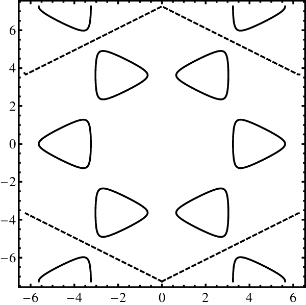
A.1.3 Metal-Insulator transition

We discuss here the metal to band insulator transition at zero temperature. In a non-interacting system, this occurs when the Fermi energy is changed such that all occupied bands become completely full, as shown in Fig. 10. In the insulator, the Fermi energy lies in between two bands and thus the filled states are separated from the empty states by a finite energy gap. As the Fermi energy is tuned, the Fermi energy might touch one of the bands thereby rendering the system metallic. Close to this transition, the energy is quadratic in the momentum $k$ , i.e., $|k|\propto|\delta\mu|^{1/2}$ . This implies that,

\displaystyle|\delta k|

\displaystyle\propto

\displaystyle|\delta\mu|^{1/2}.

(76)

Following the scaling convention in Eq. (17), we adduce a similar exponent

\displaystyle\upsilon_{L}=1/2

(77)

that governs the scaling of the modulation lengths with the shift $\delta\mu$ of the chemical potential (instead of temperature variations).

A.1.4 Dirac systems

The low energy physics of graphene and Dirac systems is characterized by the existence of Dirac points in momentum space where the density of states vanishes and the energy, $\epsilon(k)$ is proportional to the momentum $k$ for small $k$ . When we invoke and repeat our earlier analysis to these systems, we discern a trivial exponent

	$\displaystyle\|\delta k\|$	$\displaystyle\propto$	$\displaystyle\|\delta\mu\|$		(78)
		$\displaystyle\implies$	$\displaystyle\upsilon_{Dirac}=1.$		(78)

This exponent may be contrasted with that derived from Eq. (77).

A.1.5 Topological Insulators – Multiple length scale exponents as a function of the chemical potential $\mu$

The quintessential low energy physics of three-dimensional topological insulators can be gleaned from the following effective Hamiltonian[83] in momentum space,

	$\displaystyle H(\vec{k})$	$\displaystyle=$	$\displaystyle\epsilon_{0}(\vec{k})I_{4\times 4}+$
			$\displaystyle\left(\begin{array}[]{cccc}{\cal M}(\vec{k})&A_{1}k_{z}&0&A_{2}k_{-}\\ A_{1}k_{z}&-{\cal M}(\vec{k})&A_{2}k_{-}&0\\ 0&A_{2}k_{+}&{\cal M}(\vec{k})&-A_{1}k_{z}\\ A_{2}k_{+}&0&-A_{1}k_{z}&-{\cal M}(\vec{k})\end{array}\right)$

where $\epsilon_{0}(\vec{k})=C+D_{1}k_{z}^{2}+D_{2}k_{\perp}^{2}$ , ${\cal M}(\vec{k})=M-B_{1}k_{z}^{2}-B_{2}k_{\perp}^{2}$ , with $k_{\pm}=k_{x}+ik_{y}$ , $k_{\perp}=\sqrt{k_{x}^{2}+k_{y}^{2}}$ and $A_{1}$ , $A_{2}$ , $B_{1}$ , $B_{2}$ , $C$ , $D_{1}$ and $D_{2}$ constants for a given system. The energy bands are given by

\displaystyle\epsilon(\vec{k})=\epsilon_{0}(\vec{k})\pm\sqrt{{\cal M}(\vec{k})^{2}+A_{1}k_{z}^{2}+A_{2}k_{\perp}^{2}}.

(84)

These bands are plotted in Figs. 15 and 15. The finite gap between the two bands leads to an exponentially damped hopping amplitude, characterized by a finite correlation length when the Fermi energy lies within this gap. These energy bands disperse quadratically for small $k$ thus yielding

	$\displaystyle\|\delta k\|$	$\displaystyle\propto$	$\displaystyle\sqrt{\|\delta\mu\|}$		(85)
		$\displaystyle\implies$	$\displaystyle\upsilon_{bulk}=1/2$		(85)

whenever the correlation length diverges and a insulator to metal transition takes place in the bulk, thus allowing long range hopping. The same exponent is also expected whenever the modulation length becomes constant as $\mu$ crosses some threshold value.

The effective Hamiltonian for the surface states is given by

\displaystyle H_{surf}=\left(\begin{array}[]{cc}0&A_{2}k_{-}\\ A_{2}k_{+}&0\end{array}\right),

leading trivially to surface energies

\displaystyle\epsilon_{surf}(k_{x},k_{y})=\pm A_{2}k_{\perp}.

(89)

Similar to the Dirac points in graphene (see Fig. 15), we trivially find an exponent of

\displaystyle\upsilon_{surf}=1.

(90)

A.1.6 An example of a zero temperature Fermi system in which $\upsilon_{L}$ is not half or one

Very large (or divergent) effective electronic masses $m_{eff}$ can be found in heavy fermion systems (and at putative quantum critical points).[84, 85] If the electronic dispersion $\epsilon(\vec{k})$ has a minimum at $\vec{k}_{0}$ then a Taylor expansion about that minimum trivially reads

	$\displaystyle\epsilon(\vec{k})=\epsilon(\vec{k}_{0})+\frac{\hbar^{2}}{2}\sum_{ij}\left(m^{-1}_{eff}\right)_{ij}(k_{i}-k_{0i})(k_{j}-k_{0j})+$
	$\displaystyle\sum_{ijl}A_{ijl}(k_{i}-k_{0i})(k_{j}-k_{0j})(k_{l}-k_{0l})+\ldots.$		(91)

When present, parity relative to $\vec{k}_{0}$ or other considerations may limit this expansion to contain only even terms. As an example, we consider the dispersion

\displaystyle\epsilon(k)=c_{1}-c_{2}(k^{2}-k_{0}^{2})^{4},

(92)

where $c_{2}>0$ . The hopping correlation function of such a system has a term which exhibits modulations at wave-vector $k=k_{0}$ at $\mu=\mu_{*}=c_{1}$ . At higher values of the chemical potential, such a term ceases to exist. At lower values ( $\mu=\mu_{*}-\delta\mu$ ), this term breaks up into two terms whose modulation wave-vectors are different from $k_{0}$ by,

	$\displaystyle k-k_{0}$	$\displaystyle\sim$	$\displaystyle\pm\frac{\delta\mu^{1/4}}{2k_{0}c_{2}^{1/4}},$		(93)
		$\displaystyle\implies$	$\displaystyle\upsilon_{L}=1/4.$		(93)

A.2 Finite temperature length scales – Scaling as a function of temperature

At finite temperatures, apart from the modulation lengths, there generally is a set of characteristic correlation lengths. From Eq. (64), these are obtained by finding the poles (or other singularities) of the Fermi function. Along some direction $\hat{e}_{0}$ , the wave-vector $\vec{k}_{0}=\hat{e}_{0}k_{0}$ is associated with a pole $k_{0}=\pm 2\pi/L_{0}\pm i/\xi_{0}$ . At this wave-vector,

\displaystyle\epsilon(\vec{k_{0}})=\mu+\frac{2n+1}{\beta}i,

(94)

where $n$ is an integer. For a given $\mu$ , let us suppose that as we change the temperature, at $T=T_{0}$ , we reach a saddle point of $\epsilon(\vec{k})$ in the complex plane of one of the Cartesian components of $\vec{k}$ . Then, near this saddle point, the corresponding correlation and modulation lengths scale as,

	$\displaystyle\|L_{D}-L_{D0}\|$	$\displaystyle\propto$	$\displaystyle\|T-T_{0}\|^{\nu_{L}},$
	$\displaystyle\|\xi-\xi_{0}\|$	$\displaystyle\propto$	$\displaystyle\|T-T_{0}\|^{\nu_{c}},$		(95)

where $\nu_{L}=\nu_{c}=1/2$ in most cases (when the second derivative is not zero).

Appendix B Euler-Lagrange equations for scalar spin systems

We elaborate on the Euler-Lagrange equations associated with the free energy of Eq. (54) in Sec. IX. These assume the form,

	$\displaystyle\int d^{d}y\tilde{V}(\vec{x}-\vec{y})S(\vec{y})+\mu S(\vec{x})$
	$\displaystyle+u(S^{2}(\vec{x})-1)S(\vec{x})=0,$		(96)

where $\tilde{V}(\vec{x})=[V(\vec{x})+V(-\vec{x})]/2$ . For example, if we consider the finite ranged system for which,

	$\displaystyle\int d^{d}y\tilde{V}(\vec{x}-\vec{y})S(\vec{y})$	$\displaystyle=$	$\displaystyle a\nabla^{2}S(\vec{x})$		(97)
			$\displaystyle~+b\nabla^{4}S(\vec{x})+\ldots,$		(97)

then, we have,

	$\displaystyle a\nabla^{2}S(\vec{x})$	$\displaystyle+$	$\displaystyle b\nabla^{4}S(\vec{x})+\ldots+\mu S(\vec{x})$		(98)
		$\displaystyle+$	$\displaystyle u(S^{2}(\vec{x})-1)S(\vec{x})=0.$		(98)

For lattice systems, the Euler Lagrange equation (96) reads

	$\displaystyle\sum_{\vec{y}}\tilde{V}(\vec{x}-\vec{y})S(\vec{y})$	$\displaystyle+$	$\displaystyle\mu S(\vec{x})$		(99)
		$\displaystyle+$	$\displaystyle u(S^{2}(\vec{x})-1)S(\vec{x})=0.$		(99)

In general, it may be convenient to express the linear terms in the above equation in terms of the lattice Laplacian $\Delta$ . We write

\displaystyle D(\Delta)S(\vec{x})\equiv\sum_{\vec{y}}\tilde{V}(\vec{x}-\vec{y})S(\vec{y})+\mu S(\vec{x}),

(100)

$D$ being some operator which is a function of the lattice Laplacian $\Delta$ . The real-space lattice Laplacian $\Delta$ , given by the Fourier transform of Eq. (7), acts on a general field $f$ as

\Delta f(\vec{x})\equiv-\sum_{i=1}^{d}[f(\vec{x}+\hat{e}_{i})+f(\vec{x}-\hat{e}_{i})-2f(\vec{x})].

(101)

Here, $\{\hat{e}_{i}\}$ denote unit vectors along the Cartesian directions. (In the continuum limit, $\Delta$ can be replaced by $-\nabla^{2}$ .) The Euler-Lagrange equation then, takes the form,

\displaystyle D(\Delta)S(\vec{x})+u(S^{2}(\vec{x})-1)S(\vec{x})=0.

(102)

Equation 97 corresponds, on the lattice, to

	$\displaystyle\sum_{\vec{y}}\tilde{V}(\vec{x}-\vec{y})S(\vec{y})$		$\displaystyle=$		(103)
			$\displaystyle-a\Delta S(\vec{x})+b\Delta^{2}S(\vec{x})+\ldots.$		(103)

The Euler Lagrange equation for this finite ranged system reads

	$\displaystyle-a\Delta S(\vec{x})$	$\displaystyle+$	$\displaystyle b\Delta^{2}S(\vec{x})+\ldots+\mu S(\vec{x})$		(104)
		$\displaystyle+$	$\displaystyle u(S^{2}(\vec{x})-1)S(\vec{x})=0.$		(104)

References

[1] A. Mesaros, K. Fujita, H. Eisaki, S. Uchida, J. C. Davis, S. Sachdev, J. Zaanen, M. J. Lawler, and E.-A. Kim, Science 333, 426 (2011).
[2] M. B. Salamon and M. Jaime, Rev. Mod. Phys. 73, 583 (2001).
[3] B. Kalisky, J. R. Kirtley, J. G. Analytis, J.-H. Chu, A. Vailionis, I. R. Fisher, and K. A. Moler, Phys. Rev. B 81, 184513 (2010).
[4] J. R. Kirtley, B. Kalisky, L. Luan, and K. A. Moler, Phys. Rev. B 81, 184514 (2010).
[5] J. M. Tranquada, B. J. Sternlieb, J. D. Axe, Y. Nakamura, and S. Uchida, Nature 375, 561 (1995).
[6] K. Yamada, C. H. Lee, K. Kurahashi, J. Wada, S. Wakimoto, S. Ueki, H. Kimura, Y. Endoh, S. Hosoya, G. Shirane, et al., Phys. Rev. B 57, 6165 (1998).
[7] S. R. White and D. J. Scalapino, Phys. Rev. Lett. 80, 1272 (1998).
[8] J. Zaanen and O. Gunnarsson, Phys. Rev. B 40, 7391 (1989).
[9] Kazushige and Machida, Physica C: Superconductivity 158, 192 (1989).
[10] V. Emery and S. Kivelson, Physica C: Superconductivity 209, 597 (1993).
[11] A. A. Koulakov, M. M. Fogler, and B. I. Shklovskii, Phys. Rev. Lett. 76, 499 (1996).
[12] M. P. Lilly, K. B. Cooper, J. P. Eisenstein, L. N. Pfeiffer, and K. W. West, Phys. Rev. Lett. 82, 394 (1999).
[13] R. Du, D. Tsui, H. Stormer, L. Pfeiffer, K. Baldwin, and K. West, Solid State Communications 109, 389 (1999).
[14] D. G. Ravenhall, C. J. Pethick, and J. R. Wilson, Phys. Rev. Lett. 50, 2066 (1983).
[15] G. Watanabe, T. Maruyama, K. Sato, K. Yasuoka, and T. Ebisuzaki, Phys. Rev. Lett. 94, 031101 (2005).
[16] M. Seul and R. Wolfe, Phys. Rev. A 46, 7519 (1992).
[17] A. D. Stoycheva and S. J. Singer, Phys. Rev. E 65, 036706 (2002).
[18] G. Malescio and G. Pellicane, Nat Mater 2, 97 (2003).
[19] G. Malescio and G. Pellicane, Phys. Rev. E 70, 021202 (2004).
[20] M. A. Glaser, G. M. Grason, R. D. Kamien, A. KoÅ¡mrlj, C. D. Santangelo, and P. Ziherl, EPL (Europhysics Letters) 78, 46004 (2007).
[21] C. J. Olson Reichhardt, C. Reichhardt, and A. R. Bishop, Phys. Rev. Lett. 92, 016801 (2004).
[22] J. Zaanen, Nature 404, 714 (2000).
[23] S. A. Kivelson, I. P. Bindloss, E. Fradkin, V. Oganesyan, J. M. Tranquada, A. Kapitulnik, and C. Howald, Rev. Mod. Phys. 75, 1201 (2003).
[24] B. Różycki, T. R. Weikl, and R. Lipowsky, Phys. Rev. Lett. 100, 098103 (2008).
[25] S. W. Hui and N. B. He, Biochemistry 22, 1159 (1983).
[26] K. L. Babcock and R. M. Westervelt, Phys. Rev. A 40, 2022 (1989).
[27] A. Giuliani, J. L. Lebowitz, and E. H. Lieb, Phys. Rev. B 76, 184426 (2007).
[28] A. Vindigni, N. Saratz, O. Portmann, D. Pescia, and P. Politi, Phys. Rev. B 77, 092414 (2008).
[29] B. Ma, B. Yao, T. Ye, and M. Lei, Journal of Applied Physics 107, 073107 (2010).
[30] M. Seul and D. Andelman, Science 267, 476 (1995).
[31] A. Giuliani, J. L. Lebowitz, and E. H. Lieb, Phys. Rev. B 74, 064420 (2006).
[32] C. Ortix, J. Lorenzana, and C. Di Castro, Phys. Rev. B 73, 245117 (2006).
[33] I. Daruka and Z. Gulácsi, Phys. Rev. E 58, 5403 (1998).
[34] D. G. Barci and D. A. Stariolo, Phys. Rev. B 79, 075437 (2009).
[35] The order of the derivative $m$ in Eq. (12) is zero if $G(k)$ has a pole of finite order at $k=K$ , and $m\geq 0$ for the branch points.
[36] If we do not have any pole or branch point of the Fourier space correlation function, the form of the real space correlation function is governed by the endpoints of the $k$ -space integration. Therefore, in the continuum, no finite modulation length is allowed. The same is true for the correlation length.
[37] R. J. Elliott, Phys. Rev. 124, 346 (1961).
[38] M. E. Fisher and W. Selke, Phys. Rev. Lett. 44, 1502 (1980).
[39] R. B. Griffiths, Fundamental problems in statistical mechanics VII (H. van Beijeren, Amsterdam, North Holland, 1990), pp. 69–110.
[40] An initial and far more cursory treatment appeared in Z. Nussinov, arXiv:cond-mat/0506554 (2005), unpublished.
[41] Z. Nussinov, Phys. Rev. B 69, 014208 (2004).
[42] S. Chakrabarty and Z. Nussinov, Phys. Rev. B 84, 144402 (2011a).
[43] See Eq. (C29) of Ref. [41].
[44] W. Selke, Physics Reports 170, 213 (1988).
[45] Z. Nussinov, J. Rudnick, S. A. Kivelson, and L. N. Chayes, Phys. Rev. Lett. 83, 472 (1999).
[46] L. Chayes, V. Emery, S. Kivelson, Z. Nussinov, and G. Tarjus, Physica A: Statistical Mechanics and its Applications 225, 129 (1996).
[47] T. R. Kirkpatrick and D. Thirumalai, Journal of Physics A: Mathematical and General 22, L149 (1989).
[48] $G$ is a function of $k^{2}$ for rotationally symmetric systems. Similarly, for a reflection invariant system (invariant under $k_{l}\to-k_{l}$ ), $G$ is a function of $(k_{l}^{2})$ when $k_{l^{\prime}\neq l}$ are held fixed. The results described in Sec. IV.5 hold, mutatis mutandis, for any component $k_{l}$ in such reflection invariant systems.
[49] Z. Nussinov, arXiv:cond-mat/0105253 (2001) – in particular, see footnote [20] therein for the Ising ground states.
[50] S. Chakrabarty and Z. Nussinov, Phys. Rev. B 84, 064124 (2011b).
[51] An $O(n)$ system is one for which the order parameter $\vec{S}(\vec{x})$ has $n$ components normalized as $\vec{S}(\vec{x})\cdot\vec{S}(\vec{x})=n$ . The large $n$ limit of this system is equivalent to the spherical model where the spins are constrained only by the relation $\sum_{\vec{x}}(S(\vec{x}))^{2}=N$ , where $N$ is the number of lattice sites. See H. E. Stanley, Phys. Rev. 176, 2, 718 (1968).
[52] H. E. Stanley, Phys. Rev. 176, 718 (1968).
[53] T. H. Berlin and M. Kac, Phys. Rev. 86, 821 (1952).
[54] P. Bak and J. von Boehm, Phys. Rev. B 21, 5297 (1980).
[55] A. Gendiar and T. Nishino, Phys. Rev. B 71, 024404 (2005).
[56] S. Redner and H. E. Stanley, J. Phys. C 10, 4765 (1977a).
[57] S. Redner and H. E. Stanley, Phys. Rev. B 16, 4901 (1977b).
[58] J. Oitmaa, J. Phys. A 18, 365 (1985).
[59] D. Mukamel, J. Phys. A 10, L249 (1977).
[60] R. M. Hornreich, M. Luban, and S. Shtrikman, Phys. Rev. Lett. 35, 1678 (1975).
[61] K. Zhang and P. Charbonneau, Phys. Rev. B 83, 214303 (2011).
[62] P. Bak, Reports on Progress in Physics 45, 587 (1982).
[63] We thank Michael Ogilvie for prompting us to think about this generalization.
[64] C. M. Bender and S. Boettcher, Phys. Rev. Lett. 80, 5243 (1998).
[65] B. Josephson, Physics Letters 21, 608 (1966), ISSN 0031-9163.
[66] M. Peskin and D. Schroeder, An introduction to quantum field theory, Advanced book program (Westview Press, 2007).
[67] C. A. Regal, M. Greiner, and D. S. Jin, Phys. Rev. Lett. 92, 040403 (2004).
[68] M. W. Zwierlein, C. A. Stan, C. H. Schunck, S. M. F. Raupach, A. J. Kerman, and W. Ketterle, Phys. Rev. Lett. 92, 120403 (2004).
[69] T.-L. Ho and R. B. Diener, Phys. Rev. Lett. 94, 090402 (2005).
[70] Z. Nussinov and S. Nussinov, Phys. Rev. A 74, 053622 (2006).
[71] H. Thomas, Nonlinear dynamics in solids (Springer-Verlag, 1992).
[72] J. Schmalian and P. G. Wolynes, Phys. Rev. Lett. 85, 836 (2000).
[73] D. Hu, P. Ronhovde, and Z. Nussinov, Philosophical Magazine 92, 406 (2012).
[74] J. C. Sprott, American Journal of Physics 68, 758 (2000).
[75] Y. Pomeau and P. Manneville, Communications in Mathematical Physics 74, 189 (1980).
[76] T. Park, Z. Nussinov, K. R. A. Hazzard, V. A. Sidorov, A. V. Balatsky, J. L. Sarrao, S.-W. Cheong, M. F. Hundley, J.-S. Lee, Q. X. Jia, et al., Phys. Rev. Lett. 94, 017002 (2005).
[77] S. Pankov and V. Dobrosavljević, Phys. Rev. Lett. 94, 046402 (2005).
[78] Z. Nussinov, I. Vekhter, and A. V. Balatsky, Phys. Rev. B 79, 165122 (2009).
[79] J. W. Clark, M. V. Zverev, and V. A. Khodel, arXiv:cond-mat.str-el/1203.3201 (2012).
[80] D. Ma, A. D. Stoica, and X.-L. Wang, Nat Mater 8, 30 (2009).
[81] G. Grüner, Rev. Mod. Phys. 60, 1129 (1988).
[82] G. Grüner, Density Waves In Solids, Frontiers in Physics (Perseus Pub., 2000).
[83] H. Zhang, C.-X. Liu, X.-L. Qi, X. Dai, Z. Fang, and S.-C. Zhang, Nat. Phys. 5, 438 (2009).
[84] C. M. Varma, Z. Nussinov, and W. van Saarloos, Physics Reports 361, 267 (2002).
[85] P. Coleman, C. Pépin, Q. Si, and R. Ramazashvili, Journal of Physics: Condensed Matter 13, R723 (2001).

	$\displaystyle\|L_{D}-L_{D0}\|$	$\displaystyle\propto$	$\displaystyle\|T-T_{0}\|^{\nu_{L}},$
	$\displaystyle\|\xi-\xi_{0}\|$	$\displaystyle\propto$	$\displaystyle\|T-T_{0}\|^{\nu_{c}},$		(95)