Multilevel Sparse Kernel-Based Interpolation
Abstract
A multilevel kernel-based interpolation method, suitable for moderately high-dimensional function interpolation problems, is proposed. The method, termed multilevel sparse kernel-based interpolation (MLSKI, for short), uses both level-wise and direction-wise multilevel decomposition of structured (or mildly unstructured) interpolation data sites in conjunction with the application of kernel-based interpolants with different scaling in each direction. The multilevel interpolation algorithm is based on a hierarchical decomposition of the data sites, whereby at each level the detail is added to the interpolant by interpolating the resulting residual of the previous level. On each level, anisotropic radial basis functions are used for solving a number of small interpolation problems, which are subsequently linearly combined to produce the interpolant. MLSKI can be viewed as an extension of -boolean interpolation (which is closely related to ideas in sparse grid and hyperbolic crosses literature) to kernel-based functions, within the hierarchical multilevel framework to achieve accelerated convergence. Numerical experiments suggest that the new algorithm is numerically stable and efficient for the reconstruction of large data in , for , with tens or even hundreds of thousands data points. Also, MLSKI appears to be generally superior over classical radial basis function methods in terms of complexity, run time and convergence at least for large data sets.
keywords
kernel-based interpolation, radial basis functions, multilevel, -boolean interpolation, sparse grids, hyperbolic crosses.AMS
65F10, 65N30, 65N221 Introduction
Over the last four decades, radial basis functions (RBFs) have been successfully applied to (scattered) data interpolation/approximation in (see, e.g., [49] and the references therein for a literature review). The interest on kernel-based and, in particular, on RBF interpolants can be traced in their ability to produce global interpolants of user-defined smoothness without the shortcomings of multivariate polynomial interpolation. These interpolants admit generally good convergence properties and they can be implemented in (essentially) dimension-independent fashion, making them potentially attractive for a number of applications.
Despite the above attractive properties, RBF interpolation can be cumbersome in practice. Solving the resulting linear system is challenging due to both the density and the ill-conditioning of the resulting interpolation matrix (see, e.g., [12, 42]). A number of techniques have been proposed to deal with the ill-conditioning of the interpolation system.
For smooth basis functions such as the Gaussian and the multiquadric, the ill-conditioning depends crucially on a width parameter. Novel QR-based algorithms which eliminate the ill-conditioning problem for thousands of points have been developed [20, 18, 13]. An alternative family of methods, where small local problems are solved which generate approximate cardinal functions has also been proposed [16, 3]. The matrix associated with such an approach is much better conditioned, and allows for rapid solution using iterative methods. Finally, in [40], a stable interpolation algorithm on carefully selected nodes for Gaussian basis functions is given.
The introduction of RBFs with compact support [50, 47] aims to address the density issue of the interpolation matrix. Moreover, a number of techniques have been developed to reduce the complexity of calculating the interpolant, involving multipole type expansion for a variety of RBFs [3]. Using such methods is possible to compute an RBF interpolant with -computations for quasi–uniform data, where is the number of data sites though, to the best of our knowledge, we are not aware of any methods which guarantee a bounded number of iterations independently of .
Thus, the complexity of kernel-based interpolation remains a challenge when , as the number of data points is required to grow exponentially with respect to the dimension to ensure good convergence rates. It is not surprising, therefore, that the use of RBFs in practice has been largely limited to tens of thousands of data sites, which, in turn, has restricted their application to low , typically or .
This work is concerned with the introduction of a kernel-based interpolation method on structured or mildly unstructured data sites, which aims to address the computational complexity issues of RBF interpolation for , while simultaneously reducing the ill-conditioning of the resulting interpolation problem. The new scheme, termed multilevel sparse kernel-based interpolation (MLSKI), is based on a hierarchical decomposition of the data sites, whereby at each level the detail is added to the interpolant by interpolating the resulting residual of the previous level. On each level, anisotropic radial basis functions are used for solving a number of small interpolation problems, which are subsequently linearly combined to produce the interpolant; the new method can be viewed as an extension of (and, indeed, it has been inspired from) the idea of -boolean interpolation [10, 44, 36, 30, 23] to kernel-based functions, which, in turn, is closely related to ideas in sparse grid [51, 27, 4, 31, 25, 26] and hyperbolic crosses [45, 1] literature. We note that in [43] hyperbolic cross products of one dimensional RBFs have been considered. The hierarchical multilevel framework used to achieve accelerated convergence is relatively standard in the RBF literature [17, 33, 34, 28].
In the simplest setting, the MLSKI algorithm assumes that the data sites are on a Cartesian uniform grid of size in , with , for a final level . For each level of the MLSKI algorithm, we construct a sparse kernel-based interpolant of the interpolation residual as follows. We consider carefully chosen subsets of the data points of level , each subset having size data points. On each of these subsets, which we shall refer to as partial grids, we solve the interpolation problem. As the partial grids are anisotropic in nature, we employ appropriate anisotropically scaled kernels (anisotropic RBFs [8, 9, 2]) for each interpolation problem on each partial grid. Once all the interpolants on the partial grids have been computed they are linearly combined to give the total interpolant (of the residual) for level . Hence, the complexity of the resulting MLSKI algorithm is dominated by the complexity of the last step, i.e., one needs to solve interpolation problems of size and linearly combine the resulting interpolants on the partial grids. This, in turn, implies that the MLSKI algorithm admits (at least theoretically) -complexity, where is the number of grid points in each direction, and is the complexity of the univariate -point algorithm.
The computation of each interpolant on the partial grids is completely independent from the other interpolants on each level . Therefore, the MLSKI algorithm is ideally suited for implementation on parallel computers. The MLSKI algorithm is tested in practice for a number of relevant test cases with . The numerical experiments suggest that MLSKI is numerically stable in practice and efficient for the reconstruction of large data in , for , with hundreds of thousands of data points. Also, MLSKI appears to be generally superior over classical radial basis function methods in terms of complexity, run time and convergence, at least for large data sets.
The remaining of this paper is organized as follows. In Section 2, we discuss anisotropic versions of radial basis functions, suitable for interpolation on data sites with anisotropic characteristics. In Section 3, we introduce the sparse kernel-based interpolation method, which will be used in Section 4 at each level of the multilevel algorithm. The stability and implementation of the MLSKI algorithm is discussed in Section 5. A series of numerical experiments is given in Section 6, for = 2, 3, 4. In Section 7, we draw some conclusions on the new developments presented in this work and discuss possible extensions.
2 Anisotropic RBF interpolation
Radial basis functions are radially symmetric by construction having hyper-spheres as their level surfaces. However, interpolation of data with anisotropic distribution of data sites in the domain requires special consideration. To this end, anisotropic radial basis functions (ARBFs) have been introduced and used in practice [8, 9, 2]; they are also known as elliptic basis functions as they have hyper-ellipsoidal level surfaces.
Definition 1.
Let be a given RBF centred at and let be an invertible matrix. The anisotropic radial basis function is defined by .
Evidently, when is the -identity matrix. In Figure 1, the Gaussian RBF and the corresponding anisotropic Gaussian RBF centred at for are drawn. (Here, we use the notation for a diagonal matrix with diagonal entries are given by the components of the vector .)

We now discuss the the solution of an anisotropic interpolation problem. We restrict the discussion to positive definite kernels, which will be used later, though anisotropic versions of conditionally positive definite REBs is completely completely analogous.
For data sites contained in a computational domain , we consider the interpolation data . Let be a positive definite radial function and be a chosen invertible matrix. Then, the anisotropic RBF interpolant is defined by:
| (1) |
for such that the interpolation conditions , , are satisfied.
The well-posedness of the interpolation problem is guaranteed (for positive definite kernels) as a direct consequence of the invertibility of the scaling matrix . We refer to [2] for the error analysis of anisotropic RBF interpolation.
3 Sparse kernel-based interpolation
We describe the basic sparse kernel-based interpolation (SKI) method that will be used in each step of the multilevel algorithm. The SKI method can be used also as a single step interpolation method.
The starting point is the observation that, assuming sufficient smoothness of the interpolation data, the number of points required to provide a given accuracy can be dramatically reduced when basis functions with carefully constructed direction-wise anisotropic scaling are used. This way, notwithstanding the approximation strength coming from a few directions only, there is only negligible loss of accuracy, due to the additional smoothness assumed. Hyperbolic cross products and sparse grids use this idea in the context of high dimensional numerical quadrature, approximation and in numerical solution of partial differential equations.
In [43], hyperbolic crosses of tensor products of one-dimensional RBFs have been considered without numerical assessment of the resulting method. The use of non-tensor product -dimensional RBFs in the hyperbolic-cross/sparse-grid setting is not straightforward, as such approximation spaces are characterised by basis functions with differently anistropic scalings in different directions. Using such scalings would not guarantee the well-posedness of the resulting kernel-based interpolation problem.
An alternative approach can be motivated by the, so-called, -boolean interpolation [10] or, the related combination technique [27, 22], for piecewise polynomial interpolation on sparse grids. A key point in this approach is that the piecewise polynomial interpolant is equivalent to a linear combination of interpolants constructed on a carefully selected collection of subsets of the (anisotropic) basis functions. Each such subset consists of translations of the same (anisotropic) basis function.
To construct the sparse kernel-based interpolant, we solve a number of anisotropic radial basis function interpolation problems on appropriately selected sub-grids and we linearly combine the resulting partial interpolants to obtain the sparse kernel-based interpolant.
More specifically, let , and let . The extension to general axiparallel domains is straightforward; we refrain from doing so here in the interest of simplicity of the presentation only. Comments on possible extensions to more general domains will be given in Section 7.
For a multi-index , we define the family of directionally uniform grids , in , with meshsize . That is, consists of the points , with , for , . The number of nodes in is given by
If = for all is the uniform full grid of level , having size =; this will be denoted by .
We also consider the following subset of ,
| (2) |
with , which will be referred to as the sparse grid of level in dimensions. We refer to Figure 2 for a visual representation of (2) for and . Notice that there is some redundancy in this definition as some grid points are included in more than one sub-grid.
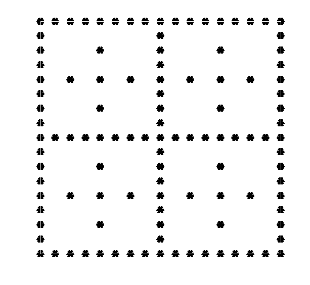
|
= |

|

|

|

|
We want to evaluate the interpolant at the constituent sub-grids . As the constituent grids admit different density in each coordinate direction, we shall make use the anisotropic RBFs from Section 2. To this end, for each multi-index , we define the transformation matrix by
The anisotropic RBF interpolant of at the points of is then defined by
| (3) |
for , where are chosen so that the interpolation conditions
are satisfied.
To construct the sparse kernel-based interpolant (SKI, for short) on the sparse grid , the sub-grid interpolants are linearly combined using the formula
| (4) |
The combination formula (4) has been used in the context of -boolean Lagrange polynomial interpolation [10], and in the combination technique for the numerical solution of elliptic partial differential equations using the finite element method on sparse grids [27, 22]. For , (4) becomes
| (5) |
that is, the first term on the right-hand side of (5) gives the sum of interpolants on the sub-grids of level , while the second term on the right-hand side of (5) subtracts the redundant points visited more than once. We refer to Figure 3 for an illustration when and .
|
|
= |
|
|
|
| |||

|

|

|
Hence, SKI uses a dimension-wise multilevel decomposition of interpolation data sites in conjunction with the application of kernel-based interpolants with different scaling in each direction. The sparse kernel-based interpolant can be implemented in a quite straightforward fashion by utilising existing, fast, RBF interpolation algorithms: the only modification needed is the introduction of a scaling for each sub-grid problem. We note that each interpolation problem can be solved completely independently, rendering the resulting SKI method ideally suited for implementation in parallel computers.
Moreover, we observe the size of each sub-grid problem is , where is the number of levels, i.e., it is independent of the dimension . One has to solve such sub-grid problems to obtain the sparse kernel-based interpolant. Observe that is the number of points of the corresponding full grid in each space direction. Hence, if the rate of convergence for the SKI algorithm is comparable with the one of the standard RBF algorithm for a sufficiently large class of underlying functions , the benefits in complexity are potentially significant, especially for . Indeed, when the underlying function is assumed to admit sufficient regularity (e.g., if the regularity of is characterised by anisotropic Sobolev spaces) [10, 27, 22] and [43] the rate of convergence on sparse grids for tensor-product of piece-wise polynomials and of one-dimensional RBFs, respectively, is shown to be optimal (modulo a logarithmic factor). Although, there is no general proof at this point that this is also the case for the SKI method presented here, numerical experiments presented below show that for the multilevel version of the SKI algorithm, described in the next section, good convergence results are also observed. We finally remark that for the case of Gaussian interpolation, due its tensor-product nature, the theoretical results of [43] on tensor-product one-dimensional sparse RBF interpolation should be applicable to the case of SKI also.
4 Multilevel Sparse Kernel-Based Interpolation
Multilevel methods for RBFs [17, 33, 48, 14, 11, 38, 28, 34, 39] combine the advantages of stationary and non-stationary interpolation, aiming to accelerate convergence and to improve the numerical stability of the interpolation procedure. The basic idea of multilevel methods in this context is to interpolate the data at the coarsest level, and then update by interpolating the residuals on progressively finer data sets using appropriately scaled basis functions.
The setting of SKI is naturally suited to be used within a multilevel interpolation algorithm. Indeed, the sparse grids from lower to higher level are nested, i.e., for ; we refer to Figure 4 for an illustration when . Moreover, each sub-grid interpolant uses appropriately scaled anisotropic basis function with the scaling being proportional to density of the corresponding constituent sub-grid. Finally, due to the geometrical progression in the problem size from one sparse grid to the next, a multilevel algorithm would not affect adversely the attractive complexity properties of SKI.
The multilevel SKI (MLSKI, for short) algorithm is initialised by computing the SKI at the coarsest designated sparse grid and set . Then, for , we compute to be the sparse grid interpolant of the residual on . The resulting multilevel sparse kernel based interpolant is then given by

5 Stability of SKI and MLSKI
The numerical stability of RBF interpolation is a challenging issue, due to the ill-conditioning of the respective interpolation matrices in standard bases; we refer to [49, 12] and the references therein for a discussion. It is, therefore, evident that the numerical stability of SKI and MLSKI algorithms can be assessed by considering the maximum condition number of the constituent sub-grid interpolation problems.
The main factors affecting the conditioning of an RBF interpolation problem are the problem size, the separation distance of the respective data set , given by
and the shape parameters of the RBF (which adjusts the “strength” or the support, depending on the type of RBF). The choice of shape parameter and the monitoring of the separation distance require more attention in practice than the problem size, which is of secondary importance [49, 12]. Recipes for choosing RBF shape parameters in various contexts have been presented, e.g., in [29, 21, 5, 6, 35, 7], while the dependence of the stability on the shape has been addressed in [41, 20, 19, 15, 13, 18], where stable algorithms for RBF interpolation with small shape parameters have been proposed.
SKI and MLSKI naturally include scaling adjustment at each level. So, the condition number of each sub-grid interpolation matrix appears to be (mildly) affected by the sub-grid size, as we shall see in Section 6. This is, indeed, a very attractive feature of the SKI and MLSKI algorithms as the growth of degrees of freedom on each sub-grid grows independently of the problem dimension .
Observing that, due to the anisotropy of the scaling matrices , the separation distance on each pulled-back (multiplied by ) sub-grid is constant with respect to the level . This suggests that we can use standard heuristics for the choice of shape-parameters for multilevel RBF interpolation (see [17, 33, 48, 14, 11, 38, 28, 34, 39], or [49] for a review). In particular, we set
| (6) |
for some constant . Extensive numerical experiments presented in [46] suggest that the choice , gives very small condition numbers at the cost of (mildly) lower accuracy of the interpolation problem. The choice , produces larger but mostly safe condition numbers (in this work we shall refer to a condition number as being safe when ), with the resulting computations admitting good convergence properties. For , we have . For , the ill-conditioning gradually increases with , resulting in unstable computations.
6 Numerical Experiments
We present a collection of numerical experiments for , where the implementation of SKI and MLSKI algorithms is assessed and compared against both the standard RBF interpolation on uniform full grids and its standard multilevel version (MLRBF); see, e.g, [49] for a review.
The algorithm implementation has been performed in MATLAB© on a quad-core 2.67GHz Intel Xeon X5550 CPU with 12GB of RAM, without taking advantage of the possibility of parallel implementation of SKI or MLSKI. The SKI/MLSKI algorithm is able to solve -variate interpolation problems on sparse grids up to centers for , and up to centers for , respectively. The same basic interpolation solver for classical RBF on the same machine could only solve problems of size nearly regardless of the dimension , due to the size of the resulting linear system.
We stress that no attempt has been made to use fast algorithms, e.g., the fast Gauss transform of Greengard and Strain [24] for the RBF interpolation problems for either the standard RBF, MLRBF or the SKI, MLSKI algorithms. The use of fast or stable algorithms for RBF interpolation could be also used within the sub-grid interpolation problems of SKI/MLSKI. Indeed, any modern fast evaluation or numerical stabilization technique in RBF interpolation of a single problem can be incorporated into the SKI/MLSKI framework, possibly substantially improving the results presented here.
6.1 Experiment 1
| SGnode | Max-error | RMS-error | Cond. no | Time |
|---|---|---|---|---|
| 9 | 6.2215e-1 | 1.8363e-1 | 2.6912e+3 | 1 |
| 21 | 3.3237e-1 | 7.6547e-2 | 2.5325e+4 | 1 |
| 49 | 1.1130e-1 | 3.8660e-2 | 2.8184e+5 | 1 |
| 113 | 4.0379e-2 | 1.0835e-2 | 2.6522e+6 | 1 |
| 257 | 1.2649e-2 | 2.5117e-3 | 2.9516e+7 | 1 |
| 577 | 2.4678e-3 | 4.0273e-4 | 1.7591e+8 | 1 |
| 1281 | 2.2043e-4 | 2.1030e-5 | 1.0484e+9 | 1 |
| 2817 | 3.5287e-5 | 2.5391e-6 | 2.3229e+9 | 5 |
| 6145 | 6.2139e-6 | 3.2696e-7 | 5.1468e+9 | 33 |
| 13313 | 1.1784e-6 | 4.2920e-8 | 6.5016e+9 | 281 |
| 28673 | 2.1204e-7 | 5.6557e-9 | 8.2129e+9 | 2397 |
| 61441 | 4.1321e-8 | 7.6854e-10 | 8.7056e+9 | 21586 |
The MLSKI algorithm with Gaussian basis functions is applied to the (standard) benchmark Franke’s function for , given by
| (7) | ||||
In Table 1, “SGnode” stands for the number of sparse grid centers used, “Max-error” and “RMS-error’ are the maximum norm and root-mean-square (-norm) errors, respectively, evaluated at Halton points [37], “Cond. no” stands for the largest -norm condition number of the sub-grid interpolation matrices. Finally, “Time” is the time in seconds required to solve the interpolation problem in the above computer. We note that the tic; and toc; commands of MATLAB© have been used to produce the run times, which is accurate for longer run times.
In Table 2, the MLSKI algorithm with Gaussian basis functions is applied to a three-dimensional version of Franke’s function , given by
| (8) | ||||
| SGnode | Max-error | RMS-error | Cond. no | Time |
|---|---|---|---|---|
| 27 | 6.8808e-1 | 1.0179e-1 | 1.4863e+4 | 1 |
| 81 | 5.5853e-1 | 7.7339e-2 | 2.5376e+5 | 1 |
| 225 | 2.4324e-1 | 3.8389e-2 | 6.2956e+4 | 1 |
| 593 | 1.5884e-1 | 2.1676e-2 | 1.0617e+7 | 8 |
| 1505 | 6.2918e-2 | 6.7591e-3 | 6.9125e+5 | 9 |
| 3713 | 1.3403e-2 | 1.7755e-3 | 4.2986e+8 | 12 |
| 8961 | 2.2041e-3 | 2.2448e-4 | 6.2618e+6 | 42 |
| 21249 | 3.3081e-4 | 2.9755e-5 | 9.2544e+9 | 328 |
| 49665 | 8.9456e-5 | 4.5151e-6 | 2.1038e+7 | 2900 |
| 114689 | 1.5829e-5 | 5.7471e-7 | 1.0594e+11 | 25160 |
Next, we consider the interpolation problem of the simple function , with
We employ the SKI algorithm for ; the results are given in Table 3.
| SGnode | Max-error | RMS-error | Cond. no | Time |
|---|---|---|---|---|
| 81 | 7.9105e-2 | 4.4589e-2 | 3.6544e+5 | 1 |
| 297 | 2.4067e-2 | 1.0677e-2 | 8.6224e+6 | 1 |
| 945 | 1.9844e-2 | 6.3598e-3 | 1.0568e+6 | 1 |
| 2769 | 5.6653e-3 | 1.2672e-3 | 3.6076e+8 | 2 |
| 7681 | 4.7096e-3 | 8.2613e-4 | 1.4065e+7 | 14 |
| 20481 | 1.3155e-3 | 1.5425e-4 | 1.4848e+10 | 164 |
| 52993 | 1.1548e-3 | 1.0690e-4 | 1.2741e+8 | 1766 |
| 133889 | 3.2099e-4 | 1.9243e-5 | 6.0115e+11 | 16442 |
| 331777 | 2.8385e-4 | 1.3934e-5 | 1.1542e+9 | 169643 |
6.2 Experiment 2
We now turn our attention to the conditioning of the sub-grid interpolation problems. In the previous experiment a, mostly safe, maximum condition number for each level’s sub-grid interpolation problems is observed, using in (6). Here, we investigate the choice which gives condition numbers at the cost of a slight reduction in the quality of the approximation in the MLSKI algorithm.
The results from the MLSKI algorithm using Gaussians with shape parameter chosen from (6) with are given in Table 4. The “Time”-column is ommitted for brevity as it is almost identical to the one of Table 2. We observe that the error is roughly 5 times worse, but the condition numbers of the resulting sub-grid problems are nearly optimal.
| SGnode | Max-error | RMS-error | Cond. no |
|---|---|---|---|
| 27 | 7.0968e-1 | 1.0531e-1 | 1.8 |
| 81 | 5.5864e-1 | 7.6444e-2 | 2.6 |
| 225 | 3.2513e-1 | 4.8817e-2 | 1.5 |
| 593 | 1.3272e-1 | 1.5118e-2 | 3.0 |
| 1505 | 7.8689e-2 | 7.9827e-3 | 1.5 |
| 3713 | 2.1970e-2 | 2.1392e-3 | 3.2 |
| 8961 | 1.0543e-2 | 9.9965e-4 | 1.6 |
| 21249 | 1.7569e-3 | 1.7839e-4 | 3.4 |
6.3 Experiment 3
We continue by comparing the SKI and MLSKI algorithms with standard RBF interpolation on full grids and with its (standard) multilevel version on full grids, henceforth denoted by MLRBF.
In Figure 5, the root mean-square error of RBF, MLRBF, SKI and MLSKI, respectively, for , are plotted against the number of data sites and against the computation time (in seconds). For RBF and MLRBF, denotes the number of data sites on the full grid , whereas for SKI and MLSKI, refers to the number of sparse grid nodes (i.e., SGnode). (We note in passing that using standard “isotropic” RBF interpolation on sparse grids does not appear to result to a convergent algorithm.) The choice of the shape parameter is given by (6) with for SKI/MLSKI for all experiments; the shape parameter for RBF/MLRBF is chosen so as to have comparable condition numbers in all cases. We observe that RBF/MLRBF interpolation appears to perform better than SKI/MLSKI when the error is plotted against . The SKI/MLSKI algorithms are, on the other hand, able to calculate larger problems and they do so efficiently in terms of complexity, at least for the case of larger problems. This is manifested in the RMS-error versus computation time plot in Figure 5.
As discussed in Section 3, -Boolean Lagrange interpolation using polynomials requires additional smoothness of mixed derivatives in order to ensure the essentially optimal convergence rate. To test the extend to which this is also the case for the MLSKI algorithm, we consider the function , with
This function does not posses smooth mixed derivatives of (arbitrarily) high order. In Figure 6, the root mean-square error of RBF, MLRBF, SKI and MLSKI, respectively, for , are plotted against the number of data sites and against the computation time (in seconds). Somewhat surprisingly, we observe that the MLSKI algorithm outperforms RBF/MLRBF interpolation both in terms of degrees of freedom and in terms of computational time, at least for larger problems.
Next, we turn our attention to the problem of interpolating five-dimensional data, i.e., . This is a challenge in practice with known methods: standard RBF interpolation is limited to few tens of thousands of data points. This, in turn, results to using data points in each coordinate direction, thereby, limiting the resulting approximation quality.
We compare the four interpolation methods on a four-variate version of the Franke’s function , with
as well as the four-variate version of , which is defined completely analogously. The convergence history, given in Figures 7 and 8, respectively, indicates similar behaviour to the three-dimensional case. The choice in the shape parameter is as in (6) with . We remark on the favourable complexity of the MLSKI algorithm compared to RBF/MLRBF as grows. Indeed, the MLSKI algorithm is able to compute highly accurate interpolants, as large can be achieved using moderate computational time.
6.4 Experiment 4
It is easy to see that -dimensional Gaussian kernels are tensor-products of one-dimensional ones. Hence, it is interesting to also consider SKI and MLSKI with non-Gaussian kernels.
To this end, we consider the problem of interpolation of using Wendland’s compactly the supported kernel . In Figure 9 the convergence history of the various interpolation methods based on the compactly supported kernel are given. The choice in the shape parameter is as in (6) with , resulting in safe conditions numbers for all methods. Interestingly, the SKI method seems to converge very slowly, while the MLSKI algorithm appears to perform well.
Finally, we consider the problem of interpolation of and using the inverse multiquadric kernel with the above choice of the shape parameter. The results are given in Figures 10 and 11, respectively. Again, for the case of the SKI methods seems to be performing poorly, compared to the fast convergence of MLSKI.
7 Concluding remarks
A multilevel kernel-based interpolation method, suitable for moderately high-dimensional interpolation problems on carefully structured grids has been proposed. The key idea is the use of hierarchical decomposition of the data sites with anisotropic radial basis functions used on each level, solving a number of smaller independent interpolation problems. MLSKI appears to be generally superior over classical radial basis function methods in terms of complexity, run time and convergence, at least for large data sets when . It is expected that good convergence can be obtained for also.
Currently, the choice of data sets (sparse grids) is highly structured. Some preliminary numerical experiments for SKI on mildly perturbed sparse grids, presented in [46], indicate that the SKI method converges with the same rate, albeit with a somewhat larger constant. Perhaps a more robust methodology for extending the applicability of SKI/MLSKI methods to scattered data is the pre-computation of the values on the corresponding sparse grid data sites via local interpolation. The extension of the SKI/MLSKI method to more general geometries could possibly be handled either by introducing fictitious gridded data sites with suitable data values, taking into account the nature of the data, or by conformally mapping the computational domain [32].
The discussion in this work has been confined to strictly positive definite kernels. The implementation of MLSKI with conditionally positive definite kernels is subject to ongoing work; some preliminary results can be found in [46].
References
- [1] K. I. Babenko, Approximation by trigonometric polynomials in a certain class of periodic functions of several variables, Soviet Math. Dokl., 1 (1960), pp. 672–675.
- [2] R. Beatson, O. Davydov, and J. Levesley, Error bounds for anisotropic RBF interpolation, J. Approx. Theory, 162 (2010), pp. 512–527.
- [3] R. K. Beatson, J. B. Cherrie, and C. T. Mouat, Fast fitting of radial basis functions: methods based on preconditioned GMRES iteration, Adv. Comput. Math., 11 (1999), pp. 253–270. Radial basis functions and their applications.
- [4] H.-J. Bungartz, M. Griebel, and U. Rüde, Extrapolation, combination, and sparse grid techniques for elliptic boundary value problems, Comput. Methods Appl. Mech. Engrg., 116 (1994), pp. 243–252. ICOSAHOM’92 (Montpellier, 1992).
- [5] R. E. Carlson and T. A. Foley, The parameter in multiquadric interpolation, Comput. Math. Appl., 21 (1991), pp. 29–42.
- [6] , Interpolation of track data with radial basis methods, Comput. Math. Appl., 24 (1992), pp. 27–34. Advances in the theory and applications of radial basis functions.
- [7] R. E. Carlson and B. K. Natarajan, Sparse approximate multiquadric interpolation, Comput. Math. Appl., 27 (1994), pp. 99–108.
- [8] G. Casciola, D. Lazzaro, L. B. Montefusco, and S. Morigi, Shape preserving surface reconstruction using locally anisotropic radial basis function interpolants, Comput. Math. Appl., 51 (2006), pp. 1185–1198.
- [9] G. Casciola, L. B. Montefusco, and S. Morigi, The regularizing properties of anisotropic radial basis functions, Appl. Math. Comput., 190 (2007), pp. 1050–1062.
- [10] F.-J. Delvos, -variate Boolean interpolation, J. Approx. Theory, 34 (1982), pp. 99–114.
- [11] G. E. Fasshauer, Solving differential equations with radial basis functions: multilevel methods and smoothing, Adv. Comput. Math., 11 (1999), pp. 139–159. Radial basis functions and their applications.
- [12] , Meshfree approximation methods with MATLAB, vol. 6 of Interdisciplinary Mathematical Sciences, World Scientific Publishing Co. Pte. Ltd., Hackensack, NJ, 2007. With 1 CD-ROM (Windows, Macintosh and UNIX).
- [13] G. E. Fasshauer and Mccourt M. J., Stable evaluation of Gaussian RBF interpolants, Submitted for publication, (2011).
- [14] G. E. Fasshauer and J. W. Jerome, Multistep approximation algorithms: improved convergence rates through postconditioning with smoothing kernels, Adv. Comput. Math., 10 (1999), pp. 1–27.
- [15] G. E. Fasshauer and J. G. Zhang, On choosing “optimal” shape parameters for RBF approximation, Numer. Algorithms, 45 (2007), pp. 345–368.
- [16] A. C. Faul and M. J. D. Powell, Proof of convergence of an iterative technique for thin plate spline interpolation in two dimensions, Adv. Comput. Math., 11 (1999), pp. 183–192.
- [17] M. S. Floater and A. Iske, Multistep scattered data interpolation using compactly supported radial basis functions, J. Comput. Appl. Math., 73 (1996), pp. 65–78.
- [18] B. Fornberg, E. Larsson, and N. Flyer, Stable computation with Gaussian radial basis functions, SIAM J. Sci. Comput., 33 (2011), pp. 869–892.
- [19] B. Fornberg and C. Piret, A stable algorithm for flat radial basis functions on a sphere, SIAM J. Sci. Comput., 30 (2007/08), pp. 60–80.
- [20] B. Fornberg and G. Wright, Stable computation of multiquadric interpolants for all values of the shape parameter, Comput. Math. Appl., 48 (2004), pp. 853–867.
- [21] R. Franke, Scattered data interpolation: tests of some methods, Math. Comp., 38 (1982), pp. 181–200.
- [22] J. Garcke and M. Griebel, On the parallelization of the sparse grid approach for data mining, in Large-Scale Scientific Computations, Third International Conference, LSSC 2001, Sozopol, Bulgaria, S. Margenov, J. Wasniewski, and P. Yalamov, eds., vol. 2179 of Lecture Notes in Computer Science, Springer, 2001, pp. 22–32. also as SFB 256 Preprint 721, Universität Bonn, 2001.
- [23] J. Garcke and M. Hegland, Fitting multidimensional data using gradient penalties and the sparse grid combination technique, Computing, 84 (2009), pp. 1–25.
- [24] L. Greengard and J. Strain, The fast Gauss transform, SIAM J. Sci. Statist. Comput., 12 (1991), pp. 79–94.
- [25] M. Griebel, Adaptive sparse grid multilevel methods for elliptic PDEs based on finite differences, Computing, 61 (1998), pp. 151–179.
- [26] M. Griebel and F. Koster, Multiscale methods for simulation of turbulent flow, in Herschel, E, editers, Numerical Flow Simulation, vol. 82 of Notes on Numerical Fluid Mechanics and Multidisciplinary design, Springer-Verlag, 2003, pp. 203–214.
- [27] M. Griebel, M. Schneider, and C. Zenger, A combination technique for the solution of sparse grid problems, in Iterative methods in linear algebra (Brussels, 1991), North-Holland, Amsterdam, 1992, pp. 263–281.
- [28] S. J. Hales and J. Levesley, Error estimates for multilevel approximation using polyharmonic splines, Numer. Algorithms, 30 (2002), pp. 1–10.
- [29] R. L. Hardy, Multiquadrics of topography and other irregular surface, J. Geophys Res, 76 (1971), pp. 1905–1915.
- [30] M. Hegland, J. Garcke, and V. Challis, The combination technique and some generalisations, Linear Algebra and its Applications, 420 (2007), pp. 249–275.
- [31] P. W. Hemker, Sparse-grid finite-volume multigrid for D-problems, Adv. Comput. Math., 4 (1995), pp. 83–110.
- [32] A. R. H. Heryudono and T. A. Driscoll, Radial basis function interpolation on irregular domain through conformal transplantation, J. Sci. Comput., 44 (2010), pp. 286–300.
- [33] A. Iske, Hierarchical scattered data filtering for multilevel interpolation schemes, in Mathematical methods for curves and surfaces (Oslo, 2000), Innov. Appl. Math., Vanderbilt Univ. Press, Nashville, TN, 2001, pp. 211–221.
- [34] A. Iske and J. Levesley, Multilevel scattered data approximation by adaptive domain decomposition, Numer. Algorithms, 39 (2005), pp. 187–198.
- [35] E. J. Kansa and R. E. Carlson, Improved accuracy of multiquadric interpolation using variable shape parameters, Comput. Math. Appl., 24 (1992), pp. 99–120. Advances in the theory and applications of radial basis functions.
- [36] A. Klimke and B. Wohlmuth, Computing expensive multivariate functions of fuzzy numbers using sparse grids, Fuzzy Sets and Systems, 154 (2005), pp. 432–453.
- [37] L. Kuipers and H. Niederreiter, Uniform distribution of sequences, Dover Publications, 2005.
- [38] F. J. Narcowich, R. Schaback, and J. D. Ward, Multilevel interpolation and approximation, Appl. Comput. Harmon. Anal., 7 (1999), pp. 243–261.
- [39] Y. Ohtake, A. Belyaev, and H.-P. Seidel, 3d scattered data interpolation and approximation with multilevel compactly supported rbfs, Graph. Models, 67 (2005), pp. 150–165.
- [40] R. B. Platte and T. A. Driscoll, Polynomials and potential theory for Gaussian radial basis function interpolation, SIAM J. Numer. Anal., 43 (2005), pp. 750–766 (electronic).
- [41] S. Rippa, An algorithm for selecting a good value for the parameter in radial basis function interpolation, Adv. Comput. Math., 11 (1999), pp. 193–210. Radial basis functions and their applications.
- [42] R. Schaback, Error estimates and condition numbers for radial basis function interpolation, Adv. Comput. Math., 3 (1995), pp. 251–264.
- [43] A. Schreiber, The method of Smolyak in multivariate interpolation, PhD thesis, der Mathematisch-Naturwissenschaftlichen Fakultäten, der Georg-August-Universität zu Göttingen, 2000.
- [44] W. Sickel and F. Sprengel, Interpolation on sparse grids and tensor products of Nikol′skij-Besov spaces, J. Comput. Anal. Appl., 1 (1999), pp. 263–288. Dedicated to Professor Paul L. Butzer on the occasion of his 70th birthday.
- [45] S. A. Smolyak, Quadrature and interpolation of formulas for tensor product of certian classes of functions, Soviet Math. Dokl., 4 (1963), pp. 240–243.
- [46] F. Subhan, Multilevel sparse kernel-based interpolation, Ph.D. Thesis, University of Leicester, (2011).
- [47] H. Wendland, Piecewise polynomial, positive definite and compactly supported radial functions of minimal degree, Adv. Comput. Math., 4 (1995), pp. 389–396.
- [48] , Numerical solution of variational problems by radial basis functions, in Approximation theory IX, Vol. 2 (Nashville, TN, 1998), Innov. Appl. Math., Vanderbilt Univ. Press, Nashville, TN, 1998, pp. 361–368.
- [49] , Scattered data approximation, vol. 17 of Cambridge Monographs on Applied and Computational Mathematics, Cambridge University Press, Cambridge, 2005.
- [50] Z. Wu, Compactly supported positive definite radial functions, Adv. Comput. Math., 4 (1995), pp. 283–292.
- [51] C. Zenger, Sparse grids, in Parallel algorithms for partial differential equations (Kiel, 1990), vol. 31 of Notes Numer. Fluid Mech., Vieweg, Braunschweig, 1991, pp. 241–251.