Algorithm for multivariate data standardization up to third moment
Abstract
An algorithm for transforming multivariate data to a form with normalized first, second and third moments is presented.
Keywords:
Multivariate data, data standardization, third moment.1 Introduction
Statistical analysis of multivariate data is a classical problem encountered in essentially every field of research. Because of importance of this problem numerous approaches have been proposed over the years. Differences in algorithms come both from special features of data sets they are intended to be used for and from specific questions that they are supposed to address. Special features of data sets may include an approximate Gaussianity (that may be a case and may be not), a possible presence of different classes in the data (which is to be recognized), a possibility to employ training sets or impossibility to do so etc. Purposes of algorithms can also be very different, like noise reduction, determination of leading statistical trends, discovery of anomalous data points etc.
Many of existing algorithms are based on an idea of normalizing a covariance matrix of the data distribution (Principal Component Analysis (PCA) [1] and its generalizations, e.g. [2, 3, 4]). Among them is an RX algorithm [5], which is widely used for analyzing hyperspectral data. In recent years there appeared some generalizations of this procedure which deal with higher moments of data distribution (they are based on CP [6, 7] and Tucker [8] decompositions and various generalizations [9, 10]).
The essential idea of the RX procedure is to normalize a spread of the data distribution in all directions to be unity. Then it is legitimate to compare between different directions. It is convenient to reformulate this as a normalization of the first two moments of the data distribution. Stated this way, the procedure allows the following generalization: go to higher moments and normalize them as well to be those of, say, a multivariate Gaussian distribution. This problem has been recognized and partially treated (see, for example, [9, 11]; for slightly non-Gaussian data one can use Gram-Charlier or Edgeworth expansions). In the present paper we propose an algorithm which completely solves this problem for the third moment for most of practically relevant cases.
2 Setup and formulation of the problem
We consider the following situation. Suppose that there is a given distribution of data points in -dimensional space. In order to “standardize" the distribution there exists the following standard procedure (RX):
- 1.
Compute a mean of the distribution and subtract it. After this step a mean value of all ’s is zero.
- 2.
Compute a correlation matrix of the new distribution. Identify its eigenvectors (they are orthogonal) and choose them to be a basis in the space. Rotate the distribution to this basis. Normalize the RMS of each dimension to be unity.
After performing these steps one obtains a distribution with no correlations between the modes.
We choose to reformulate the procedure above in the following way. Suppose that our data points represent samples of a certain (unknown) PDF. Then the first step above cancels out a first moment of this PDF, and the second step normalizes a second moment to be a unity matrix. Then one would like to continue this procedure and to normalize higher moments as well. Were one able to normalize all moments of the distribution, he would end up with the multivariate Gaussian distribution, and along the computation he would eventually discover a coordinate system in which the underlying PDF is a Gaussian. In practice one would restrict himself to a finite number of moments. A normalization of the third moment is a subject of the present paper.
It should be noted that whence the first moment of a multivariate distribution is a vector and the second moment is a symmetric matrix, the third and higher moments are multidimensional tensors (the third moment, for example, is a three-dimensional tensor). It is a well-known fact that it is much harder to treat such tensors than matrices, mainly because a lack of an analog of a diagonalization procedure, despite an existence of some analogs (like the CP and Tucker decompositions [6, 7, 8], see also [12] for a different kind of a generalization). In addition, to normalize the first two moments it is enough to use just linear transformations, but for higher moments a transformation is necessarily highly nonlinear (one might expect a transformation for a third moment to be quadratic, and we will see that this is indeed correct, see also [11] for one-dimensional case). But then the underlying logic of RX is inapplicable in a following sense: In RX one essentially determines a small set of points (eigenvectors) which reproduce a second moment of the distribution, and then carries out a linear transformation which normalizes it. By linearity, the same transformation will normalize the second moment of the whole distribution. But for nonlinear transformations such an argument will not work. In the next section we describe an algorithm which circumvents both problems.
3 Description of algorithm
Suppose that there is a distribution of data points in -dimensional space with coordinates . We assume that the first two moments of it have been normalized before (by means of RX). The distribution still possesses a third moment , where . In order to remove this moment from the distribution we implement the following procedure.
All data points are spread in the -dimensional space. Consider an addition of a single dimension to this space and denote a new coordinate by . In this extended -dimensional space all data points belong to a subspace with , which we denote by (for “horizontal").
Now we want to “lift" all data points in the -direction. It means that we want to assign each data point a certain -coordinate in a way that the new data distribution would satisfy certain requirements. We require that the new distribution will possess trivial first and second moments, or, formally,
| (1) |
In order to satisfy the first two requirements it is enough to choose (here and throughout the rest of the paper we use the Einstein convention for repeated indices)
| (2) |
where the coefficients are given by
| (3) |
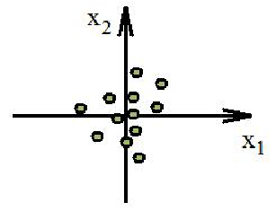
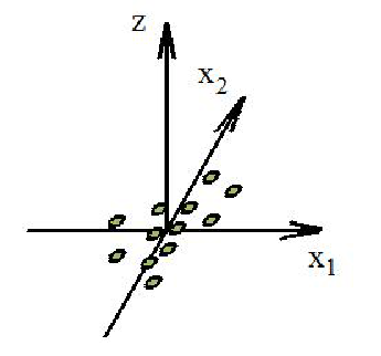
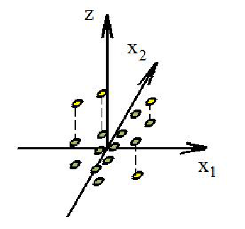
We see that a lift is completely defined by a symmetric matrix : with this matrix given one computes the rest of the coefficients from eq. 3 and then the -coordinates of data points from eq. 2. The last requirement of eq. 1 can be then satisfied by a change in the overall normalization of the -coordinate. In fig. 1 we demonstrate the process of data lifting. In fig. 1a there is an initial distribution of data, in fig. 1b there is a space with a single dimension added, and in fig. 1c there are lifted data points (in order not to abuse the figure we show a lift of few points only).
Having carried out the lift, we may consider various orthogonal rotations in the extended space. Such a rotation will change coordinates of data points and, in particular, their projections onto the subspace . Orthogonal rotations do not change neither first nor second moments provided that they have been normalized. However, the third moment tensor of the lifted distribution will rotate together with data points and its projection on the subspace will change. Therefore we have at this point a tool to change the third moment of the distribution without destroying the first two. We would like to choose a rotation of the lifted distribution in a way that would minimize the third moment of the new distribution in the subspace . It follows from this construction that the coordinates of any new data point in are quadratic functions of its initial coordinates.
Recall that we still have a freedom to choose a symmetric matrix , which defines a lift. In order to get rid of this ambiguity we consider an addition of many such -coordinates, one for every independent component of . There are such components, so we add this amount of dimensions and denote them by . Each dimension is added independently of others in the way described above. At the end we get a distribution which satisfies the following conditions, which generalize the first two of eq. 1 to higher-dimensional case: . In order to have completed a normalization of the second moment (i.e. to provide that ) it remains to normalize the third moment of the -coordinates by means of RX in -dimensional space. With this have been done, we obtain a distribution in the -dimensional space with normalized first two moments. Then we want to rotate it in a way that will cancel a third moment of the projection onto the -dimensional subspace , which we still denote by .
We turn now to a description of a numerical procedure for computing the necessary rotation. It is by no means necessary to compute it this way, one can follow a different route instead. For instance, one can use some kind of Tucker decomposition of the third order tensor, following the ideas of [13, 14], or employ a modification of an Alternating Least Squares algorithm (a commonly used version of it will produce some sign differences in rotation matrices of different tensor dimensions, which is unacceptable).
Denote a third moment of the lifted distribution by , where the indices run over the values of . We endow it with a norm
| (4) |
where the indices in the first expressions run only over the subspace , whereas in the second they run over the whole space, but there appears a matrix which carries out a projection onto .
Consider orthogonal rotations (the orthogonality conditions that they should satisfy are ), under which tensors transform as
| (5) |
Introduce infinitesimal rotations which mix two types of dimensions. A matrix of such a rotation can be written in a block form as
| (6) |
where upper-left corner is of dimension and the lower-right corner is of dimension . The projection matrix introduced above is of the form
| (7) |
A norm of the rotated tensor is
| (8) |
where an explicit form of the matrix is
| (9) |
Then a change in the norm under such a rotation to the first order in is
| (10) |
We see that if we choose to be proportional to
| (11) |
then we achieve the fastest decrease of the norm. Therefore we can carry out a gradient descent computation, where at every step we choose a rotation matrix to be of the form
| (12) |
where is some small parameter. The full rotation matrix is a multiplication of matrices obtained at the intermediate steps. Along this gradient descent flow the following differential equations for components of hold:
| (13) | |||
| (14) | |||
| (15) | |||
| (16) |
with defined in eq. 11. At the final point of the evolution will vanish. Since a pair of indices accepts values, the same amount as does , one can think of the result as a matrix of dimension acting on vectors in - dimensional space (written as ) with vanishing result. If the matrix is non-degenerate then it is possible only if . So the only possibly problematic points in the space of tensors are those at which is a degenerate operator. At these points the first order expansion of the norm is not sufficient; to the first order there is no change in the norm and the question is whether such a point is a local minimum of the norm or it is rather a saddle point or even a local maximum. In the former case the algorithm will get stuck there (if it reaches a vicinity of it), whereas in the latter cases it will escape that point.
An expansion of the norm to the second order in around a point with is
| (17) |
In the last term in this expression there appear components of the tensor, components which did not appear at all in the discussion above. If they are large enough they can in principle make this expression positively definite. From the construction it is clear that these components are related to higher moments of the initial distribution (up to fifth moment). So, if these higher moments are very large the algorithm may not find a rotation that would cancel the third moment. In the next section we discuss some possible approaches to a solution of this problem. However, in all practical situations considered by the author the algorithm converged to 0.
In fig. 2 we present a result of this computation on a simulated two-dimensional data. The data points are initially distributed homogeneously within a triangle , , . In addition, there are four anomalous data points above the diagonal. A coloring of the points is introduced in order to clarify a distortion of the distribution when more and more moments have been normalized. In fig. 2b there is a distribution with first two moments normalized (in other words, the result of RX). The triangle has become an equilateral one (which is more symmetric), but anomalous data points are still not of the biggest norm. In fig. 2c there is a distribution with three first moments normalized. The distribution is almost circular, and the anomalous data points are of the biggest norms.


4 Conclusions and summary
In this paper we described an algorithm for a standardization of the third moment of data distributions and presented an example of its operation. The algorithm consists of two steps:
- 1.
Lift the data by adding dimensions to initial -dimensional space. Values of new coordinates are quadratic functions of initial coordinates.
- 2.
Rotate a new distribution so that in the third moment of the projection onto the horizontal subspace would vanish.
Some remarks here are in order.
Firstly, the author is neither aware of an analytic solution for a rotation that would make the third moment of the projection vanish, nor was he able to solve for it, and therefore had to implement a numeric solution described above. Moreover, as shown in the previous section, there might in principle be situations where the algorithm in its present form will not converge. It is a challenging problem to find such an analytic solution. A knowledge of it can both improve a performance and answer a question of a convergence of the algorithm in all possible situations, a question which is still open (although the algorithm converged in all situations considered by the author).
Secondly, although a numeric search for a rotation mentioned in the previous paragraph takes a certain time, the most lengthy part is a computation of a third moment of the lifted distribution. The author made no essential attempt to optimize this part by, say, implementing a kind of parallel computation. If there is a good way to implement a parallel computation at this stage then the overall performance of the algorithm becomes significantly better.
Despite these two shortcomings, the algorithm is rather fast if a number of dimensions is not too large. For a five-dimensional data of a one million points it works less than a half a minute on a standard PC (a code is written in MATLAB). For large dimensionality the algorithm in the form described above is inapplicable since it requires at intermediate steps an addition of dimensions to data, and their number goes as . Then, however, one can implement a different version of it, where one adds a single dimension at a time and then rotates a distribution so as to minimize a norm of the projection. Then again a dimension is added, etc. In such a version there is no need in large amount of additional memory, but a transformed data is no more a quadratic function of the initial one but will rather be given by some high power functions, with the power being uncontrollable. Similar ideas can be applied to situations with exceptionally large higher moments, where the algorithm discussed above might fail.
5 Acknowledgements
The author is grateful to O. Graubart for fruitful discussions along the whole work.
References
- [1] K. Pearson, “On lines and planes of closest fit to systems of points in space", Philosophical Magazine 2 (6), 559 (1901).
- [2] P. Geladi, B. Kowalski, “Partial least squares regression: a tutorial", Analytica Chimica Acta (1986), 185.
- [3] J.P Benzecri, “L’Analyse des Donne’es. Volume II. L’Analyse des Correspondances", Paris, France: Dunod (1973).
- [4] H.P. Kriegel, P. Kroger, E. Schubert, A. Zimek, “A general framework for increasing the robustness of PCA-based correlation clustering algorithms", Scientific and Statistical Database Management. Lecture Notes in Computer Science 5069 (2008), 418.
- [5] I. Reed and X. Yu, “Adaptive multiband cfar detection of an optical pattern with unknown spectral distribution, IEEE ASSP, vol. 38, no. 10, pp. 17601770, Oct 1990.
- [6] J. D. Carroll, J. Chang, “Analysis of individual differences in multidimensional scaling via an n-way generalization of EckartYoung decomposition", Psychometrika 35 (1970) 283.
- [7] R. A. Harshman, “Foundations of the PARAFAC procedure: Models and conditions for an "explanatory" multi-modal factor analysis", UCLA Working Papers in Phonetics, 16, (1970) 84 pp. (University Microfilms, Ann Arbor, No. 10,085).
- [8] L. R. Tucker, “Some mathematical notes on three-mode factor analysis", Psychometrika 31 (3) (September 1966), 279.
- [9] T. Blaschke, L. Wiskott, “An improved cumulant based method for independent component analysis", Proc. int’l conf. on artificial neural networks, ICANN’02, Madrid, August 2002, in series Lecture notes in computer science, publ. Springer-Verlag, p. 1087.
- [10] T.G. Kolda, B.W. Bader, “Tensor decompositions and applications", SIAM review 51(3), 2009, p. 455.
- [11] Yan-Gang Zhao, Tetsuro Ono, “Third moment standardization for structural reliability analysis", Journal of structural engineering, June 2000, 724.
- [12] E.K. Gnang, A. Elgammal, V. Retakh, “A Spectral Theory for Tensors", arXiv:1008.2923.
- [13] C.A. Andersson, R. Henrion, “A general algorithm for obtaining simple structure of core arrays in -way PCA with application to fluorometric data", Comp. Statistics and Data Analysis, 31 (1999) 255.
- [14] R. Rocci, J.M.F. Ten Berge, “Transforming three-way arrays to maximal simplicity", Psichometrica 67 (3) (2002) 351.