Beyond Random Walk and Metropolis-Hastings Samplers: Why You Should Not Backtrack for Unbiased Graph Sampling
Abstract
Graph sampling via crawling has been actively considered as a generic and important tool for collecting uniform node samples so as to consistently estimate and uncover various characteristics of complex networks. The so-called simple random walk with re-weighting (SRW-rw) and Metropolis-Hastings (MH) algorithm have been popular in the literature for such unbiased graph sampling. However, an unavoidable downside of their core random walks – slow diffusion over the space, can cause poor estimation accuracy. In this paper, we propose non-backtracking random walk with re-weighting (NBRW-rw) and MH algorithm with delayed acceptance (MHDA) which are theoretically guaranteed to achieve, at almost no additional cost, not only unbiased graph sampling but also higher efficiency (smaller asymptotic variance of the resulting unbiased estimators) than the SRW-rw and the MH algorithm, respectively. In particular, a remarkable feature of the MHDA is its applicability for any non-uniform node sampling like the MH algorithm, but ensuring better sampling efficiency than the MH algorithm. We also provide simulation results to confirm our theoretical findings.
Keywords: unbiased graph sampling, random walks, non-reversible Markov chains, semi-Markov chains, asymptotic variance
1 Introduction
Estimating various nodal and topological properties of complex networks such as online social networks (OSNs), peer-to-peer (P2P) networks, and the world wide web (WWW) has recently attracted much attention from research community because of their ever-increasing popularity and importance in our daily life. However, the estimation of network characteristics is a non-trivial task, as these networks are typically too large to measure, making a complete picture of the network hard to obtain and even its size unknown. It is thus infeasible to perform ‘independence sampling’ which obtains uniform node samples (for unbiased estimation) directly and independently from such a large, unknown network. Instead, graph crawling techniques – graph sampling via crawling, have been widely used for that purpose. In particular, random walk-based graph sampling methods (or Markov chain samplers) have become popular, as they are simple and implementable in a distributed fashion and also able to provide unbiased graph sampling, unlike the breadth-first-search (BFS) and its variants leading to unknown bias [12, 20].
In the literature, the most popular random walk-based graph sampling methods are the so-called simple random walk with re-weighting (SRW-rw) [29, 12] and Metropolis-Hastings (MH) algorithm [25, 16, 34, 29, 12, 15]. The former launches a simple random walk (SRW) over a graph , which moves from a node to one of its neighbors chosen uniformly at random, to collect random node samples, followed by a re-weighting process in order to eliminate the bias caused by the non-uniform stationary distribution of the SRW. The other method is to rely on a Metropolis-Hastings random walk (MHRW) crawling over – a random walk achieving a unform distribution constructed by the famous MH algorithm [25, 16], to obtain uniform node samples.
Motivation and Contributions: While the SRW-rw and MH algorithm ensure unbiased graph sampling, the core components – SRW and MHRW, suffer from their slow diffusion over the space, which can in turn lead to poor estimation accuracy. In particular, their fully random nature in selecting the next node, when making a transition, often cause them to go back to the previous node from where they just came. This produces many duplicate samples for a short to moderate time span, thereby reducing estimation accuracy. It is apparently desirable to avoid such backtracking transitions whenever possible, so as to steer them toward ‘unvisited’ places (or to obtain new node samples), as long as such a modification does not affect the unbiased estimation.
However, it is still uncertain how to achieve this at almost no additional cost and whether it really results in better estimation accuracy. We provide affirmative answers for these questions. Specifically, we propose non-backtracking random walk with re-weighting (NBRW-rw) and MH algorithm with delayed acceptance (MHDA), and prove that each of them guarantees not only unbiased graph sampling but also higher efficiency (smaller asymptotic variance of the estimators) than the SRW-rw and the MH algorithm, respectively. A notable feature of our MHDA is its generic purpose: the MHDA is theoretically guaranteed to enhance the standard MH algorithm for constructing a random walk or a Markov chain with any arbitrarily given stationary distribution under the constraints of graph structure. Thus, the MHDA is applied, as ‘a special case’, to construct a random walk crawling over a graph achieving a uniform stationary distribution, leading to higher efficiency than the MHRW while ensuring the unbiased estimation. To the best of our knowledge, this is the first theoretical result to improve, with proven guarantee, both SRW-rw and the MH algorithm for unbiased graph sampling.
Related Work: Very recently, there have been a few attempts to improve the estimation accuracy against the SRW-rw (not the MH algorithm) through multiple dependent random walks [30], a random walk on a weighted graph (with a priori estimate of network information) [20], and the addition of random jumps (to anywhere in the graph) [5]. The corresponding Markov chains are time-reversible, whereas the main kernel of our proposed methods is transforming ‘any’ reversible Markov chain to its related non-reversible chain which avoids backtracking transitions and also achieves the same stationary distribution. Thus, our work is complementary to their approaches.
On the other hand, there is a body of research works across many disciplines for speeding up a random walk, or Markov chain, on a graph in terms of its mixing time, hitting time, and/or cover time. The fastest mixing (reversible) Markov chain on a graph is obtained in [8] with complete knowledge of entire graph. [9, 10] showed that certain ‘lifted’ (non-reversible) Markov chains converge to their stationary distributions faster than their related reversible chain, and [19, 22] subsequently applied this idea to design a fast and efficient average consensus algorithm. It is, however, still unknown how to construct such a ‘lifted’ Markov chain in a distributed or decentralized manner for a general graph.
[3, 7, 17] recently undertook speeding up a SRW based only on local information, but did not provide any direct implication to the unbiased graph sampling. As the MH algorithm is the most popular method of Markov Chain Monte Carlo (MCMC) simulations or samplers, it has been an active research topic to improve the MH algorithm in terms of the sampler performance (asymptotic variance) in the MCMC literature (e.g., [26, 14, 35]). However, most works toward more efficient MCMC samplers (including [26, 14, 35]) do not take into account graph-topological constraints in that transition from node to is allowed only when they are neighbors of each other, and thus cannot be directly applicable to unbiased graph sampling.
Organization: The rest of the paper is organized as follows. We first provide an in-depth overview on generic Markov chain samplers for unbiased graph sampling in Section 2, and then briefly review the SRW-rw and MH algorithm in Section 3. In Section 4, we present a general recipe for the transformation of a time-reversible Markov to its related non-reversible Markov chain, which forms a common building block for our proposed NBRW-rw and MHDA. We then explain the details of the NBRW-rw and MHDA, and provide relevant analysis. In Section 5, we provide simulation results obtained based on real graphs to support our theoretical findings. We finally conclude in Section 6.
2 Background on Markov Chain Samplers
2.1 Unbiased Graph Sampling
Consider a connected, undirected graph with a set of nodes (vertices) and a set of edges . We assume that . We also assume that the graph has no self-loops and no multi-edges. Let be the set of neighbors of node , and be the degree of node .
Unbiased graph (or node) sampling, via crawling, is to consistently estimate nodal or topological properties of a target graph ** * A target graph for sampling may be time-varying due to node join/leave, which is beyond the scope of this paper. (e.g., an overlay network or an OSN) based upon uniform node samples obtained by a random walk (or possibly multiple random walks) crawling over the graph . The goal here is to unbiasedly estimate a proportion of the nodes with a specific characteristic. Thus, the unbiased, uniform graph sampling is, in principle, developing a random walk-based “estimator” or a Markov chain sampler for the expectation of any given, desired function with respect to a uniform distribution, i.e.,
| (1) |
where . Note that a nodal (or topological) characteristic of interest can be specified by properly choosing a function . For example, for a target graph , if one is interested in estimating its degree distribution (say, ), then choose a function such that for , i.e., if , and otherwise.
We below review a basic Markov chain theory which serves as the mathematical foundation for unbiased graph sampling via a (Markovian) random walk crawling over a graph . Define a random walk or a finite discrete-time Markov chain on the nodes of the graph with its transition matrix in which
and for all . Each edge is associated with a transition probability with which the chain (or random walk) makes a transition from node to node . We allow the chain to include self-transitions, i.e., for some , although has no self-loops. Clearly, for all (). We then assume that the Markov chain is irreducible, i.e., every node in is reachable in finite time with positive probability, such that the chain has a unique stationary distribution .
For any function , define an estimator
| (2) |
for the expectation of the function with respect to which is given by
| (3) |
Then, the following Strong Law of Large Numbers (SLLN) (a.k.a., ergodic theorem) has been a fundamental basis for most of the random walk-based graph sampling methods in the literature [34, 29, 12, 15, 30, 5, 20], and more generally, MCMC samplers [28, 26, 35, 18, 31, 27].
Theorem 1
The SLLN ensures that the estimator based on any finite, irreducible Markov chain with the same can serve as a valid and unbiased approximation of . In particular, the two popular random walk-based graph sampling methods (or two different Markov chain samplers for unbiased graph sampling) in the networking literature – SRW-rw [29, 12] and MH algorithm [34, 29, 12, 15] are built upon the SLLN to asymptotically guarantee the unbiasedness of their estimators for . We will review in detail these two graph sampling methods in Section 3.
2.2 Central Limit Theorem and Asymptotic Variance
For a given graph , there are potentially many (finite) irreducible Markov chains (or different random walks) preserving the same stationary distribution , all of which can be used to obtain asymptotically unbiased estimates of , and also of , together with proper re-weighting if . One important question would then be how to compare these ‘competing’ Markov chains, or rather, which one is ‘better’ or more efficient than the others as a Markov chain sampler for unbiased graph sampling.
Mixing time can perhaps be a criterion to compare several irreducible, aperiodic Markov chains, all with the same stationary distribution. The mixing time captures the notion of the speed of convergence to the stationary distribution, and is typically defined via the total variation distance: for an irreducible, aperiodic Markov chain with its transition matrix and stationary distribution , the mixing time can be written as
where the total variation distance is defined by . Here, denotes the -step transition probability from node (state) to subset , and . The mixing time has been actively studied in the literature, especially for irreducible, aperiodic, time-reversible†† † If the Markov chain satisfies the reversibility condition (or detailed balance equation), i.e., for all , then the chain is called time-reversible. Markov chains (e.g., [8, 21]). In particular, it is now well known that the mixing time of such a Markov chain (or the asymptotic rate of convergence to its stationary distribution) is mainly governed by the second largest eigenvalue modulus (SLEM) – the second largest eigenvalue in absolute value, of its transition matrix, and smaller SLEM leads to smaller (faster) mixing time [8, 21].
If the speed of convergence to the stationary distribution is a primary concern, then the mixing time is surely the right metric to compare different Markov chains with the same stationary distribution. However, this is not the case for the unbiased graph sampling. Random walk-based graph sampling methods typically adopt an initial burn-in period over which (initial) sampled values are discarded to get rid of the dependence on the initial position of a random walk [12]. After such a burn-in period, the Markov chain (or random walk) will be close to its stationary regime (well mixed), but many samples are still yet to be obtained from this point onward. Therefore, the primary concern should be, instead, the efficiency of the estimator in deciding how many random samples are required to achieve a certain accuracy of in regard to (and eventually to after proper re-weighting if necessary).
To that end, we define by the asymptotic variance of the estimator based on an irreducible Markov chain with its stationary distribution , which is given by
| (4) |
for any function with , where the initial position (state) is drawn from the stationary distribution , i.e., . Note that the asymptotic variance is, in fact, independent of the distribution of the initial state [28, 31]. We below explain how effective the asymptotic variance can be, through its connection to the Central Limit Theorem (CLT), in measuring the performance of the estimator .
Suppose first that the random samples are i.i.d. and drawn directly from . Then, the standard Central Limit Theorem (CLT) says that
where denotes convergence in distribution and is a Gaussian random variable with zero mean and variance . That is, the distribution of is asymptotically normal. For sufficiently large , we also have
which allows us to identify an approximate confidence interval for . For instance, for sufficiently large , we can be confident that is approximately between and . This clearly demonstrates the importance of the asymptotic variance in conjunction with the CLT in assessing the accuracy of the estimator .
Not only for the above case with i.i.d. samples, the CLT holds also for Markov chains, as given below.
Theorem 2
Note that Theorems 1–2 (SLLN and CLT) do not require any assumption of aperiodicity [31]. However, for simplicity, we do not consider periodic Markov chains in our analysis throughout the paper. In addition, we focus on bounded functions (and thus ), which is typical in graph sampling applications.
As shown above for i.i.d. samples, the CLT allows one to evaluate the asymptotic variance in order to decide approximately how many (correlated) samples are required to achieve a certain accuracy of the estimator . Hence, the asymptotic variance has been an important criterion to rank the efficiency among competing Markov chains with the same for the MCMC samplers [28, 26, 35, 18, 31, 27], although quantifying may not be easy. In particular, by noting that the asymptotic variance is independent of any initial distribution for which the CLT holds, the efficiency ordering over competing Markov chains with the same (the smaller the asymptotic variance, the better the estimator performance) is still in effect even when the competing Markov chains are already in their stationary regimes (already ‘mixed’). Observe that from , for all (the chain is in the stationary regime), and thus (4) becomes
| (5) |
where denotes the covariance between and . That is, even if the competing Markov chains are already in their stationary regimes, the correlation structure over random samples given by each of these Markov chains can vary and significantly affect their asymptotic variances. Observe that reducing the temporal correlation over random samples can lead to smaller asymptotic variances. This intuition can be leveraged to improve the existing Markov chain samplers for unbiased graph sampling.
Motivated by the effectiveness of the asymptotic variance with its connection to the CLT, in this paper, we consider the asymptotic variance as a primary performance metric, and develop two random walk-based graph sampling methods, each of which guarantees the unbiased graph sampling with smaller asymptotic variance than its corresponding counterpart in the current networking literature. Before going into details, we next briefly review the existing two random walk-based graph sampling methods.
3 Random Walk-based Graph Sampling
3.1 Simple Random Walk with Re-weighting
We first review the SRW-rw, a.k.a., respondent-driven sampling [33], which has been recently used in [29, 12] for unbiased graph sampling. This method operates based upon a sequence of (correlated) random samples obtained by a SRW, together with a proper re-weighting process to ensure the unbiased sampling. It is essentially a special case of the importance sampling (a Monte Carlo method) applied for random samples generated by a Markov chain [6, 23, 13]. While there are similar variants of such method (e.g., [24]), the main idea behind them is still to correct the sampling bias caused by the stationary distribution of the SRW.
Consider a SRW on that moves from a node to one of its neighbors chosen uniformly at random (u.a.r.). Specifically, let be the Markov chain representing the sequence of visited nodes by the SRW, with its transition matrix given by
| (6) |
It is well known that is irreducible, and reversible with respect to a unique stationary distribution for which [2].
Suppose that there are random samples from the SRW. Then, for a function of interest , choose a weight function such that
Observe that from the SLLN in Theorem 1, as ,
and thus the estimator is unbiased for . However, this estimator itself is not practical, since and are typically unknown a priori. Instead, another estimator is often used as an unbiased estimator for . Indeed, Theorem 1 asserts that and converge to and 1 almost surely, as , respectively. This yields
Hence, the estimator can be made in such a way that we need to know only up to a multiplicative constant. That is, if we set , , then the estimator remains intact, and is more practical as an unbiased estimator for . Throughout this paper, we refer to the estimator with () as the unbiased estimator for in the SRW-rw [29, 12].
As an example, for a target graph , choose a function such that for in order to estimate the degree distribution . Then, for any given ,
implying that the estimator yields a valid unbiased estimate of .
3.2 Metropolis-Hastings Algorithm
The MH algorithm [25, 16] was developed to construct a transition matrix of a time-reversible Markov chain with a given, desired stationary distribution . Here, we only discuss the MH algorithm under the topological constraints of a graph in that transition from node to is allowed only when they are neighbors of each other. The MH algorithm is defined as follows. At the current state of , the next state is proposed with a proposal probability , which is a state transition probability of an arbitrary irreducible Markov chain on the state space , where if and only if , and for all (). Let be a proposal (transition) matrix. The proposed state transition to is accepted with an acceptance probability
| (7) |
and rejected with probability in which case . Thus, the transition probability becomes, for ,
| (8) |
with , which ensures that is reversible with respect to . Note that the uniqueness of is granted due to the irreducibility of (so is ) and the finite state space.
The MH algorithm, in addition to its popular applications for MCMC simulation, has been also widely used as a means for unbiased graph sampling [34, 29, 12, 15]. Specifically, the MH algorithm has been applied to construct a MHRW on achieving a uniform stationary distribution, i.e., . This is done with transition probabilities of a SRW as the proposal probabilities, i.e., if and , otherwise. The resulting transition probability of the MHRW on becomes
| (9) |
and . Thus, is reversible with respect to , implying that for any function , the estimator based upon random samples by the MHRW is unbiased for . This version of MH algorithm is summarized in Algorithm 1, where denotes the location of the MHRW at time , and denotes the degree of node . Here, can be arbitrarily chosen.
Remark 1
It is worth noting that the MH algorithm (Algorithm 1) does not need to know the self-transition probabilities explicitly, nor does it require all the neighbors’ degree information of the current node at each time . Instead, only the degree information of the randomly chosen neighbor is enough for making decision whether or not to move to .
Recall that the above unbiased estimators are based on random, consecutive samples obtained under SRW or MHRW, respectively. Observe that the SRW, currently at node at time can ‘backtrack’ to the previously visited node with probability , i.e., , trapping the SRW temporarily in a local region. The situation can be worse for the regions in which nodes have small degrees (so higher chance of backtracking). Similarly, the MHRW at node can also backtrack to the previously visited node after staying at node for some random time. This slow ‘diffusion’ of SRW/MHRW over the space can, in turn, lead to highly duplicated random samples for a short to moderate time duration, thereby increasing the variance of the unbiased estimators. Recall that the asymptotic variance in (5) involves covariance terms . Thus, it would be beneficial for both SRW and MHRW (or precisely, their variants) to avoid backtracking to the previously visited node up to the extent possible in order to reduce the temporal correlation over random consecutive samples, while maintaining the same stationary distribution so that the aforementioned mathematical framework for the unbiased estimation remains intact. Thus motivated, for the rest of this paper, we investigate how to achieve this at almost no additional cost, and rigorously prove that our proposed sampling methods give smaller (no worse) asymptotic variance than the SRW (with re-weighting) and MHRW-based ones, respectively.
4 Avoid Backtracking To Previously Visited Node
In this section, we propose two random walk-based graph sampling methods – (i) non-backtracking random walk with re-weighting and (ii) MH algorithm with delayed acceptance, each of which theoretically guarantees unbiased graph sampling with smaller asymptotic variance than the SRW-rw and the (original) MH algorithm, respectively. In particular, our proposed sampling methods require almost no additional cost, or more precisely, just remembering where the underlying random walk came from, when compared to the conventional methods. The reasoning behind the improvement of asymptotic variance is to modify each of SRW and MHRW, when making a transition from the current node to one of its neighbors, to reduce bias toward the previous state (one of the neighbors of the current node), while maintaining the same stationary distribution. Note that such directional bias breaks the time-reversibility of the SRW and MHRW. Thus, a common building block for our proposed sampling methods will be, for a given reversible Markov chain with its stationary distribution , to construct a non-reversible Markov chain preserving the same while avoiding (to the extent possible) transitions that backtrack to the state from which the chain just came. Our challenge here is to construct such a non-reversible chain with only one-state memory and theoretical guarantee for higher efficiency (smaller asymptotic variance). In what follows, we first explain a basic setup for this transformation and several relevant issues, and then present the details of our proposed methods.
4.1 From Reversible To Non-reversible Chains
Consider a generic random walk on , or a finite, irreducible, time-reversible Markov chain , with its transition matrix and stationary distribution . Our goal here is to construct its related new random walk or a finite, irreducible, non-reversible Markov chain with the same which avoids backtracking to the previously visited node, which in turn produces a smaller asymptotic variance than the original reversible chain. An important requirement is that this transformation should be done at no additional cost and in a distributed manner. It is worth noting that there have been other works [9, 10] showing that certain non-reversible Markov chains or lifted Markov chains mix substantially faster than their related reversible chains. While this concept has been also applied to design a fast and efficient average consensus algorithm [19, 22], it is still unknown how to construct such a non-reversible chain or lifted Markov chain in a fully distributed or decentralized fashion, not to mention how to do so for any arbitrarily given target stationary distribution .
A general recipe for constructing a non-reversible Markov chain in an augmented state space: Let , , be the location of a new random walk at time . At the current node , the next node is decided based upon not only the current node but also the previous node so as to avoid backtracking. Due to the dependency (memory) to the previous node, itself cannot be a Markov chain on the state space , regardless of the choice of transition matrix. This walk, however, can still be made Markovian on an augmented state space instead, defined by
| (10) |
with , and for . For notational simplicity, let denote state . Note that . It is also possible that for some . A similar interpretation of a weighted random walk (or a reversible Markov chain) on the augmented state space can be also found in [2, Ch.3], although its purpose is not for the construction of a related non-reversible chain.
Let be the transition matrix of an irreducible Markov chain on the state space . Here, by definition, for all . If the unique stationary distribution of the chain is given by
| (11) |
implying that from the reversibility of the original chain , then the probability of the new random walk being at node in the steady-state is the same as for all (the stationary distribution of the original reversible chain ). To see this, note that
| (12) |
where the first equality follows from , . In particular, for any original function of interest , choose another function such that , and observe
Then, the SLLN in Theorem 1 gives
| (13) |
i.e., is a valid unbiased estimator for . We thus define, for any given function ,
| (14) |
to be clearly distinguished from in (1) defined based on the original chain , while and are both unbiased estimators for . In addition, the CLT in Theorem 2 implies
| (15) |
where denotes the asymptotic variance of (and also of ). Throughout the paper, we use the prime symbol (′) for any notation related to a newly defined process (e.g., ) to differentiate it from its counterpart defined on the original process (e.g., ).
While there are infinitely many different transition matrices leading to the unbiased estimator for , our primary goal is, at (almost) no additional cost and in a distributed manner, to find a transition matrix that also guarantees smaller asymptotic variance. Under a rather restricted setting, R. Neal gave a partial answer to this in [27] saying that less backtracking (rendering the resulting Markov chain non-reversible) can result in a smaller asymptotic variance. We restate his finding below.
Theorem 3
[27, Theorem 2] Suppose that is an irreducible, reversible Markov chain on the state space with transition matrix and stationary distribution . Construct a Markov chain on the state space with transition matrix in which the transition probabilities satisfy the following two conditions: for all with ,
| (16) | ||||
| (17) |
Then, the Markov chain is irreducible and non-reversible with a unique stationary distribution in which , . Also, for any function , the asymptotic variance of is no greater than that of , i.e., .
Remark 2
The condition in (16) ensures that the resulting transition matrix is stationary with respect to in (11) and, in turn, leads to the unbiased estimator for . Together with this condition, the condition in (17) – less backtracking to the previously visited node, brings out the improvement of asymptotic variance.
Theorem 3 is quite versatile and provides a guideline on how to choose the transition matrix of a Markov chain leading to smaller asymptotic variance, and thus will play an essential role in developing our graph sampling methods and subsequent analysis. Despite this large degree of freedom, it is still uncertain how to choose such a transition matrix at no additional cost. While R. Neal suggested a procedure to find , it generally poses significant cost, especially for improving the MH algorithm, as admitted in [27]. (See pp. 9–10 therein.) Recall that the MH algorithm (Algorithm 1) for MHRW only needs the degree information of a randomly chosen neighbor of the current node to decide whether or not to move , as mentioned in Remark 1.‡‡ ‡ More generally, in the MH algorithm with any proposal matrix , it is often unnecessary to know self-transition probabilities explicitly, or does not require summing the probabilities of rejection for all possible proposals just to compute . However, the procedure by R. Neal necessitates the explicit knowledge of all ’s [27]. That is, the corresponding modified MHRW would require all the neighbors’ degree information of the current node at each time in order to choose the next node . Imagine such modified MHRW crawling over an OSN (say, Facebook) and located at a certain user’s page. To simply decide where to go, the walk would have to visit all his/her friends’ pages first and collect all their degree information (i.e., the number of friends) before making decision to move. This is clearly impractical for our graph sampling purpose. Therefore, in this paper, we set out to develop our own graph samplers with higher efficiency without any such overhead, by leveraging Theorem 3 as a building block.
4.2 Non-backtracking Random Walk with Re-weighting
We first introduce non-backtracking random walk with re-weighting (NBRW-rw) that ensures unbiased graph sampling, and then prove that NBRW-rw guarantees a smaller asymptotic variance than SRW-rw. The non-backtracking random walk (NBRW) is a discrete-time random walk which ‘never’ backtracks (thus named non-backtracking) to the previous node (whenever possible) while preserving the same stationary distribution as that of a SRW. Thus, the proposed sampling method is to use an NBRW, instead of a SRW, to collect a sequence of samples by crawling over a target , and at the same time, to employ the same re-weighting process as is done for SRW in order to eliminate sampling bias induced from its non-uniform stationary distribution.
Consider an irreducible, reversible Markov chain (a sequence of visited nodes) by the SRW with its transition matrix given by (6), and stationary distribution , . Then, the NBRW is defined as follows. A (discrete-time) random walk at the current node with moves to the next node , chosen u.a.r. from the neighbors of node except the previous node . If the current node has only one neighbor (), the walk always returns to the previous node . Figure 1 depicts this non-backtracking nature of the NBRW in its transitions over the nodes of . Here, an initial position of the NBRW can be arbitrarily chosen. The NBRW initially moves from the initial position to one of its neighbors with equal probability due to the absence of its ‘previous node’, and then proceeds as defined above thereafter.

Let , , be the location of an NBRW. As before, we construct a Markov chain with its transition matrix given by, for all with (),
| (18) |
implying that . Also, for any with . All other elements of are zero. Clearly, satisfies the conditions in (16)–(17). From Theorem 3, the Markov chain is irreducible and non-reversible with a unique stationary distribution
| (19) |
That is, the probability of the NBRW being at node in the steady-state is the same as . See (12). From (13)–(14) and Theorem 3, we also know that for any given function of interest, and are both unbiased estimators for , and the asymptotic variance of (based on the random samples by the NBRW) is no larger than that of (by the SRW), i.e., .
However, both unbiased estimators and are for , not . It is unclear whether such improvement for the asymptotic variance remains true even after a proper re-weighting to obtain unbiased samples. As explained in Section 3.1, the SRW-rw is to use the estimator with in order to consistently estimate . Since the stationary distribution of the NBRW remains the same as that of the SRW, we can also use the estimator with the same weight function , as a valid approximation of . Let and denote the asymptotic variances of the estimators and , respectively. To proceed, we need the following.
Theorem 4 (Slutsky’s theorem)
[4, pp.332]
Let and be the sequences of random variables.
If , and converges in
probability to a non-zero constant , then .
Now we state our main result.
Theorem 5
For any function , the asymptotic variance of is no larger than that of , i.e., , where the weight function is given by , .
Proof: Since the estimator remains invariant up to a constant multiple of , without loss of generality, we can set . For any given , observe that
| (20) |
Define another function such that
implying . Then, from Theorems 1 and 2, we have, as ,
Since almost sure convergence implies convergence in probability [4], by Slutsky’s theorem, from (20), we have
Together with (13) and (15), following the same lines above, we similarly have
Hence, for a given , the asymptotic variance of the estimator is nothing but . Similarly, . Therefore, since Theorem 3 says that for any function , , we also have . That is, the asymptotic variance of is no larger than that of .
Remark 3
In [3], the NBRW was originally considered for regular graphs with , and shown to lead to faster mixing rate (i.e., faster rate of convergence to its stationary distribution) than that of the SRW. In contrast, for any general (connected, undirected, not necessarily regular) graph , we show that the NBRW-rw ensures not only the unbiased graph sampling but also smaller asymptotic variance than the SRW-rw.
4.3 Metropolis-Hastings Algorithm with Delayed Acceptance
We turn our attention to improving the MH algorithm. For any given, desired stationary distribution , we propose Metropolis-Hastings algorithm with delayed acceptance (MHDA), which theoretically guarantees smaller asymptotic variance than the (generic) MH algorithm with proposal matrix that constructs a reversible Markov chain with arbitrary . In particular, we demonstrate that MHDA can be applied, as a special case, to construct a (non-Markovian) random walk on a graph which not only achieves a uniform stationary distribution for unbiased graph sampling, but leads to higher efficiency than MHRW by the MH algorithm (Algorithm 1). We emphasize that the only additional overhead here is remembering the previously visited node (one of the neighbors of the current node) from which the random walk came.
Interpreting a reversible MH Markov chain as a semi-Markov chain: Consider an irreducible, reversible Markov chain by the MH algorithm with its transition matrix given by (8), and any arbitrarily given target stationary distribution . Recall that the MH algorithm is nothing but a repetition of proposing a state transition with proposal probability that is then accepted with an acceptance probability in (7) or rejected otherwise. Observe that the process , after entering into state (node) , stays at state for a geometrically distributed time duration with mean , and then moves to another state . Formally, define a Markov chain with its transition matrix given by, for ,
| (21) |
with . It is not difficult to see that the chain is irreducible, and reversible with respect to a unique stationary distribution , given by
Also, we define a function such that, for ,
| (22) |
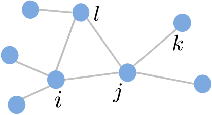
and define a sequence for which depends solely on and is geometrically distributed with parameter . It thus follows that , . The process can now be interpreted as a semi-Markov chain with embedded Markov chain and respective sojourn times . Suppose that the random walk by the MH algorithm (or the process ) enters node of a graph , depicted in Figure 2, at time (). If we consider a sample path , then we have corresponding sequences and . Note that the standard definition of a semi-Markov process allows the sojourn time to depend on both and (and so we are dealing with a special case). From the theory of semi-Markov processes (e.g., [32]), one can easily recover the stationary distribution as
| (23) |
The above interpretation has been similarly given in the MCMC literature [23, 11]. In particular, it is known that, for any given function ,
| (24) |
converges almost surely to , as , and thus is also an unbiased estimator for [23]. This definition of enables more tractable analysis on its asymptotic variance, denoted as , by connecting it to its counterpart in the importance sampling for Markov chains [23, 11]. Note that for sufficiently large (also ), the (original) unbiased estimator can be written as plus some negligible term (after setting the same initial point ), because it is always possible to find such that . Also, in the limit , and are the same. We thus focus on estimators in the form of in our subsequent analysis.
Consider a sequence of pairs . From the success in the NBRW-rw, one may ask what if the reversible embedded Markov chain is replaced by a related stochastic process , or more precisely, a non-reversible Markov chain on the augmented state space , which avoids backtracking transitions to the extent possible, while preserving the same stationary distribution . Another question can be whether this transformation guarantees that the estimator in (24) based on remains unbiased for and also have higher efficiency than the original one. Our answer is in the affirmative, and this is the reasoning behind the improvement of our proposed MHDA over the standard MH algorithm. We stress here that, in contrast to the NBRW, backtracking transitions in the process should be avoided only up to the extent possible§§ § If is made purely non-backtracking just like we did for NBRW, then we lose unbiasedness for the resulting MH-based estimator in general. so as to maintain the arbitrarily given original stationary distribution . Thus, the extension from the MH algorithm to our proposed MHDA becomes necessarily more involved than the case of NBRW.
Description of MHDA: Let , , be the position of a random walk (or the state of a stochastic process). We also define the augmented state space in (10) based on the reversible embedded Markov chain , where and so for all .
MHDA is described as follows. Suppose that node is the previous node from which the walk came. MHDA first operates just like the MH algorithm. At the current node (state) , the next node is proposed with probability (). Then, the proposed transition to is accepted with probability in (7), and rejected with probability in which case . Here, in contrast to the MH algorithm, MHDA renders the accepted transition to temporarily pending, and applies another procedure to proceed with the actual transition to .¶¶ ¶ If the transition to was accepted after a proposal with , then the MHDA accepts the transition as in the MH algorithm without any further action.
Specifically, for the accepted transition to , if , then the ‘actual’ transition takes place, i.e., , which happens with probability as in the MH algorithm. On the other hand, if , then the transition to node is delayed (thus named ‘delayed acceptance’). The next node is again proposed with another proposal probability , which is a transition probability of an arbitrary Markov chain on the state space , where for all , and if and only if . The (second) proposed transition to is accepted with another acceptance probability , and rejected with probability in which case (backtracking occurs). That is, transition probability in the MH algorithm is leveraged to create another transition opportunity from to in the MHDA. So, the transition from to occurs with larger probability than the MH algorithm (w.p. ). This is also illustrated in Figure 3 where the thickness of arrows represents the corresponding transition probabilities from node to other node (including self-transition). The new acceptance probability will be specified shortly.


In summary, under MHDA, the walker stays at each node for the same random amount of time as it would be under the MH algorithm, while reducing the bias toward the previous node when making transitions to one of its neighbors.
Analysis of MHDA: Let , , be the sequence of nodes visited by the walk, which moves over according to the MHDA. The process is clearly different from the reversible, embedded Markov chain for the MH algorithm. Also, let , , be the respective sojourn time at node . Note that the MHDA behaves differently from the MH algorithm (performs the additional procedure) only when a proposed transition from node to node (occurring with probability ) is accepted with probability in the MH algorithm. Thus, is also geometrically distributed with parameter . See (22) for . That is, given that , the sojourn times and have identical distributions. Therefore, the MHDA, similar to the MH algorithm, can be also characterized by a sequence of the pairs . As an example, if the random walk by the MHDA (or the process ) enters node in Figure 2 at time () and , then we consequently have and . We define, for any given ,
| (25) |
We prove below that converges almost surely to , implying that is an unbiased estimator for . We also prove that, after showing the CLT holds for , the asymptotic variance of , denoted as , is smaller than its counterpart for the MH algorithm.
To this end, we first explain how to properly choose the new acceptance so that the process has the same stationary distribution as that of the reversible embedded chain , while, at the same time, the process reduces backtracking transitions. Instead of the process , we deal with its related non-reversible Markov chain defined on the augmented state space by consulting the general recipe for this purpose in Section 4.1. Recall the state space in (10) obtained from the transition matrix of the chain . We define for , and to be the transition matrix of a Markov chain . For instance, consider a sample path in the above example. We have . If the chain has a unique stationary distribution given by
| (26) |
implying that from the reversibility of the embedded chain , then the steady-state probability of the process being at node is the same as for all . From the description of MHDA, observe that, for all with (),
| (27) |
while , as is also shown in Figure 3(b). Note that specifies the next node of the random walk by MHDA, given that the walk has to move from the current node to one of its neighbors (its sojourn time is over). Thus, and are used here instead of and , respectively. In addition, for any with , we have , , since (due to the stochastic matrix ) and which is shown below.
Among many possible choices for the acceptance probability in the MHDA, we have the following.
Proposition 1
Proof: See Appendix A.
From Theorem 3 and Proposition 1, the Markov chain with its transition matrix as in (27) and (28), is irreducible and non-reversible with a unique stationary distribution in (26). This also implies that the process has the same stationary distribution , as explained before. We now present our main result.
Theorem 6
Consider a given, desired stationary distribution . Under the MHDA with any given and its corresponding in (28), for any given function , as , converges almost surely to , and also the asymptotic variance of is no larger than that of , i.e., .
Proof: See Appendix B.
An application of MHDA for unbiased graph sampling: We explain how MHDA can be applied for unbiased graph sampling applications. In particular, we present how to construct a (discrete-time) random walk by MHDRA, named Metropolis-Hastings Random walk with Delayed Acceptance (MHRW-DA), on that achieves the uniform stationary distribution, i.e., . The MHRW-DA here operates as an extension of Algorithm 1 with the following choice of : for all with (),
| (29) |
implying that . Also, for any with . All other elements are zero. While is the same as the transition matrix of NBRW, a ‘Metropolizing’ step, which is done with in (28), must follow in order to ensure that the stationary distribution is uniform and the resulting estimator is unbiased. In other words, in (28) becomes
This version of the MHDA is summarized in Algorithm 2, where is the location of MHRW-DA at time and indicates the previous node from which the MHRW-DA came (). Here, can be chosen arbitrarily. Since there is no notion of ‘previous node’ at time , MHRW-DA initially behaves the same as MHRW until it moves from the initial position to one of its neighbors, and then proceeds as described in Algorithm 2 thereafter.
Theorem 6 states that the MHDA works for any given stationary distribution , while allowing us to freely choose the new proposal probabilities as desired. Thus, Algorithm 2 for MHRW-DA is nothing but a ‘special case’ of the MHDA. Theorem 6 asserts that MHRW-DA produces unbiased samples with higher efficiency than the corresponding MHRW (Algorithm 1). Again, we emphasize that the only additional overhead for MHRW-DA, compared to the MHRW, is remembering where it came from, . Note that the degree of the previous node is already known and can easily be retrieved, while the degree information of another randomly chosen neighbor is also necessary anyway even in the MH algorithm (to decide whether or not to move there).
5 Simulation Results
In this section, we present simulation results to support our theoretical findings. To this end, we use the following real-world network datasets [1]:
- •
AS-733 – an undirected graph of autonomous systems (ASs) composed of 6474 nodes and 13233 edges, where nodes represent ASs and edges exist according to AS-AS peering relationships.
- •
HEP-TH – a collaboration network among authors who submit papers to High Energy Physics-Theory category in the e-print arXiv, forming an undirected graph with 9877 nodes and 51971 edges, where nodes represent authors and edges exist between authors if coauthoring a paper.
- •
Road-PA – a road network of Pennsylvania, forming an undirected graph with 1088092 nodes and 3083796 edges, where nodes represent intersections and endpoints and edges represent the roads connecting them.
- •
Web-Google – a directed web graph with 875713 nodes and 5105039 edges, where nodes represent web pages and directed edges represent hyperlinks between them. For our simulation, we use an undirected version of this web graph.
To ensure graph connectivity, we also use the largest connected component (LCC) of each graph, where the LCC sizes of the AS-733, HEP-TH, Road-PA, and Web-Google graphs are 6474, 8638, 1087562, and 855802, respectively. Here, the average degrees of AS-733, HEP-TH, Road-PA, and Web-Google graphs are 4.09, 5.75, 2.83, and 10.03, while their maximum degrees are 1459, 65, 9, and 6332, respectively.
As a test case, we consider the estimation of the degree distribution of each graph – (pdf) and (ccdf), to evaluate and compare our proposed NBRW-rw and MHRW-DA (MHDA in Algorithm 2) against SRW-rw and MHRW (MH algorithm in Algorithm 1), respectively. As mentioned before, to estimate , we just need to choose a function , , for the corresponding estimators. Similarly, we choose for . To measure the estimation accuracy, we use the following normalized root mean square error (NRMSE) [5, 30, 20], , where is the estimated value out of samples and is the (ground-truth) real value. ( from unbiasedness.) In all simulations, an initial position of each random walk is drawn from its stationary distribution as similarly used in [5], unless otherwise specified. In practical implementations, one can employ a ‘burn-in’ period to drive the random walk close to its steady-state [12]. Each data point reported here for AS-733 and HEP-TH graphs is obtained from independent simulations, while, for Road-PA and Web-Google graphs, the data points are based on and simulations, respectively.


We first present the simulation results for AS-733 graph whose ‘actual’ degree distribution is almost a ‘power-law’ as depicted in Figure 5 (insets). Figure 4 shows that NBRW-rw (resp. MHRW-DA) outperforms SRW-rw (resp. MHRW) in terms of the required number of samples (cost) to achieve the same level of estimation error when estimating , as expected from our theoretical results. Here, the NBRW-rw (resp. MHRW-DA) brings out about 35% (resp. 14%) cost saving on average, when compared to the SRW-rw (resp. MHRW). In addition, we plot, in Figure 5, the NRMSE ratio of SRW-rw (resp. MHRW) to the case of NBRW-rw (resp. MHRW-DA) for every degree when estimating with samples. It clearly shows the improvement of our proposed methods for each degree (all data points are above one). We also provide the NRMSE curve (with its ratio), in Figure 6, for the comparison between NBRW-rw (resp. MHRW-DA) and SRW-rw (resp. MHRW) when estimating with samples, which is again clearly consistent with our theoretical findings. In addition, we conduct another simulation to see the impact of non-stationary start for each random walk on the sampling accuracy, for which an initial position of each SRW and NBRW is drawn from a uniform distribution, while the initial position for MHRW and MHRW-DA is chosen with a probability proportional to node degree. Under this setting, we measure NRMSE of the estimator of , and observe that NBRW-rw and MHRW-DA still outperform SRW-rw and MHRW, respectively, as shown in Figure 7. Note that there is not much difference between the stationary start and non-stationary start cases. (See Figures 4 and 7.)


We next provide the simulation results for HEP-TH graph whose actual degree distribution is close to exponential as depicted in Figure 9 (insets). As before, Figure 8 demonstrates that NBRW-rw and MHRW-DA surpass SRW-rw and MHRW for the estimation of , respectively. Specifically, the NBRW-rw (resp. MHRW-DA) saves, on average, about 22% (resp. 12%) of the required number of samples to attain the same level of estimation accuracy, which compared to the SRW-rw (resp. MHRW). Also, Figure 9 shows the NRMSE ratio of SRW-rw (resp. MHRW) to the case of NBRW-rw (resp. MHRW-DA) for every degree for the estimation of with samples, while Figure 10 depicts the NRMSE curve (with its ratio) when estimating with samples. Both results are again in good agreement with our theoretical results. Moreover, after repeating the same experiment for the non-stationary start as above, we observe that the improvement from NBRW-rw and MHRW-DA remains preserved, as shown in Figure 11.
We also present the simulation results for Road-PA graph in which every node has small degree, ranging from 1 to 9, and the actual degree distribution (pdf) is given in Figure 13 (inset). As seen from Figure 12, SRW-rw (resp. MHRW) requires more than twice larger samples than the case of NBRW-rw (resp. MHRW-DA) to attain the same level of accuracy for the estimation of . Specifically, the NBRW-rw and MHRW-DA leads to about 60% and 54% cost saving on average. Also, as before, Figure 13 shows the NRMSE ratio of SRW-rw (resp. MHRW) to the case of NBRW-rw (resp. MHRW-DA) for every degree when estimating with samples, and Figure 14 depicts the NRMSE curve (with its ratio) for the estimation of with samples, which are all in good agreement with our theoretical findings. In addition, Figure 15 demonstrates that such considerable performance improvement of NBRW-rw (resp. MHRW-DA) over SRW-rw (resp. MHRW) still prevails for the case of non-stationary start. We observe that the NBRW-rw and MHRW-DA are remarkably effective for Road-PA graph, as the graph structure with small node degrees makes the less-backtracking feature more favorable.


We finally provide the simulation results for Web-Google graph whose actual degree distribution is more like a power-law as shown in Figure 17 (insets). Figure 16 demonstrates that NBRW-rw (resp. MHRW-DA) surpasses SRW-rw (resp. MHRW) overall for the estimation of , although their improvements are not as large as before. Again, Figure 17 shows the NRMSE ratio of SRW-rw (resp. MHRW) to the case of NBRW-rw (resp. MHRW-DA) for every degree in estimating with samples, and Figure 18 depicts the NRMSE curve (with its ratio) for the estimation of with samples. Clearly, NBRW-rw performs better than SRW-rw for each degree (all data points are above one), as expected from our theoretical results. We also observe similar results when comparing MHRW-DA and MHRW. There is, however, just one data point below one (in the ratio) for the estimation of . We admit that such an ‘outlier’ may be possible, since our theoretical results hold in the asymptotic sense. Nonetheless, MHRW-DA leads to an overall performance improvement (over all possible ). In addition, we observe that NBRW-rw (resp. MHRW-DA) remains effective in achieving higher sampling accuracy than SRW-rw (resp. MHRW), even when each random walk does not start in the stationary regime, as shown in Figure 19.
It is also worth noting that a direct comparison between SRW-rw (or NBRW-rw) and MH algorithm (or MHDA) may not be appropriate. Recently, [12] numerically shows a counter-example that MHRW can be more efficient, although SRW-rw has been shown to be better than the MHRW over several numerical simulations [29, 12]. In addition, [6] proved, through several examples, that there is no clear winner between the importance sampling for reversible Markov chains (whose special case is the SRW-rw) and the MH algorithm. The MH algorithm also is valuable because it can be used to construct a reversible chain with any given stationary distribution. We thus have focused on improving each of the SRW-rw and the MH algorithm separately.


6 Concluding Remarks
We demonstrated, in theory and simulation, that our proposed NBRW-rw and MHDA guarantee unbiased graph sampling, while also achieving higher sampling efficiency than SRW-rw and MH algorithm, respectively. While the focus of this paper was on the unbiased graph sampling, we cannot stress enough the versatile applicability of the MHDA for any non-uniform node sampling (e.g., intentionally creating a known bias toward preferable nodes), not to mention its improvement over the famous MH algorithm in sampling efficiency. We expect that the MHDA can be applied to many other problems beyond the unbiased graph sampling.
References
- [1] Stanford Large Network Dataset Collection. http://snap.stanford.edu/data/.
- [2] D. Aldous and J. Fill. Reversible Markov Chains and Random Walks on Graphs. monograph in preparation.
- [3] N. Alon, I. Benjamini, E. Lubetzky, and S. Sodin. Non-backtracking random walks mix faster. Communications in Contemporary Mathematics, 9(4):585–603, 2007.
- [4] R. B. Ash and C. A. Doléans-Dade. Probability and measure theory. Academic Press, second edition, 2000.
- [5] K. Avrachenkov, B. Ribeiro, and D. Towsley. Improving random walk estimation accuracy with uniform restarts. In WAW, 2010.
- [6] F. Bassetti and P. Diaconis. Examples comparing importance sampling and the Metropolis algorithm. Illinois Journal of Mathematics, 50(1):67–91, 2006.
- [7] P. Berenbrink, C. Cooper, T. R. R. Elsässer, and T. Sauerwald. Speeding up random walks with neighborhood exploration. In ACM SODA, 2010.
- [8] S. Boyd, P. Diaconis, and L. Xiao. Fastest mixing markov chain on a graph. SIAM Review, 46(4):667–689, 2004.
- [9] F. Chen, L. Lovász, and I. Pak. Lifiting markov chains to speed up mixing. In ACM STOC, 1999.
- [10] P. Diaconis, S. Holmes, and R. M. Neal. Analysis of a nonreversible markov chain sampler. Annals of Applied Probability, 10(3):726–752, 2000.
- [11] R. Douc and C. P. Robert. A vanilla Rao-Blackwellization of Metropolis-Hastings algorithms. Annals of Statistics, 39(1):261–277, 2011.
- [12] M. Gjoka, M. Kurant, C. T. Butts, and A. Markopoulou. Practical recommendations on crawling online social networks. IEEE JSAC, 2011.
- [13] S. Goel and M. J. Salganik. Respondent-driven sampling as Markov chain Monte Carlo. Statistics in Medicine, 28(17):2202–2229, 2009.
- [14] P. J. Green and A. Mira. Delayed rejection in reversible jump metropolis-hastings. Biometrika, 88(4):1035–1053, 2001.
- [15] M. A. Hasan and M. J. Zaki. Output space sampling for graph patterns. In VLDB, 2009.
- [16] W. K. Hastings. Monte carlo sampling methods using markov chains and their applications. Biometrika, 57(1):97–109, 1970.
- [17] S. Ikeda, I. Kubo, and M. Yamashita. The hitting and cover times of random walks on finite graphs using local degree information. Theoretical Computer Science, 410(1):94–100, January 2009.
- [18] G. L. Jones. On the Markov chain central limit theorem. Probability Surveys, 1:299–320, 2004.
- [19] K. Jung and D. Shah. Fast gossip via nonreversible random walk. In IEEE ITW, 2006.
- [20] M. Kurant, M. Gjoka, C. T. Butts, and A. Markopoulou. Walking on a graph with a magnifying glass: stratified sampling via weighted random walks. In ACM SIGMETRICS, 2011.
- [21] D. A. Levin, Y. Peres, and E. L. Wilmer. Markov chains and mixing times. American Mathematical Society, 2009.
- [22] W. Li and H. Dai. Accelerating distributed consensus via lifting markov chains. In IEEE ISIT, 2007.
- [23] S. Malefaki and G. Iliopoulos. On convergence of properly weighted samples to the target distribution. Journal of Statistical Planning and Inference, 138(4):1210–1225, 2008.
- [24] L. Massoulié, E. Le Merrer, A.-M. Kermarrec, and A. Ganesh. Peer counting and sampling in overlay networks: random walk methods. In PODC, 2006.
- [25] N. Metropolis, A. W. Rosenbluth, M. N. Rosenbluth, A. H. Teller, and E. Teller. Equation of state calculations by fast computing machines. Journal of Chemical Physics, 21(6):1087–1092, 1953.
- [26] A. Mira. Ordering and improving the performance of monte carlo markov chains. Statistical Science, 16(4):340–350, 2001.
- [27] R. M. Neal. Improving asymptotic variance of MCMC estimators: non-reversible chains are better. Technical report, No. 0406, Department of Statistics, University of Toronto, July 2004.
- [28] P. H. Peskun. Optimum monte-carlo sampling using markov chains. Biometrika, 60:607–612, 1973.
- [29] A. H. Rasti, M. Torkjazi, R. Rejaie, N. Duffield, W. Willinger, and D. Stutzbach. Respondent-driven sampling for characterizing unstructured overlays. In IEEE INFOCOM, 2009.
- [30] B. Ribeiro and D. Towsley. Estimating and sampling graphs with multidimensional random walks. In IMC, 2010.
- [31] G. O. Roberts and J. S. Rosenthal. General state space Markov chains and MCMC algorithms. Probability Surveys, 1:20–71, 2004.
- [32] S. M. Ross. Stochastic processes. John Wiley & Son, second edition, 1996.
- [33] M. J. Salganik and D. D. Heckathorn. Sampling and estimation in hidden populations using respondent-driven sampling. Sociological Methodology, 34:193–239, 2004.
- [34] D. Stutzbach, R. Rejaie, N. Duffield, S. Sen, and W. Willinger. On unbiased sampling for unstructured peer-to-peer networks. IEEE/ACM Transactions on Networking, 17(2):377–390, 2009.
- [35] S. S. Wu and M. T. Wells. An extension of the metropolis algorithm. Communications in Statistics – Theory and Methods, 34(3):585–596, 2005.
Appendix
Appendix A Proof of Proposition 1
Observe that the condition in (16) can be written as, for all with ,
| (30) |
which is from the reversibility of the embedded chain and , . Also, (30) trivially holds for . Applying the form of in (27) to the condition in (30) yields
| (31) |
Again from the reversibility of the chain and , it is not difficult to see that , , and . Then, observe that (31) holds if and only if
| (32) |
where the second equality is from () and
| (33) |
Hence, from (27) and (30), we see that, for any given , any acceptance probability satisfying (32) will make the resulting transition matrix (in relation to ) also satisfy the two conditions in (16)–(17).
Appendix B Proof of Theorem 6
(I) Proof for almost sure convergence: Define a function such that . See (22) for . We also define another sequence which depends on and is geometrically distributed with parameter such that . Now, consider a sequence of the pairs . For any , choose another function such that . Then, by noting that
| (35) |
it suffices to show that, as ,
First, we define
to indicate the number of visits to state during the first transitions of the (non-reversible) Markov chain over . Also, let , , be the geometrically distributed time duration associated with the visit of the chain to state . Observe that
| (36) |
By the SLLN for random variables, for each , as and so ,
Since the return times of the chain to state (the time intervals between two consecutive visits to ) are from the strong Markov property, by applying the strong law for renewal processes [32], we also have, as ,
where is the unique stationary distribution of the chain . (See Proposition 1 and (26).) Hence, from (36), we have, as ,
| (37) |
Here, the RHS of (37) becomes
The first two equalities are from that for all (including for all ), (and so ), , and , . The last equality follows from for all in (23). Therefore, for any function , converges almost surely to , as goes to infinity.
(II) Proof for asymptotic variance: We next prove that the asymptotic variance of is no larger than that of , i.e., . Consider a sequence of the pairs by the MH algorithm. For a function , we define by the asymptotic variance of the following estimator
| (38) |
It then follows from a special case of Theorem 1 in [11] that, for any function , as ,
| (39) |
where
and . Here, the expectation is with respect to , and is geometrically distributed with parameter . We notice that this result is obtained from the sequence of the pairs (not from the fact that is an irreducible Markov chain) with the stationary distribution given by , . See Theorem 1 in [11] (in addition to Lemma 1 therein) for more details. Thus, we can similarly apply the result in (39) for the sequence of the pairs defined earlier in (I). Our proof strategy is to show that the first term for is no smaller than its corresponding term for , while remains the same for both and . We start by showing that the latter is true.
For a given , again consider another function such that , and recall that , . We define by the asymptotic variance of the following estimator
where the RHS of the second equality (the ratio estimator defined based on ) corresponds to (38). In addition, if one finds a semi-Markov chain associated with the sequence as was done for the MH algorithm, then its stationary distribution, denoted as , should be (e.g., [32])
Together with this, the facts that for all (including for all ), , , and give
| (40) |
where the denominators in the RHS of the second and fourth equalities are the normalizing constants of and , respectively. Following the same lines, we similarly have for any such that . Then, if we define a random variable (defined on ) and a geometric random variable with parameter , following the similar arguments above, we obtain
| (41) |
where follows from , . Hence, by applying the result in (39) for the sequence with (35) and (40)–(41), we have
with . Thus, if , then . We below show that this is indeed true.
Observe that
Define another function such that
implying , which can be seen from that , . Then, Theorems 1 and 2 say that, as ,
and thus, by Slutsky’s theorem (and almost sure convergence implies convergence in probability), we have, as ,
Since the process has the same stationary distribution , together with (13) and (15)∥∥ ∥ Specifically, we mean (13) and (15) where , , , and are replaced by , , , and , respectively., following the same lines as above, we similarly have, as ,
Hence, from Theorem 3 and Proposition 1, for any function , the asymptotic variance of (based on ) is no larger than that of (obtained from ), i.e., , so is . Finally,
implying that , and we are done.