Phase-locked modulation delay between the poles of pulsar B1055–52

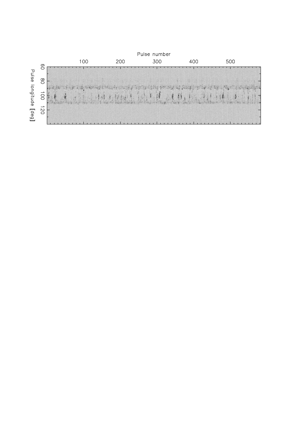
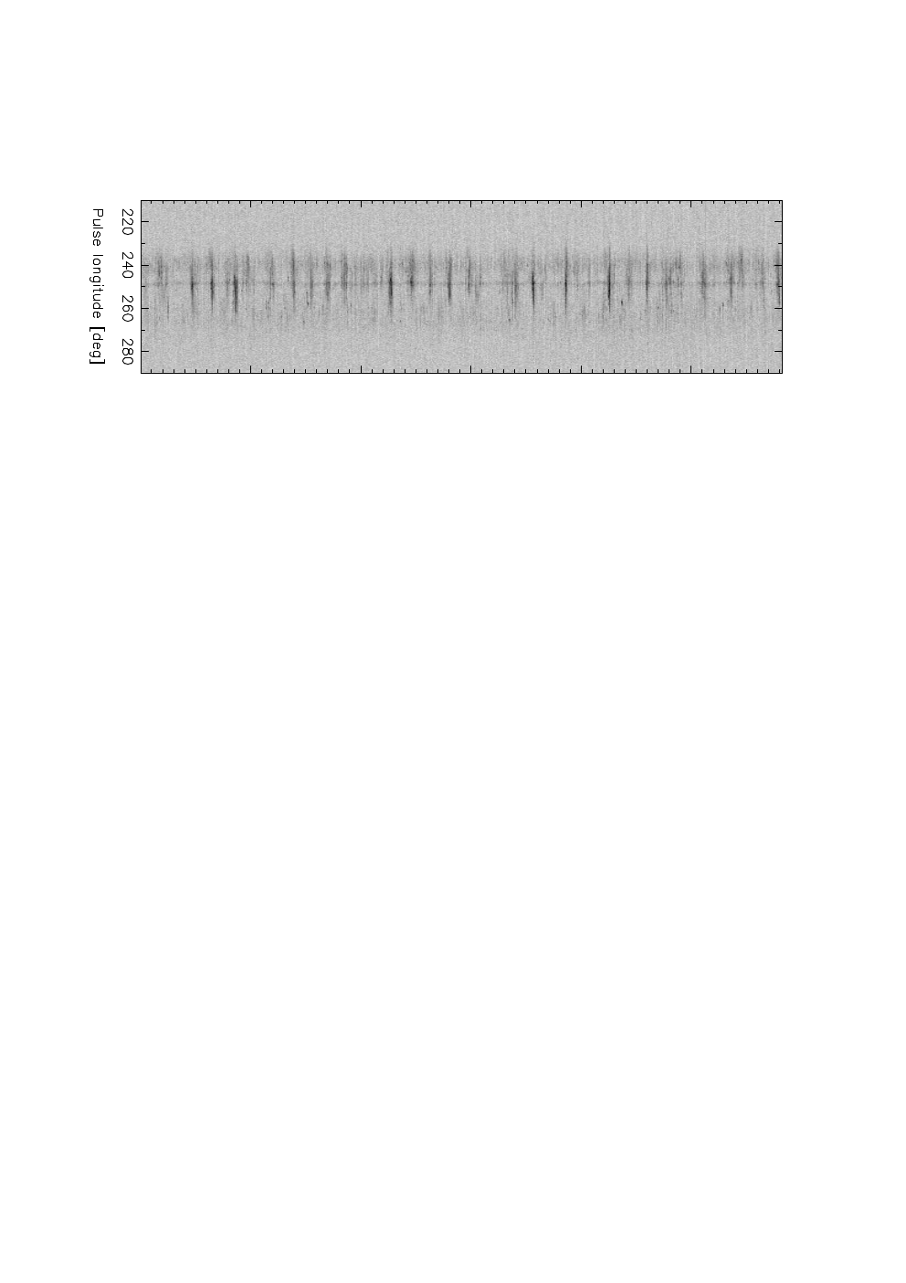
Before embarking on a detailed analysis of the statistical properties of the emission of PSR B1055–52, it is good to first get a basic understanding of its behaviour by inspecting some of its individual pulses by eye. The pulse-stacks of the MP and IP of PSR B1055–52 are plotted in Fig. 2 with the pulse longitude scale aligned with that of Fig. 1 by placing the profile peak at pulse longitude $90^{\circ}$. As one can see, the pulse intensities are highly variable from pulse to pulse. The most obvious modulation pattern is the roughly periodic brightening which happens on a timescale of $\sim 20P$. This modulation is especially visible in the IP and the third component of the MP (at $\sim 100^{\circ}$ pulse longitude).

Periodicities in pulse intensity are a common phenomenon in radio pulsars (e.g. Weltevrede et al., 2006; Weltevrede et al., 2007), often associated with drifting subpulses (Drake & Craft, 1968), although in the case of PSR B1055–52 the periodicity arises from intensity modulations rather than phase modulations. We will show in Sect. 3.7 that there exists a stable phase delay between the modulation patterns observed in the MP and IP, a feature which in fact is detectable by eye in Fig. 2.

The various components of the pulse profile have completely different characteristics in their single pulse behaviour. It is particularly striking that the pulses of the MP have a very different appearance to those of the IP. The pulses of the MP show much sharper structures and can have widths much smaller than the profile component widths. In contrast the individual pulses of the IP are much more extended or smeared out in pulse longitude. The pulses of the MP, especially those of component II (pulse longitude $\sim 90^{\circ}$), can be characterised as very spiky, i.e. the pulse-stack at the location of component II is dotted with narrow spikes of emission with high peak fluxes thereby resembling the emission observed, for instance, in PSR B0656+14 (Weltevrede et al., 2006). Furthermore, it appears that not every MP component shares the $20P$ modulation as clearly as some of the others.

Also within the IP the individual components have differing single-pulse characteristics. Although component VI (pulse longitude $\sim 248^{\circ}$) participates in the modulation cycle, it never fades as much as the other IP components, thereby forming a vertical band in the pulse-stack. In addition, component V (pulse longitude $\sim 240^{\circ}$) and VII (pulse longitude $\sim 260^{\circ}$) while also subject to modulation, do not completely disappear. The middle component (VI) appears to form some sort of boundary in the sense that sometimes the leading side of the IP profile participates much more strongly in the modulation cycle compared to the trailing side (e.g. around pulse 96 and 245) and sometimes this appears to be reversed (e.g. around pulse 85 and 355). Nevertheless in many cases both components clearly show the same cycle. The duty cycle of the $\sim 20P$ modulation pattern is relatively small in both the MP and IP with the pattern being bright for only a few pulses.

The time-averaged properties of the periodic subpulse modulation can be studied in more detail by calculating fluctuation spectra. We will follow the methods developed by Edwards & Stappers (2002) and for more details about the analysis we also refer to Weltevrede et al. (2006). The first type of fluctuation spectrum computed is the longitude-resolved fluctuation spectrum (LRFS; Backer 1970). This fluctuation spectrum is obtained by separating the pulse-stack into blocks of 256 pulses long. By calculating Fourier transforms along constant pulse longitude columns in the pulse-stack one gets information about the periodicities present for each pulse longitude bin. By averaging the square of the spectra obtained for the consecutive blocks of data the LRFS is obtained. These spectra are shown in the middle panels of Fig. 3.

The LRFS confirms and clarifies the features noted by eye in the pulse-stack. The LRFS of the IP clearly shows the $\sim 20P$ periodicity, which corresponds to $\sim 0.05$ cycles per period (cpp). The same periodicity is visible in the LRFS of the MP (especially in the trailing half of component II at $90^{\circ}$ and component III at $100^{\circ}$), although there is much more additional modulation power at different frequencies (or timescales) compared to the IP. This is consistent with the $\sim 20P$ periodicity visible most clearly in the pulse-stack of the IP. As can be seen in the side panel of the LRFS of the MP, the spectral power appears to be a combination of a white-noise like plateau combined with a peak corresponding to the $\sim 20P$ periodicity and a red-noise like spectrum corresponding to timescales larger than $\sim 5P$ (corresponding to frequencies smaller than $\sim 0.02$ cpp). The different profile components show different mixtures of these spectral behaviours.

The two dimensional fluctuation spectrum (2DFS; Edwards & Stappers 2002) is a different type of fluctuation spectrum that can reveal additional information about periodic subpulse modulation. The vertical frequency axis is very similar to the case of the LRFS, which can be expressed as $P/P_{3}$, where $P_{3}$ corresponds to the $20P$ periodicity visible in the pulse-stack. The horizontal axis of the 2DFS denotes a frequency as well, which can be expressed as $P/P_{2}$, where $P_{2}$ corresponds to the horizontal separation of the subpulses. If the power were concentrated at positive values of $P_{2}$ it would indicate that subpulses tend to shift (or drift) to later pulse longitudes in successive pulses.

The IP shows the same $P_{3}=21\pm 2P$ periodicity (for a discussion about error bars on fluctuation frequencies, see Weltevrede et al. 2006) and its 2DFS is perfectly symmetric about the vertical axis. This indicates that subpulses in successive pulses do not drift on average to later or earlier pulse longitudes, which is consistent with the fact that the intensity bands in the pulse-stack of the IP appears to be horizontal. The 2DFS of the MP has a much more complex shape. As expected from inspection of the LRFS, the 2DFS of the MP also shows power corresponding to a wider range of periodicities. There is horizontal structure visible in the 2DFS with power concentrated on frequencies corresponding to the component separations within the MP. The asymmetry of the 2DFS about the vertical axis indicates that the appearance of subpulses in the different components is correlated, although the correlation is complex in nature. The possible pulse longitude drift of subpulses participating in the $P_{3}\simeq 20P$ cycle will be explored in more detail in Section 3.7.

The peaks in the LRFS and 2DFS caused by the $P_{3}\simeq 20P$ cycle is broad, hence the periodicity does not appear to be particularly stable. Although the first signs are not promising, we pursued the possibility that a very precise and stable clock is responsible for the observed periodicity, although modulated by a noise-like process. The presence of such a stable signal would have important consequences, for instance when the periodicity is linked to a possible fallback debris disks (Cordes & Shannon, 2008).

The possible presence of a stable periodicity among other time-varying signals can be tested by making use of the sliding 2DFS (S2DFS; Serylak et al. 2009). The S2DFS is a time-resolved version of the 2DFS and is therefore ideal to analyse the time-dependence of the $P_{3}\simeq 20P$ cycle. The S2DFS is calculated by computing the 2DFS for blocks of 256 pulses with the start of the block shifting with one pulse at the time. In other words, the first 2DFS is computed from pulses $1-256$, the second for pulses $2-257$, etc. The two dimensional spectra are collapsed over the $P_{2}$ axis, giving rise to a one dimensional spectrum for each block. By stacking the resulting spectra for the successive blocks of data one obtains the S2DFS (see Fig. 4). The spectra obtained for these “block numbers” are not independent of each other, as the time resolution is determined by the size of the sliding window of 256 pulses. The S2DFS shows a constantly changing frequency of the modulation pattern and no fixed periodicity is present among the other time-variable fluctuations. The second conclusion is that the timescale of the time-variability of the modulation pattern is short, i.e. a few hundred pulses or less.

Secondly we tested the hypothesis that the observed $P_{3}\simeq 20P$ cycle is a very stable periodicity affected by a large phase-noise. In other words, could it be possible that the bright intensity bands in the pulse-stack appear often a few pulses earlier or later then what would be predicted by an otherwise strictly periodic cycle? In some ways this is analogous to what is assumed for pulsar timing experiments, where the pulse arrival times are compared to a timing model containing well defined periodicities, giving rise to timing residuals with relatively small amplitude. By making use of the timing software developed by Weltevrede et al. (2011) we tried to model the measured pulse numbers for which we observe a bright intensity band in the IP with a timing model being a fixed frequency. This frequency was initially set to the frequency of the peak in the LRFS obtained for the same stretch of data of a few hundred pulses long which was used to measure the pulse numbers corresponding to the appearance of the intensity bands. It turns out to be impossible to get phase connection of the measured arrival times of the intensity bands, even after changing the frequency in the timing model. This confirms the suspicion that the periodicity of the modulation pattern is unstable, rather being a fixed value modulated by phase noise with an amplitude less than $20P$.

The upper panels of Fig. 3 show, besides the pulse profile (grey curve), the longitude resolved modulation index of the MP and IP. The modulation index is a normalised measure of the variability of the pulse intensities at a given pulse longitude and is computed from the LRFS (see e.g. Edwards & Stappers 2003; Weltevrede et al. 2006). The error bars on the modulation index was derived by bootstrapping the data (pulse-stack). For each iteration in the bootstrap method an equivalent pulse-stack was generated by adding random noise samples with an root-mean-square (rms) equal to that measured in the off-pulse region. The standard deviation of the distribution of modulation indices obtained in this way is set to be the (1-$\sigma$) error bar. Simulations with artificial pulse-stacks indicate that the error bars derived in this way are more reliable than the analytically estimated error bars as computed for instance by Edwards & Stappers (2003) and Weltevrede et al. (2006).

Typically one measures modulation indices of around $0.5$ (at observing frequencies around 1400 MHz; e.g. Weltevrede et al. 2006) at the centre of components with the modulation index flaring up at the component edges. A similar flaring up at the profile edges is seen for this pulsar. The most variable pulse intensities (i.e. highest modulation index) are seen between components II and III of the MP. The value of the modulation index in this region of the MP is as large as that observed for PSR B0656+14 at a frequency of 327 MHz (Weltevrede et al., 2006). However one cannot direct compare these values because the high modulation index of PSR B1055–52 is observed between profile components, while that of PSR B0656+14 is observed at the profile centre (which is what makes the high modulation index of PSR B0656+14 unusual). The modulation index derived from the BPSR data is similar, suggesting that the high modulation index is not caused by the baseline artifact.

The modulation index profile of the IP is on average lower than that of the MP. This is not surprising given the much more spiky appearance of the pulse-stack of the MP. The modulation index profile shows a dip at the location of component VI, which is caused by the presence of steady emission in that component (as is seen as the vertical band in the pulse-stack in Fig. 2).

Biggs (1990) reports that the pulse profile of PSR B1055–52 is variable at relatively long timescales in the sense that the peak amplitudes of the different components fluctuate when integrations of $2000P$ are taken. In order to quantify this effect we averaged pulses in blocks of 2000 pulses. Using the methods outlined in the previous subsection we calculated the longitude resolved modulation index and standard deviation (after rebinning the data to 200 pulse longitude bins). As can be seen in Fig. 5, the highest variability (the open circles indicating the standard deviation of the intensities at a given pulse longitude) is observed in component II (pulse longitude $\sim 90^{\circ}$). However, after normalisation with respect to the average intensity observed at these longitudes (i.e. the modulation index; the points with error bars) one can see this variability is not exceptional compared to other components in the MP. The emission of the IP is more stable resulting in a low modulation index for the profile variability which is comparable to that observed in component IV in the MP (pulse longiture $\sim 110^{\circ}$). This is consistent with the more spiky nature of the emission observed for the MP, hence longer stabilisation timescales can be expected as is observed for PSR B0656+14 (Weltevrede et al., 2006).

Unlike Biggs (1990), we find that component II has the largest amplitude throughout the observation, while Biggs (1990) observed component III to have in general the largest amplitude⁴⁴ 4 In the component name convention of Biggs (1990) this corresponds to component I and II rather than components II and III.. We have found no exception to this rule in 67 observations of this pulsar between 2007 and 2011 for the Fermi timing program at Parkes (Weltevrede et al., 2010). It must be noted that our observing wavelength (around $20$ cm) is different from that in Biggs (1990) (around $50$ cm), but the profile evolution between these frequencies is not very strong (see e.g. Fig. 2 in Weltevrede & Wright 2009). We attribute these differences in the profile to instrumental effects in the observations of Biggs (1990), which had a much lower time resolution. Later Parkes radio observations as shown by for instance Wu et al. (1991); van Ommen et al. (1997); Thompson et al. (1999) are consistent with the observations presented in this paper.

The fluctuation spectra have shown us in some detail about periodicities in the pulse intensity. The modulation index tells us, in a very limited way, how variable the pulse intensities are. More detailed information about the intensity variations can be obtained by making a pulse energy distribution. The pulse energy distribution is calculated by integrating the intensities as recorded in the pulse-stack over a pulse longitude range. This has been done for the full pulse longitude range of the MP and IP separately, which gives a pulse energy $E_{i}$ for each stellar rotation $i$. Given that the observations were not flux calibrated, only the values $E_{i}$ relative to each other are meaningful. We therefore choose to normalise the pulse energies $E_{i}$ by $\left<E_{\mathrm{MP}}\right>$, the average pulse energy measured for the MP. Closer inspection of the data reveals that the flux of PSR B1055–52 is not constant throughout the observation because of interstellar scintillation. The pulsar is weak at the start and end of the observation, but has a nearly constant flux for 35 minutes. The energy distributions shown in Fig. 6 are therefore based on these 35 minutes, which much more accurately reflect the intrinsic pulse energy distribution of the source. The off-pulse energy distributions (noise distributions) are shown as well in order to quantify the uncertainty in the pulse energy measurements (dashed grey distributions). The off-pulse energy distribution is calculated by integrating the off-pulse region over a pulse longitude window with equal width compared to the on-pulse window.

Using the methods explained in Weltevrede et al. (2006) we have fit the shape of the energy distribution of the IP by a log-normal distribution convolved with the observed noise distribution. The parameters of the lognormal distribution

we fit for are found to be $\mu=-0.13$ and $\sigma=0.51$. This fit matches the observed energy distribution of the IP very well (see centre panel of Fig. 6).

The fit for the IP energy distribution is reproduced in the left panel of Fig. 6 (without any scaling). As one can see the shapes of the energy distribution observed for the MP and IP (centre panel of Fig. 6) are very similar. This close resemblance is surprising given the completely different characteristics of the pulses as can be seen in the pulse-stack (see Fig. 2) and given the conclusion in Section 3.2 that the fluctuation spectra of especially the MP can be described by a mixture of different emission types. The resemblance of the MP and IP energy distribution is confirmed in other (shorter) observations.

There are small differences in the shape of the energy distribution of the MP and IP. The IP shows a tail beyond $E_{i}\,\raisebox{-1.29167pt}{\mbox{$\stackrel{{\scriptstyle>}}{{{}_{\sim}}}\,$}}4\left<E_{\mathrm{MP}}\right>$ which is not present in the MP and a slight excess of MP pulses with energies in the range $2\left<E_{\mathrm{MP}}\right>\,\raisebox{-1.29167pt}{\mbox{$\stackrel{{\scriptstyle<}}{{{}_{\sim}}}\,$}}E_{i}\,\raisebox{-1.29167pt}{\mbox{$\stackrel{{\scriptstyle<}}{{{}_{\sim}}}\,$}}4\left<E_{\mathrm{MP}}\right>$. In addition the energy distribution of the MP is skewed to slightly lower energies at the low-energy part compared to that of the IP. Closer inspection reveals that the energy distributions of most of the individual components are very similar to the shape of the overall energy distribution of the MP and IP. The exception is component III, which shows a clear break in its pulse energy distribution (see right panel of Fig. 6) and component I, which is too weak to accurately determine its pulse energy distribution. The different shape of the pulse energy distribution of component III is therefore responsible for the slight difference in the overall energy distribution of the MP and IP.

Motivated by the similarity between the pulse energy distribution of the MP and IP, we investigated if the pulse energies of the MP and IP are correlated at timescales slightly longer than the modulation cycle. Following a similar procedure employed by Weltevrede et al. (2007) for PSR B1702–19, we started by averaging blocks of 20 pulses. This ensured that the modulation pattern is no longer present in the signal, which was confirmed by calculating the LRFS. MP and IP energies were calculated for each block by integrating over the full pulse longitude range over which emission was detectable in the pulse profile. Finally, by cross correlating the MP and IP sequence of energies it was possible to investigate if the power output of the MP and IP are related. However, there was very little evidence for correlation between the MP and IP power output on timescales larger than the modulation cycle, apart from long-term correlations caused by the fact that both the MP and IP are affected simultaneously by interstellar scintillation.

The fact that the MP and IP both show a similar periodic modulation pattern is already a remarkable result in itself. We will explore this similarity further by determining any phase relations of the $\sim 20P$ modulation pattern observed in the different profile components. The technique used to obtain this phase relation as function of pulse longitude is based on fluctuation spectra. Firstly the (complex) LRFS was calculated for 128 pulses long blocks of data. Instead of calculating the square of the complex numbers in the spectrum, as is done to obtain the LRFS as shown in Fig. 3, the phases were calculated. By selecting the spectral bin that showed the $\sim 20P$ modulation pattern strongest (which was at 0.046875 cpp), the so-called subpulse phase as function of pulse longitude was obtained (Edwards & Stappers, 2002). The complex numbers obtained for the different blocks of data are added coherently using an iterative scheme designed to maximize the correlation between the phase profiles of the different blocks in the on-pulse region. This is achieved by allowing an arbitrary phase offset, which is constant with pulse longitude, between the different blocks of data. The coherent addition gives rise to the complex subpulse modulation envelope, with the complex phase corresponding to the subpulse phase. Error bars on the subpulse phase were calculated by applying a bootstrap scheme similar to the one employed in Section 3.4 for the modulation index.

The result of the calculation is shown in the lower panels of Fig. 7. The actual value of the subpulse phase is not an intrinsic property of the pulsar, but phase differences between different pulse longitudes are. We have therefore arbitrarily chosen the subpulse phase to be zero at the centre of the IP. The upper panels of Fig. 7 show, in addition to the pulse profile, the amplitude of the subpulse modulation corresponding to the amplitude of the complex modulation envelope⁵⁵ 5 The normalisation of the subpulse amplitude profile is such that for a pure sinusoidal signal with a frequency equal to the centre of a frequency bin in the complex LRFS the subpulse amplitude profile matches the pulse profile with its peak amplitude normalised to 1. (see Edwards & Stappers 2002; Edwards et al. 2003). Note that this amplitude depends on the coherence of the modulation pattern (i.e. the stability of the longitude dependence of the subpulse phase as function of pulse longitude). The results obtained are identical in the first and second half of the data and for the data which was not corrected for the baseline artifact. In addition the BPSR data gave identical results, although the pulsar was much weaker during that observation. Hence we are confident that the features of Fig. 7, both at the MP and IP, are stable and intrinsic properties of the star rather than instrumental effects.

The subpulse phase relation with pulse longitude reveals a high degree of complexity, especially for the MP. Concentrating on the IP first, we see that the subpulse phase is roughly independent of pulse longitude. This means that that the modulation cycle seen in different pulse longitude bins of the IP are in phase, hence the intensity bands seen in the pulse-stack are to a good approximation horizontal (at least on average). This lack of phase drift makes it unclear if the physical mechanism responsible for the modulation pattern is the same as is operating in pulsars with drifting subpulses. At the outer edges of the IP profile the modulation pattern appears to be slightly out of phase such that the subpulse phase decreases away from the central parts of the profile. This indicates that the modulation pattern is slightly lagging at the centre of the IP. The central peak of the IP at pulse longitude $\sim 248^{\circ}$ does reveal a slight deviation in subpulse phase as well.

In the MP, at the longitudes where the $20P$ modulation is strongest (pulse longitudes $88^{\circ}-105^{\circ}$), the subpulse phase appears to be roughly in phase as well, although revealing a weak decline corresponding to a gradual drift from trailing to leading components. The subpulse phase offset between the IP and the central parts of the MP is about $40^{\circ}$, which corresponds to a delay of $\sim 2.5P$ such that the pattern in the MP is late compared to that of the IP. It must be noted that if the modulation patterns in two pulse longitude bins are intrinsically in phase (in the pulsar frame), they will be observed out of phase because later pulse longitudes are observed later in time, allowing the pattern to change during the rotation of the star. The slope in subpulse phase expected to be observed if the modulation is intrinsically in phase is indicated by the almost horizontal baseline in Fig. 7 continued through from the MP to the IP. We can conclude that the $\sim 20P$ modulation cycle of the IP is intrinsically out of phase with the modulation of the MP at any longitude and that the observed phase delay of the modulation patterns corresponds to an intrinsic delay of $\sim 3P$. As will be discussed in Section 4, this delay corresponds to an extremely long light travel distance which is much larger than the light-cylinder radius, thereby challenging existing theories for pulsar emission to explain this.

The phase delay between the MP and the IP can be demonstrated in a different way by correlating the measured pulse energies for successive pulses in the MP and IP. The cross correlation function, using the regions in the MP and IP where the modulation is strongest, is shown in Fig. 8. The $\sim 20P$ modulation cycle is clearly visible in the correlation function, showing that the modulation patterns in the MP and IP are phase-locked independent of any jitter in the periodicity of the pattern. The phase offset in the patterns gives rise to an offset of the peak of the correlation function from zero lag. The shift can be determined by comparing the offset between the cross correlation curve and the time reversed correlation function, which is set to $5P$ in the figure. This offset is equal to twice the offset of the symmetric curve from zero lag and therefore confirms the lag of $\sim 2.5P$ of the pattern observed in the MP compared to that in the IP.

The behaviour described so far is accompanied by a number of strong diversions. The modulation pattern in the trailing peak of the MP (at pulse longitude $110^{\circ}$) appears to be out of phase with that in the more central regions by $\sim 80^{\circ}$, corresponding to a delay of almost $5P$. More subtle is the change in subpulse phase in component II at the location of the strongest presence of the $\sim 20P$ modulation (pulse longitude $\sim 90^{\circ}$). Although the subpulse phase is approximately longitude stationary in that pulse longitude range, it decreases towards pulse longitude $90^{\circ}$, indicating that the pattern is observed early at the pulse longitudes where the modulation is strongest. Close examination of the MP profile in Fig. 7 reveals that component II is in fact composed of two components which overlap. The trailing half of component II shows the $20P$ modulation strongest, suggesting that only one of the two overlapping components strongly participates in the modulation cycle.

At the pulse longitudes where the amplitude of the $\sim 20P$ modulation pattern is weakest the subpulse phase has the most complex pulse longitude dependence. In the first half of component II (pulse longitude $\sim 86^{\circ}$) a rapid swing in subpulse phase occurs which cover almost a complete modulation cycle of $\sim 20P$ (corresponding to $360^{\circ}$ in subpulse phase). Similarly between components III and IV (around pulse longitude $107^{\circ}$) the modulation power disappears accompanied by a steep negative slope in the subpulse phase gradient. We note, however, that the power affected by this feature is very weak compared with the total power in the modulation pattern.

The main conclusion of the subpulse phase analysis is that the regions where the $\sim 20P$ modulation pattern is strongest a firm phase-locking is present between the MP and IP. We note that the delay accompanied by this phase-locking is found to be identical in completely different observations recorded at different dates. This implies that the locking is sustained over periods much greater than the duration of a single observation and is likely to be a permanent feature of the pulsar.

The essentially geometric results of Paper I, and those presented hitherto in this paper, make no physical assumptions other than that we are observing a rotating dipole emitting polarized radiation parallel to its field lines. To develop a physical understanding, we need to explain (1) the origin of the dominant $\sim 20P$ modulation cycle, (2) why there is a considerable phase-locked delay between the IP emission and that at the MP and (3) why this pulsar emits radiation on field lines which are normally deemed to be closed.

References

- Abdo et al. (2010) Abdo A. A., et al. 2010, ApJ, 720, 26
- Backer (1970) Backer D. C., 1970, Nature, 227, 692
- Backus et al. (2010) Backus I., Mitra D., Rankin J. M., 2010, MNRAS, 404, 30
- Becker & Trümper (1997) Becker W., Trümper J., 1997, A&A, 326, 682
- Biggs (1990) Biggs J. D., 1990, MNRAS, 246, 341
- Burke-Spolaor et al. (2012) Burke-Spolaor S., Johnston S., Bailes M., Bates S. D., Bhat N. D. R., Burgay M., Champion D. J., D’Amico N., Keith M. J., Kramer M., Levin L., Possenti S. M. A., Stappers B., van Straten W., 2012, submitted to MNRAS (arXiv:1203.6068)
- Clemens & Rosen (2004) Clemens J. C., Rosen R., 2004, ApJ, 609, 340
- Cordes & Shannon (2008) Cordes J. M., Shannon R. M., 2008, ApJ, 682, 1152
- Drake & Craft (1968) Drake F. D., Craft H. D., 1968, Nature, 220, 231
- Dyks (2008) Dyks J., 2008, MNRAS, 391, 859
- Dyks et al. (2010) Dyks J., Wright G. A. E., Demorest P., 2010, MNRAS, 405, 509
- Edwards & Stappers (2002) Edwards R. T., Stappers B. W., 2002, A&A, 393, 733
- Edwards & Stappers (2003) Edwards R. T., Stappers B. W., 2003, A&A, 407, 273
- Edwards et al. (2003) Edwards R. T., Stappers B. W., van Leeuwen A. G. J., 2003, A&A, 402, 321
- Everett & Weisberg (2001) Everett J. E., Weisberg J. M., 2001, ApJ, 553, 341
- Fowler & Wright (1982) Fowler L. A., Wright G. A. E., 1982, A&A, 109, 279
- Fowler et al. (1981) Fowler L. A., Wright G. A. E., Morris D., 1981, A&A, 93, 54
- Gil et al. (1994) Gil J. A., Jessner A., Kijak J., Kramer M., Malofeev V., Malov I., Seiradakis J. H., Sieber W., Wielebinski R., 1994, A&A, 282, 45
- Gil & Sendyk (2000) Gil J. A., Sendyk M., 2000, ApJ, 541, 351
- Hankins & Eilek (2007) Hankins T. H., Eilek J. A., 2007, ApJ, 670, 693
- Keith et al. (2010) Keith M. J., Jameson A., van Straten W., Bailes M., Johnston S., Kramer M., Possenti A., Bates S. D., Bhat N. D. R., Burgay M., Burke-Spolaor S., D’Amico N., Levin L., McMahon P. L., Milia S., Stappers B. W., 2010, MNRAS, 409, 619
- Keith et al. (2010) Keith M. J., Johnston S., Weltevrede P., Kramer M., 2010, MNRAS, 402, 745
- Luo & Melrose (2007) Luo Q., Melrose D., 2007, MNRAS, 378, 1481
- Lyne et al. (2010) Lyne A., Hobbs G., Kramer M., Stairs I., Stappers B., 2010, Science, 329, 408
- Melrose & Yuen (2011) Melrose D. B., Yuen R., 2011, ArXiv e-prints (astro-ph/1107.0100)
- Michel & Dessler (1981) Michel F. C., Dessler A. J., 1981, ApJ, 251, 654
- Rankin (1986) Rankin J. M., 1986, ApJ, 301, 901
- Radhakrishnan & Cooke (1969) Radhakrishnan V., Cooke D. J., 1969, ApJ, 3, 225
- Romani & Watters (2010) Romani R. W., Watters K. P., 2010, ApJ, 714, 810
- Ruderman & Sutherland (1975) Ruderman M. A., Sutherland P. G., 1975, ApJ, 196, 51
- Serylak et al. (2009) Serylak M., Stappers B. W., Weltevrede P., 2009, A&A, 506, 865
- Thompson et al. (1999) Thompson D. J., Bailes M., Bertsch D. L., Cordes J., D’Amico N., Esposito J. A., Finley J., Hartman R. C., Hermsen W., Kanbach G., Kaspi V. M., Kniffen D. A., Kuiper L., Lin Y. C., Manchester R., Matz S. M., Mayer-Hasselwander H. A., Michelson P. F., et al. 1999, ApJ, 516, 297
- Thompson et al. (1999) Thompson D. J., et al. 1999, ApJ, 516, 297
- Tsygan (1977) Tsygan A. I., 1977, Soviet Astronomy Letters, 3, 289
- van Ommen et al. (1997) van Ommen T. D., D’Alesssandro F. D., Hamilton P. A., McCulloch P. M., 1997, MNRAS, 287, 307
- Wang et al. (2006) Wang H. G., Qiao G. J., Xu R. X., Liu Y., 2006, MNRAS, 366, 945
- Weltevrede et al. (2006) Weltevrede P., Edwards R. T., Stappers B. W., 2006, A&A, 445, 243
- Weltevrede & Johnston (2008) Weltevrede P., Johnston S., 2008, MNRAS, 387, 1755
- Weltevrede et al. (2011) Weltevrede P., Johnston S., Espinoza C. M., 2011, MNRAS, 411, 1917
- Weltevrede et al. (2010) Weltevrede P., Johnston S., Manchester R. N., Bhat R., Burgay M., Champion D., Hobbs G. B., Kızıltan B., Keith M., Possenti A., Reynolds J. E., Watters K., 2010, PASA, 27, 64
- Weltevrede et al. (2007) Weltevrede P., Stappers B. W., Edwards R. T., 2007, A&A, 469, 607
- Weltevrede & Wright (2009) Weltevrede P., Wright G., 2009, MNRAS, 395, 2117
- Weltevrede et al. (2007) Weltevrede P., Wright G. A. E., Stappers B. W., 2007, A&A, 467, 1163
- Weltevrede et al. (2006) Weltevrede P., Wright G. A. E., Stappers B. W., Rankin J. M., 2006, A&A, 458, 269
- Wright (1979) Wright G. A. E., 1979, Nature, 280, 40
- Wright (2003) Wright G. A. E., 2003, MNRAS, 344, 1041
- Wu et al. (1991) Wu X.-J., Manchester R. N., Lyne A. G., 1991, Acta Astrophysica Sinica, 11, 227