Throughput Optimal Policies for Energy Harvesting Wireless Transmitters with Non-Ideal Circuit Power
Abstract
Characterizing the fundamental tradeoffs for maximizing energy efficiency (EE) versus spectrum efficiency (SE) is a key problem in wireless communication. In this paper, we address this problem for a point-to-point additive white Gaussian noise (AWGN) channel with the transmitter powered solely via energy harvesting from the environment. In addition, we assume a practical on-off transmitter model with non-ideal circuit power, i.e., when the transmitter is on, its consumed power is the sum of the transmit power and a constant circuit power. Under this setup, we study the optimal transmit power allocation to maximize the average throughput over a finite horizon, subject to the time-varying energy constraint and the non-ideal circuit power consumption. First, we consider the off-line optimization under the assumption that the energy arrival time and amount are a priori known at the transmitter. Although this problem is non-convex due to the non-ideal circuit power, we show an efficient optimal solution that in general corresponds to a two-phase transmission: the first phase with an EE-maximizing on-off power allocation, and the second phase with a SE-maximizing power allocation that is non-decreasing over time, thus revealing an interesting result that both the EE and SE optimizations are unified in an energy harvesting communication system. We then extend the optimal off-line algorithm to the case with multiple parallel AWGN channels, based on the principle of nested optimization. Finally, inspired by the off-line optimal solution, we propose a new online algorithm under the practical setup with only the past and present energy state information (ESI) known at the transmitter.
Index Terms:
Energy harvesting, power control, energy efficiency, spectrum efficiency, circuit power.I Introduction
Green or energy efficient wireless communication has recently drawn significant attention due to the growing concerns about the operator’s cost as well as the global environmental cost of using fossil fuel based energy to power cellular infrastructures [1, 2, 3]. To achieve the optimal energy usage efficiency for cellular networks, various innovative “green” techniques across different layers of communication protocol stacks have been proposed [4, 5]. Among others, how to maximize the bits-per-Joule energy efficiency (EE) for the point-to-point wireless link has received a great deal of interest recently [6, 7, 8].

Besides maximizing EE, another key design objective in wireless communication is to maximize the spectrum efficiency (SE) or the number of transmitted bits-per-second-per-Hz (bps/Hz), due to the explosive growth of wireless devices and applications that require high data rates. In order to design wireless communication systems both energy and spectrum efficiently, the fundamental EE-SE relationship needs to be examined carefully. For the simple additive white Gaussian noise (AWGN) channel with bandwidth and noise power spectral density , by applying the Shannon’s capacity formula, the SE and EE are expressed as and , respectively, with denoting the transmit power. It thus follows that the optimal EE-SE tradeoff is characterized by , where is a monotonically decreasing function of , as shown in the left sub-figure of Fig. 1. In this case, any SE increment will inevitably result in a decrement in EE. However, in practical wireless transmitters, besides the direct transmit power , there also exists non-ideal circuit power consumed when , which accounts for the power consumptions at e.g. the AC/DC converter and the analog radio frequency (RF) amplifier, and amounts to a significant part of the total consumed power at the transmitter. Moreover, when there is no data transmission, i.e., , the transmitter can turn into a micro-sleep mode [9], by switching off the power amplifier to reduce the circuit power consumption. For the ease of description, in this paper the transmitter status with and are referred to as the on and off modes, respectively. Denote the non-ideal circuit power during an “on” mode as in Watt, the efficiency of the RF chain as , and the power consumed during an “off” mode as in Watt. A practical power consumption model for the wireless transmitter is given by [10]
where denotes the total power consumed at the transmitter. In practice, is generally much smaller as compared to and thus can be ignored for simplicity [5, 7, 8]. In this paper, we assume . Therefore, in (I) without loss of generality we can further assume since is only a scaling constant.11 1 Note that the results of this paper can be readily extended to the case with by appropriately scaling the obtained solutions. With the above simplifications, the EE can be re-expressed as for and the resulting new EE-SE tradeoff is shown in the right sub-figure of Fig. 1 for a given , from which it is observed that the non-ideal circuit power drastically changes the behavior of the EE-SE tradeoff as compared to the ideal case of .
Recently, a new design paradigm for achieving green wireless communication has drawn a great deal of attention, in which wireless terminals are powered primarily or even solely by harvesting the energy from environmental sources such as solar and wind, thereby reducing substantially the energy cost in traditional wireless systems [4, 11]. With the embedded energy harvesting device and rechargeable battery, wireless transmitters can replenish energy from the environment without the need of replacing battery or drawing power from the main grid. Thus, communication utilizing energy harvesting nodes can promisingly achieve a jointly spectrum and energy efficiency maximization goal. However, there are new challenges in designing energy harvesting powered wireless communication, which are not present in traditional systems. For example, the intermittent nature of most practical energy harvesting sources causes random power availability at the transmitter, due to which a new type of transmitter-side power constraint, namely energy harvesting constraint, is imposed, i.e., the energy accumulatively consumed up to any time cannot exceed that accumulatively harvested. As a result, existing EE-SE tradeoffs (cf. Fig. 1) revealed for conventional wireless systems assuming a given constant power supply are not directly applicable to an energy harvesting system, with or without the non-ideal circuit power. It is worth noting that some prior work in the literature has investigated the throughput-optimal power control policies for the energy harvesting wireless transmitter assuming an ideal circuit-power model (i.e., , and in (I)), in which useful structural properties of the optimal solution were obtained (see e.g. [12, 13, 14] and references therein). However, there is very limited work on studying the effects of the non-ideal circuit power with on the throughput-optimal power allocation for energy harvesting communication systems. To our best knowledge, only [15] has proposed a calculus-based approach to address this problem; however, it does not reveal the structure of the optimal solution. Motivated by the known result that the non-ideal circuit power modifies the EE-SE tradeoff considerably in the conventional case with constant power supply as shown in Fig. 1, we expect that it should also play an important role in the EE-SE tradeoff characterization under the new setup with random power supply due to energy harvesting, which motivates our work.
In this paper, we study the throughput maximization problem for a point-to-point AWGN channel with an energy harvesting powered transmitter over a finite horizon. For the purpose of exposition, we assume that the receiver has a constant power supply (e.g. battery). We also assume that at the transmitter, the renewable energy arrives at a discrete set of time instants with variable energy amount. Under this setup, we investigate the effects of the non-ideal circuit power with on the throughput-optimal power allocation as well as the resulting new EE-SE tradeoff. The main contributions of this paper are summarized as follows.
- •
First, we consider the off-line optimization under the assumption that the energy arrival time and amount for harvesting are a priori known at the transmitter. We show that the optimal power allocation to maximize the average throughput under this setup is a non-convex optimization problem, due to the non-ideal circuit power. Nevertheless, we derive an efficient optimal solution for this problem, which is shown to correspond to a novel two-phase transmission structure: the first phase with an EE-maximizing on-off power allocation, and the second phase with a SE-maximizing power allocation that is non-decreasing over time. Thus, we reveal an interesting result that both the EE and SE optimizations are unified in an energy harvesting powered wireless system.
- •
We then extend the optimal off-line policy for the single-channel case to the general case with multiple parallel AWGN channels, subject to a total energy harvesting power constraint. Using tools from nested optimization, we transform this problem with multi-dimensional (vector) power optimization to an equivalent one with only one-dimensional (scalar) power optimization, which can then be efficiently solved by the algorithm derived for the single-channel case.
- •
Furthermore, inspired by the off-line optimal solution, we propose a heuristic online algorithm under the practical setup where only the causal (past and present) energy state information (ESI) for harvesting is assumed to be known at the transmitter. It is shown by simulations that the proposed online algorithm achieves a small performance gap from the throughput upper bound by the optimal off-line solution, and also outperforms other heuristically designed online algorithms.
The rest of this paper is organized as follows. Section II introduces the system model and presents the problem formulation. Section III derives the optimal off-line power allocation policy for the single-channel case. Section IV extends the result to the multi-channel case based on the nested optimization. Section V presents the proposed online algorithm and Section VI evaluates its throughput performance by simulations. Finally, Section VII concludes the paper.
II System Model and Problem Formulation
In this paper, we consider the point-to-point transmission over an AWGN channel with constant channel and coherent detection at the receiver. The transmitter is assumed to replenish energy from an energy harvesting device that collects energy over time from a renewable source (e.g. solar or wind). We consider the block-based energy scheduling with each block spanning over seconds (secs). We assume that the renewable energy arrives during each block at time instants given by , and the energy values collected at these time instants are denoted by , respectively. In general, , , and , , are modeled by an appropriate random process for the given energy source. For convenience, we assume and denote as the initial energy stored in the energy storage device at the beginning time of each block. For the purpose of exposition, we assume that the energy storage device has an infinite capacity in this paper. Moreover, we refer to the time interval between two consecutive energy arrivals as an epoch, and denote the length of the th epoch as ; for convenience, we denote .
Suppose that the transmit power over time in each block is denoted by . Assume that the maximum transmission rate that can be reliably decoded at the receiver at any time is a function of , given by , which satisfies the following properties:
- 1.
, , and ;
- 2.
is a strictly concave function over ;
- 3.
is a monotonically increasing function over .
For example, if adaptive modulation and coding (AMC) is applied at the transmitter, then the achievable rate is denoted by [16]
| (4) |
in bits-per-sec (bps), where accounts for the gap from the channel capacity due to a practical coding and modulation scheme used; denotes the constant channel power gain.
As discussed in Section I, we assume an on-off transmitter power model given in (I) with and ; thus, we rewrite (I) as
| (5) |
Since the accumulatively consumed energy up to any time at the transmitter cannot exceed the energy accumulatively harvested, the energy harvesting constraint on the total consumed power is given by
| (6) |
Thus, the throughput maximization problem over a finite horizon can be formulated as follows.
| (7) |
The optimal online solution for the above problem with the causal ESI, i.e., for any given , only ’s with are known at the transmitter, can be numerically solved by the technique of dynamic programming similar to [13]. However, such a solution is of high computational complexity due to “the curse of dimensionality” for dynamic programming. In addition, the resulting solution will not provide any insight to the structure of the optimal power allocation for an energy harvesting transmitter. Therefore, in this paper, we take an alternative approach by first solving the off-line optimization for (7), assuming that all the energy arrival time ’s and amount ’s are a priori known at the transmitter in each block transmission, and then based on the structure of the off-line optimal solution, devising online algorithms for the practical setup with only causal ESI known at the transmitter.
For the off-line optimization of (7), it is easy to see that the objective function is concave; however, the constraint is non-convex in general since in (5) is a concave function of if . As a result, the problem is in general non-convex and thus cannot be solved by standard convex optimization techniques. In the next section, we will propose an efficient solution for this problem by exploiting its special structure.
Remark II.1
It is worth noting that for the off-line optimization, (7) can be shown to be convex if . In this case, similar problems to (7) have been studied in the literature [12, 13], in which the throughput-optimal power allocation was shown to follow a non-decreasing piecewise-constant (staircase) function over . This power allocation can be interpreted as maximizing the SE of the point-to-point AWGN channel subject to the new energy harvesting power constraint. As will be shown later in this paper, the non-ideal circuit power with will change the optimal power allocation for this problem considerably.
III Off-Line Optimization
In this section, we solve the off-line optimization problem in (7) with the non-ideal circuit power, i.e., .
III-A Reformulated Problem
First, we give the following lemma.22 2 We thank the anonymous reviewer who brought our attention to [15], in which an alterative proof for Lemma III.1 is given based on a calculus approach.
Lemma III.1
During any th epoch , , the optimal solution for (7) is given by for the portion of time , and for the remaining time , where and .
Proof:
See Appendix A. ∎
According to Lemma III.1 and by denoting the constant transmit power for the “on” period with length in the th epoch, (7) can be reformulated as
| (8) |
However, the above problem is still non-convex due to the coupling between ’s and ’s. In the following, we first solve this problem for the special case of and then generalize the solution to the case with .
III-B Single-Epoch Case with
In the single-epoch case with , the problem in (8) is reduced to
| (9) |
The solution of the above problem is given in the following proposition.
Proposition III.1
Proof:
See Appendix B. ∎
It is worth noting that given in (12) is the optimal power allocation that maximizes the EE of the AWGN channel under the non-ideal circuit power model as shown in [7]. From Proposition III.1, it follows that if , we have , and , which corresponds to an on-off transmission. However, if , we have , and , which corresponds to a continuous transmission. We will see in the next subsection that the EE-maximizing power allocation plays an important role in the general case with . Also note that the right-hand side (RHS) of (12) is a quasi-concave function of since it is concave-over-linear [17]; thus, can be efficiently obtained by a simple bisection search [17].
III-C Multi-Epoch Case with
Inspired by the solution for the single-epoch case, we derive the optimal solution for (8) in the general case with , as given by the following theorem.
Theorem III.1
The optimal solution of (8), denoted by and , is obtained as follows. Denoting
| (13) |
the optimal transmit power for epochs is given by
| (14) |
and the optimal on-period , is any set of non-negative values satisfying
| (15) |
| (16) |
Moreover, for epochs , the optimal solution is given by
| (17) |
| (18) |
where
| (19) |
Proof:
See Appendix C. ∎
It is interesting to take note that the optimal transmission policy given in Theorem III.1 has a two-phase structure, which is explained as follows in more details.
- •
: In the first phase, the optimal transmission is an on-off one with a constant power for all the on-periods. Note that is the EE-maximizing power allocation given in (12). Also note that the optimal on-periods , may not be unique provided that they satisfy the conditions given in (15) and (16). Without loss of generality, we assume that in each epoch, the transmitter chooses to be on initially with power provided that its stored energy is not used up, i.e., , , and so on.
- •
: In the second phase, a continuous transmission is optimal. Since , the problem in (8) for , is reduced to
(20) The optimal solution for the above problem has been shown in [12, 13] to follow a non-decreasing piecewise-constant (staircase) function, which is given in (18). It is worth noting that the staircase power allocation achieves the maximum SE for an equivalent AWGN channel subject to a sequence of energy harvesting power constraints (modified to take into account the circuit power ) for .
From the above discussion, it is revealed that for the throughput maximization in an energy harvesting transmission system subject to the non-ideal circuit power, the optimal transmission unifies both the EE and SE maximization policies independently developed in [7] and [12, 13], respectively. To summarize, one algorithm for solving the problem in (8) for the general case of is given in Table I.
| Algorithm |
|---|
| 1) Calculate and obtain as 2) For the first epochs, set 3) If , algorithm ends; otherwise, set 4) Reset 5) Determine and set transmit power as in the next epochs. |
| 6) If , algorithm ends; otherwise, reset the parameters as follows, and go to 5). |
Remark III.1
We discuss some implementation issues on energy harvesting communication systems with the optimal transmit power allocation given in Theorem III.1. It is worth noting that in practical wireless systems, the duration of a communication block is usually on the order of millisecond, while the energy harvesting process evolves at a much slower speed, e.g., solar and wind power typically remains constant over windows of seconds. As a result, each epoch between any two consecutive energy arrivals in our model (during which the optimal power policy in Theorem III.1 allocates a constant power) can be assumed to be sufficiently long, thus containing many communication blocks. In each communication block, pilot signals can be transmitted to help estimate the signal power at the receiver, which may change from one epoch to another due to transmit power adaptation; thus, the transmission rate in (4) is practically achievable with AMC at the transmitter and coherent detection at the receiver.
Example III.1
To illustrate the optimal two-phase transmission given in Theorem III.1, we consider an example of a band-limited AWGN channel with bandwidth MHz and the noise power spectral density Watts-per-Hz (W/Hz). We assume that the attenuation power loss from the transmitter to the receiver is 80dB. Considering the channel capacity with , we thus have Mbps. It is assumed that the energy arrives at time instants sec, and the corresponding energy values are [0.5, 0.5, 0.5, 1, 0.5, 0.75, 0.5]Joule, as shown in Fig.2. It is also assumed that secs and the circuit power is 115.9mW. Under this setup, we compute mW. In Fig. 2, we compare the optimal allocation of the total consumed transmitter power by the algorithm in Table I with that obtained by the algorithm given in [12, 13]. Note that the algorithm in [12] or [13] solves (8) in the special case with the ideal circuit power . Here, we apply this algorithm to obtain a suboptimal power allocation with , by assuming that the transmitter is always on, i.e., . As observed in Fig. 2(a), the optimal power allocation has a two-phase structure, i.e., an on-off transmission with transmit power when followed by a continuous transmission with non-decreasing staircase power allocation when , which is in accordance with Theorem III.1. In contrast, as observed in Fig. 2(b), the suboptimal power allocation by the algorithm in [12] or [13] with the transmitter always on results in a continuous transmission with non-decreasing staircase power allocation during the entire block i.e. . In addition, it can be shown that the proposed optimal solution achieves the total throughput 63.14Mbits, while the suboptimal solution achieves only 55.80Mbits, over secs.

IV Multi-Channel Optimization
In this section, we extend the optimal off-line power allocation for the single-channel case to the general case with multiple parallel AWGN channels subject to a total energy harvesting power constraint and the non-ideal circuit power consumption at the transmitter. The multi-channel setup is applicable when the communication channel is decomposable into orthogonal channels by joint transmitter and receiver signal processing such as OFDM (orthogonal frequency division multiplexing) and/or MIMO (multiple-input multiple-output).
Without loss of generality, we assume a power vector , with each element denoting the power allocation over time in one of a total parallel AWGN channels, where denotes that is elementwise no smaller than zero. We also assume a sum-throughput over the channels, denoted by , which satisfies
- 1.
, and ;
- 2.
is a strictly joint concave function over ;
- 3.
is a monotonically increasing function with respect to each argument in i.e. .
An example of the above multi-channel sum-throughput is the sum-rate over parallel AWGN channels achieved by joint AMC, which is given by
| (21) |
where denotes the channel power gain of the th channel. Similar to (5) in the single-channel case, by taking into account the non-ideal circuit power , the total power consumed at the transmitter for the multi-channel case is modeled by
Then the throughput maximization problem over a finite horizon in the multi-channel case is formulated as
| (24) |
Similar to (7), the above problem is non-convex with and thus cannot be solved by standard convex optimization techniques. In the following, we will apply the principle of nested optimization to convert this problem with multi-dimensional (vector) power optimization to an equivalent problem with only one-dimensional (scalar) power optimization, which is then optimally solvable by the algorithm in Table I for the single-channel case.
To apply the nested optimization, we first introduce an auxiliary variable , and rewrite the objective function of (24) equivalently as
| (25) |
Define the auxiliary function
| (26) |
for which it can be easily verified that the maximum is attained when . Thus, without loss of generality, we can rewrite (24) equivalently as
| (27) |
where
| (28) |
Thus, the original problem with vector power optimization is converted by the nested optimization to an equivalent problem with only scalar power optimization. Thereby, we can first solve (27) to get the optimal solution of , and then with the obtained solve (26) to find the optimal solution of for (24). Since the problem in (26) is a convex optimization problem, it can be solved by standard techniques e.g. the Lagrange duality method [17] (in the special case of the sum-rate given in (21), the optimal solution can be obtained by the well-known “water-filling” algorithm [17]).
In order to solve (27), we first give the following proposition.
Proposition IV.1
The function satisfies the following properties:
- 1.
, and ;
- 2.
is a strictly concave function over ;
- 3.
is a monotonically increasing function over .
Proof:
See Appendix D. ∎
Since satisfies the same conditions as for the single-channel case, it follows that (27) can be similarly solved by the algorithm in Table I, with one minor modification: the EE-maximizing power allocation in the multi-channel case needs to be obtained as
| (29) |
Since the maximum in the above problem is attained by , the optimal solution of is obtained as
| (30) |
with , and
| (31) |
Since the RHS of (30) is a quasi-concave function, this problem is quasi-convex and thus can be efficiently solved by the bisection method [17]. Here we omit the detail for brevity.
To summarize, the algorithm for solving (24) for the multi-channel case is given in Table II.
V Online Algorithm
In the previous two sections, we have studied the optimal off-line policies assuming the non-causal ESI at the transmitter, which provide the throughput upper bound for all online policies. In this section, we will address the practical online case with only the causal (past and present) ESI assumed to be known at the transmitter. In particular, we will propose an online policy based on the structure of the optimal off-line policy obtained previously in Section III. Due to the space limitation, we will only consider the single-channel case for the study of online algorithms, while similar results can be obtained for the general multi-channel case, based on the optimal off-line policy given in Section IV.
V-A Proposed Online Algorithm
For the purpose of exposition, we assume that the harvested energy is modeled by a compound Poisson process, where the number of energy arrivals over a horizon follows a Poisson distribution with mean and the energy amount in each arrival is independent and identically (i.i.d.) distributed with mean . It is assumed that and are known at the transmitter.
We propose an online power allocation algorithm based on the structure of the optimal off-line solution revealed in Theorem III.1. Specifically, considering the start time of each block, from Theorem III.1, we obtain the closed-form solution for the optimal off-line power allocation at in the following proposition.
Proposition V.1
Suppose there are energy arrivals in with , the optimal off-line power allocation solution for (8) at is given by
| (32) |
Proof:
See Appendix E. ∎Note that in (32), is available at the transmitter at , while , , and , are all unknown at the transmitter due to the causal ESI. As a result, we cannot compute in (32) at for the online policy. Nevertheless, we can approximate the expression of based on the statistical knowledge of the energy arrival process, i.e., and , as follows.
Denote
For any , is the total energy harvested during and . We thus have
| (33) |
where the approximation becomes exact when .
Using (33), we can approximate as and
and then obtain
| (34) |
Since , and are all known at the transmitter at , (34) can be computed in real time.
For any , by denoting the stored energy as with , we can view the online throughput maximization at time over the remaining time to have an initial stored energy . Therefore, by replacing and in (34) as and , respectively, we obtain the following online transmit power allocation policy:
for any .
The online policy in (V-A) provides some useful insights. Note that can be viewed as the “expected” available transmit power for the remaining time in each block, which can be negative for some if . Thus, if this value is less than the EE-maximizing power allocation , the transmitter should transmit with to save energy; however, if the inequality is reversed, the transmitter should transmit more power to maximize the SE. Moreover, as compared to the optimal off-line power allocation for the single-epoch case given in Proposition III.1, we see that the online policy (V-A) bears a similar structure, by noting that in (10) for the single-epoch case is also the available transmit power for the remaining time in each block. Last, it is worth remarking that the online power allocation policy in (V-A) is expressed as a function of the continuous time for convenience; however, in practice, this policy needs to be implemented in discrete time steps by properly quantizing the continuous-time function. The time step needs to be carefully chosen in implementation: On one hand, it is desirable to use smaller step values to achieve higher quantization accuracy for energy saving, while on the other hand, the time step needs to be sufficiently large, i.e., at least larger than one communication block (cf. Remark III.1) so that the receiver can have a timely estimate of any transmit power adjustment.

Example V.1
To illustrate the proposed online power allocation policy in (V-A), we consider the same channel setup and harvested energy process for the off-line case in Example III.1 (cf. Fig. 2). In Fig. 3, we show the total transmitter power consumption by the proposed online policy assuming that the exact average harvested power mW is known at the transmitter. It is observed that the online power allocation is no more piecewise-constant like the optimal off-line power allocation in Fig. 2(a). Nevertheless, it is also observed that these two policies result in some similar power allocation patterns, i.e., starting with an on-off power allocation followed by a non-decreasing (in the sense of average power profile for the online policy case) power allocation. This suggests that the proposed online policy captures the essential features of the optimal off-line policy. Moreover, it can be shown that the proposed online policy achieves the total throughput 61.61Mbits over secs, which is only 1.53Mbits from 63.14Mbits of the optimal off-line policy. In addition, it can be verified that the total throughput obtained by the proposed online policy is very robust to the assumed average harvested power value . For example, by setting to be 150mW or 200mW, the proposed online policy obtains the throughput 61.38Mbits and 61.60Mbits, respectively, which is a very small loss in either case.
VI Simulation Results
In the section, we compare the performance of the proposed online policy with the performance upper bound achieved by the optimal off-line policy under a stochastic energy harvesting setup modeled by the compound Poisson process. The amount of energy in each energy arrival is assumed to be independent and uniformly distributed between 0 and . For the purpose of comparison, we also consider two alternative heuristically designed online power allocation policies given as follows.
- •
Energy Efficient Policy (EEP): In this online policy, the transmitter transmits with the EE-maximizing power allocation given in (12) provided that there is a non-zero stored energy, i.e.,
for any .
- •
Energy Neutralization Policy (ENP): This online policy transmits with a constant power that satisfies the long-term energy consumption constraint if there is available stored energy, i.e.,
for any . Note that in the above we have assumed that .
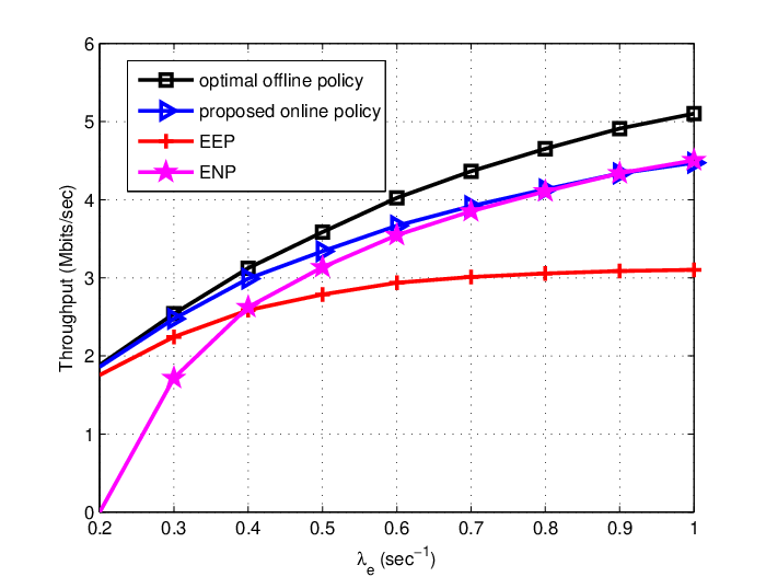


First, we consider a single AWGN channel in Figs. 4 and 5 with the same channel parameters as for Example III.1. In Fig. 4, we show the average throughput over secs versus , with Joule (J). It is observed that when is small, the proposed online policy and EEP obtain similar performance as the optimal off-line policy. Since the average harvested energy is small when is small, it is more likely that is greater than both (c.f. (V-A)) and (c.f. (32)). Thus, both the proposed online and off-line policies choose to transmit with during the “on” periods to save energy. However, for ENP, the transmit power level deviates from and thus significant amount of energy is consumed due to the non-ideal circuit power; as a result, the achievable throughput is almost zero. As increases, the throughput gap between the optimal off-line policy and all online policies enlarges, and the performance of EEP degenerates severely. Moreover, ENP is observed to obtain a similar performance as the proposed online policy. This is because in this case, is negligibly small as compared with , and as a result the proposed online policy degenerates to ENP.
Fig. 5 shows the average throughput versus , for two different values of /sec and 1/sec, with J. In both cases of , the proposed online policy is observed to perform close to the optimal off-line policy, for all values of . With small value of , i.e., /sec, EEP performs much better than ENP since it is more energy efficient, while with a larger value of , i.e., /sec, the reverse becomes true, which can be similarly explained as for Fig. 4.
Furthermore, for the multi-channel scenario, in Fig. 6 we evaluate the average throughput of a single-cell downlink system with the base station (BS) powered by energy harvesting. It is assumed that the BS covers a circular area with radius 1000 meters, and serves users whose locations are generated following a spatial homogeneous Poisson point process (HPPP) with density users/m2. Consider a simplified channel model without fading, in which the channel power gain of each user from the BS is determined by a pathloss model , where dB is a constant equal to the pathloss at a reference distance m, and is the pathloss exponent. Assuming an OFDMA (orthogonal frequency division multiplexing access) based user multiple access, a total bandwidth MHz is equally allocated to the users. The noise power spectral density at each user receiver is set as dBm/Hz and is assumed. The circuit power at the BS is set as Watt. Fig. 6 shows the average throughput versus with J and an energy scheduling period 20secs. It is observed that the proposed online policy always performs better than EEP. With small values of , i.e., /sec, ENP preforms clearly worse than the proposed online algorithm, while when /sec, both schemes perform similarly. This observation is expected as can be similarly explained for Fig. 4.
VII Concluding Remarks
In this paper, we studied the throughput-optimal transmission policies for energy harvesting wireless transmitters with the non-ideal circuit power. We first obtained the optimal off-line solution in the single-channel case, which is shown to have a new two-phase transmission structure by unifying existing results on separately maximizing energy efficiency and spectrum efficiency. We then extended the optimal off-line solution to the general case with multiple AWGN channels subject to a total energy harvesting power constraint, by the technique of nested optimization. Finally, we proposed an online algorithm based on a closed-form off-line solution. It is shown by simulations that the proposed online algorithm has a very close performance to the upper bound achieved by the optimal off-line solution, and also outperforms other heuristically designed online algorithms.
After submission of this manuscript, we become aware of one interesting related work [19] that is worth mentioning. In [19], the throughput optimization in a single-channel energy harvesting communication system with battery leakage is introduced. The impact of battery leakage is very similar to that of the non-ideal circuit power considered in this paper; as a result, the optimal transmission policy developed in [19] is similar to the one proposed in Section III of this paper. One difference is that the optimal off-line policy in [19] is developed by decoupling the general multi-epoch problem into multiple equivalent single-epoch subproblems, while the same optimal policy in this paper is derived by decoupling the problem into only two subproblems (c.f. Appendix C). Compared with the solution in [19], the off-line policy in this paper reveals the optimal two-phase structure in which EE and SE optimizations are unified, and thus motivates our online policies, which are not given in [19].
Appendix A Proof of Lemma III.1
Denote the length of the on-period as and that of the off-period as , where . Without loss of generality, we only need to consider the case with on-period and off-period , since exchanging the power allocation at two different time instants in an epoch does not change the throughput and the energy constraint. Next, we prove that the transmit power should be constant during the on-period in an epoch by contradiction.
Suppose that the optimal allocated transmit power , where is not constant. Since is a strictly concave function, based on Jensen’s inequality, we have
| (41) |
and then
| (42) |
Thus, if we construct a new transmit power allocation as , we can achieve a larger throughput than that achieved by . Moreover, we verify that consumes the same total energy as in the th epoch, i.e.,
| (43) |
Therefore, based on (42) and (43), we conclude that cannot be optimal and thus Lemma III.1 is proved.
Appendix B Proof of Proposition III.1
To solve (9), we note that the third inequality constraint must be met with equality by the optimal solution, since otherwise the throughput can be further improved by increasing . Thus, by substituting into the objective function as well as the constraint , the problem becomes equivalent to finding
| (44) |
Consider first the following problem with the relaxed power constraint:
| (45) |
This problem has been studied in [7], where the globally optimal solution is known as the EE-maximizing power allocation, denoted by . It was also shown in [7] that given , is monotonically increasing with if , and monotonically decreasing with if . Thus, the solution of (44) is obtained as
| (46) |
Accordingly, the optimal on-period is given by
| (47) |
Proposition III.1 is thus proved.
Appendix C Proof of Theorem III.1
To prove Theorem III.1, we construct the following two sub-problems and for the power allocation optimization in the first epochs and the last epochs, respectively.
| (48) |
| (49) |
We will first prove that the solution given in Theorem III.1 is optimal for both and , and then prove that the optimal solutions for and are also optimal for (8).
Consider the throughput maximization problem , with the arrived energy at time over the horizon . We construct an auxiliary throughput maximization problem with the energy arrival at time over the same horizon as follows.
| (50) |
It is clear that the optimal throughput of is an upper bound on that of since any feasible solution of is also feasible for . Note that there is no energy arrived in for , so is indeed equivalent to a throughput maximization problem for the single-epoch case studied in Section III-B over a horizon . It can be easily verified based on (13) that ; thus, it follows after some simple manipulation that the optimal value of is and is attained by and . Meanwhile, for we can always construct a feasible solution based on (14), (15) and (16) by setting
| (51) |
It can be verified from (13) that the solution satisfying (51) is feasible for , and attains an objective value of , which is the same as the optimal value of . The gap between and is thus zero, and accordingly, the solution given in (14), (15) and (16) is optimal for .
Second, we prove that the solution in (17), (18) and (19) is optimal for Problem over the last epochs. First, we show by contradiction as follows. Suppose that the optimal solution contains an “off” period with , i.e., .
Due to the definition of (13), it follows immediately that
| (52) |
Therefore, we can always find a time duration with , and construct a new policy with . Note that we have chosen to be sufficiently small so that and . The energy consumed by during is , which is same as the initial policy . The throughput for the newly constructed policy and initial policy during are
and
respectively. Since , and is monotonically decreasing as a function of when , we conclude that . Therefore, the new policy achieves a higher throughput than the initial policy.
Moreover, we need to check that the new policy also satisfies the energy constraint as follows. If , or and are in the same epoch, it is evident that the energy constraint is satisfied. If we cannot find an interval latter than or in the same epoch as , i.e., all the allocated power prior to is smaller than , in this case based on (52), there must be some energy left at time . Since we selected to be sufficiently small, we can still guarantee that the energy constraint is satisfied. Therefore, we prove that .
After determining , we realize that Problem for the last epochs has the same structure as that studied in [12], and thus [12, Theorem 1] is applicable here. After some change of notation, we can prove that the solution in (17), (18) and (19) is optimal for over the last epochs.
Next, we show that the optimal solutions of and are optimal for (8) to complete the proof for Theorem III.1. First, we can verify by following the similar contradiction proof in the above that any energy harvested during should be used up in the first epochs, i.e., . Therefore, the energy constraint for (8) is equivalent to
| (53) |
Since the energy constraint is decoupled before and after , solving (8) is equivalent to optimizing and over and separately. Thus, the optimal solutions for and are also optimal for (8). Theorem III.1 is thus proved.
Appendix D Proof of Proposition IV.1
The first and third properties of can be directly verified by the first and third properties of , respectively. Thus, to complete the proof of Proposition IV.1, we only need to show the second property of , i.e., it is a strictly concave function of . Similar to [18, Appendix B], we show the proof of this result as follows.
Since is obtained as the optimal value of (26), which is a convex optimization problem and satisfies the Slater’s condition [17]. Thus, the duality gap for this problem is zero. As a result, can be equivalently obtained as the optimal value of the following min-max optimization problem:
| (54) | ||||
| (55) | ||||
| (56) |
where we have removed for brevity, and in (55) is the optimal solution for the maximization problem with a given , while in (56) is the optimal solution for the minimization problem with a given . Since is a strictly joint concave function, the optimal solutions in the above must be unique. Denote as any constant in . Let , and be the optimal for , and with , respectively. For , we have
| (57) | ||||
| (58) |
where strict inequality holds for (58) if since the optimal , are unique. Thus, we have
| (59) | ||||
| (60) | ||||
| (61) | ||||
| (62) |
where strict inequality holds for (60) if . Therefore, is a strictly concave function over . The proof of Proposition IV.1 is thus completed.
Appendix E Proof of Proposition V.1
We prove this proposition by considering the following two cases.
First, consider the case when exists, i.e., . In this case, setting as the transmit power at time 0 is optimal according to Table I. Furthermore, we have based on (13), and thus
Thus, (32) is equivalent to , which is the optimal solution.
References
- [1] T. Chen, Y. Yang, H. Zhang, H. Kim, and K. Horneman, “Network energy saving technologies for green wireless access networks,” IEEE Wireless Commun., vol. 18, no. 5, pp. 30-38, Oct. 2011.
- [2] C. Han et al., “Green radio: Radio techniques to enable energy-efficient wireless networks,” IEEE Commun. Mag., vol. 49, no. 6, pp. 46-54, Jun. 2011.
- [3] Z. Niu, Y. Wu, J. Gong, and Z. Yang, “Cell zooming for cost-efficient green cellular networks,” IEEE Commun. Mag., vol. 48, no. 11, pp. 74-78, Nov. 2010.
- [4] Z. Hasan, H. Boostanimehr, and V. Bhargava, “Green cellular networks: A survey, some research issues and challenges,” IEEE Commun. Surveys & Tutorials, vol. 13, no. 4, pp. 524-540, 2011.
- [5] Y. Chen, S. Zhang, S. Xu, and G. Y. Li, “Fundamental trade-offs on green wireless networks,” IEEE Commun. Mag., vol. 49, no. 6, pp. 30-37, Jun. 2011.
- [6] E. Uysal-Biyikoglu, B. Prabhakar, and A. Gamal, “Energy-efficient packet transmission over a wireless link,” IEEE/ACM Trans. Network., vol. 10, no. 4, pp. 487-499, Aug. 2002.
- [7] G. W. Miao, N. Himayat, and G. Y. Li, “Energy-efficient link adaptation in frequency-selective channels,” IEEE Trans. Commun., vol. 58, no. 2, pp. 545-554, Feb. 2010.
- [8] C. Isheden, Z. Chong, E. Jorswieck, and G. Fettweis, “Framework for link-level energy efficiency optimization with informed transmitter,” IEEE Trans. Wireless Commun., vol. 11, no. 8, pp. 2946-2957, Aug. 2012.
- [9] O. Blume, H. Eckhardt, S. Klein, E. Kuehn, and W. M. Wajda, “Energy savings in mobile networks based on adaptation to traffic statistics,” Bell Labs Tec. J., vol. 15, no. 2, pp. 77-94, Sep. 2010.
- [10] H. Kim and G. Veciana, “Leveraging dynamic spare capacity in wireless system to conserve mobile terminals energy,” IEEE/ACM Trans. Network., vol. 18, no. 3, pp. 802-815, Jun. 2010.
- [11] A. Kansal, J. Hsu, S. Zahedi, and M. B. Srivastava, “Power management in energy harvesting sensor networks,” ACM Trans. Embed. Comput. Syst., vol. 6, no. 4, Sep. 2007.
- [12] J. Yang and S. Ulukus, “Optimal packet scheduling in an energy harvesting communication system,” IEEE Trans. Commun., vol. 60, no. 1, pp. 220-230, Jan. 2012.
- [13] C. K. Ho and R. Zhang, “Optimal energy allocation for wireless communications with energy harvesting constraints,” IEEE Trans. Sig. Process., vol. 60, no. 9, pp. 4808-4818, Sep. 2012.
- [14] K. Tutuncuoglu and A. Yener, “Optimum transmission policies for battery limited energy harvesting nodes,” IEEE Trans. Wireless Commun., vol. 99, no. 2, pp. 1-10, Feb. 2012.
- [15] Q. Bai, J. Li, and J. A. Nossek, “Throughput maximizing transmission strategy of energy harvesting nodes,” in Proc. IWCLD, Rennes, France, Nov. 2011.
- [16] A. Goldsmith, Wireless Communications. Cambridge, U.K.: Cambridge Univ. Press, 2005.
- [17] S. Boyd and L. Vandenberghe, Convex Optimization, Cambridge University Press, 2004.
- [18] R. Zhang, F. Gao, and Y.-C. Liang, “Cognitive beamforming made practical: Effective interference channel and learning-throughput tradeoff,” IEEE Trans. Commun., vol. 58, no. 2, pp. 706-718, Feb. 2010.
- [19] B. Devillers and D. Gunduz, “A general framework for the optimization of energy harvesting communication systems with battery imperfections,” Journal of Commun. and Netw., vol. 14, no. 2, pp. 130-139, Apr. 2012.