Resistivity of non-Galilean-invariant Fermi- and non-Fermi liquids
Abstract
While it is well-known that the electron-electron (ee) interaction cannot affect the resistivity of a Galilean-invariant Fermi liquid (FL), the reverse statement is not necessarily true: the resistivity of a non-Galilean-invariant FL does not necessarily follow a behavior. The behavior is guaranteed only if Umklapp processes are allowed; however, if the Fermi surface (FS) is small or the electron-electron interaction is of a very long range, Umklapps are suppressed. In this case, a term can result only from a combined–but distinct from quantum-interference corrections– effect of the electron-impurity and ee interactions. Whether the term is present depends on 1) dimensionality [two dimensions (2D) vs three dimensions (3D)], 2) topology (simply- vs multiply-connected), and 3) shape (convex vs concave) of the FS. In particular, the term is absent for any quadratic (but not necessarily isotropic) spectrum both in 2D and 3D. The term is also absent for a convex and simply-connected but otherwise arbitrarily anisotropic FS in 2D. The origin of this nullification is approximate integrability of the electron motion on a 2D FS, where the energy and momentum conservation laws do not allow for current relaxation to leading –second–order in ( is the Fermi energy). If the term is nullified by the conservation law, the first non-zero term behaves as . The same applies to a quantum-critical metal in the vicinity of a Pomeranchuk instability, with a proviso that the leading (first non-zero) term in the resistivity scales as (). We discuss a number of situations when integrability is weakly broken, e.g., by inter-plane hopping in a quasi-2D metal or by warping of the FS as in the surface states of topological insulators of the Bi2Te3 family. The paper is intended to be self-contained and pedagogical; review of the existing results is included along with the original ones wherever deemed necessary for completeness.
I Introduction
00footnotetext: Submitted to a special issue of the Lithuanian Journal of Physics dedicated to the memory of Y. B. Levinson.A scaling of the resistivity with temperature () is considered as an archetypal signature of the Fermi-liquid (FL) behavior in metals. This result owes its origin to the Pauli exclusion principle which dictates that, at low temperatures, only those quasiparticles that reside within a width of order near the Fermi energy participate in binary collisions. This argument, however, applies only to the inverse of the quasiparticle relaxation time but not to the resistivity, , per se: the scaling of the former does not necessarily imply that of the latter. A very simple example is a Galilean-invariant FL, where the electron-electron (ee) interaction does not affect the resistivity, although , as measured, e.g., by thermal conductivity, does scale as . The reason is that, since velocities of electrons are proportional to their respective momenta, conservation of momentum automatically implies conservation of the electric current. In order to achieve a steady-state current under the effect of an external electric field, a momentum relaxation mechanism is needed.
Of course, the FL of electrons in a metal is not Galilean-invariant. In the presence of lattice, the current may be relaxed by Umklapp collisions, [1] which conserve the quasimomentum up to a reciprocal lattice vector: . Umklapp processes are allowed, however, if the incoming electron momenta and as well as the momentum transfer are all of order . These requirements are satisfied 1) if the Fermi surface is large enough, e.g., at least quarter-filled in the tight-binding case, [2] and 2) if the interaction is sufficiently short-ranged. In conventional metals, these two conditions are easily met due to a large number of carriers and effective screening of the Coulomb interaction; thus Umklapp collisions occur at a rate comparable to , and .
However, there are situations when these conditions are not met; e.g., the first condition is violated in systems with low carrier concentration, such as degenerate semiconductors, semimetals, surface states of three dimensional topological insulators, etc., and the second condition is violated when a metal is tuned to the vicinity of a Pomeranchuk-type quantum phase transition [3] (QPT), e.g, a ferromagnetic QPT. A Pomeranchuk-type QPT is a instability of the ground state, manifested by a divergence of long-wavelength fluctuations of the order parameter. The effective radius of the interaction mediated by the exchange of such fluctuations diverges at the QPT. One of the consequences of this divergence is the FL breakdown, as manifested by a non-Fermi–liquid (NFL) scaling with , but another one is the concurrent suppression of Umklapp processes.
If Umklapps are suppressed (and the temperature is too low for the electron-phonon interaction to be effective), current can be relaxed only via electron-impurity (ei) collisions. Still, the normal, i.e., momentum-conserving, ee collisions can affect the resistivity, if certain conditions are met. The main purpose of this paper is to summarize and analyze these conditions. The combined effect of normal ee and ei interactions does not necessarily lead to the dependence (or its NFL analog) of the resistivity. Whether this happens depends on three factors: 1) dimensionality [two dimensions (2D) vs three dimensions (3D)], 2) topology (simply vs multiply connected), and 3) shape (convex vs concave) of the Fermi surface (FS). The term is absent not only for a Galilean-invariant but, more generally, for an isotropic FL with a non-parabolic spectrum, as well as for anisotropic but quadratic spectrum. In 2D, the conditions are more stringent. In addition to cases mentioned above, the term is absent for a simply-connected and convex but otherwise arbitrarily anisotropic FS. The reason behind this is that the term arises from electrons confined to move along the FS contour such that, for the convex case, momentum and energy conservations are similar to the 1D case, where no relaxation is possible.
The issue of an interplay between normal ee and ei interactions has a long history, and it is beyond the scope of this paper to give a comprehensive review of the existing literature; some aspects relevant to 3D metals are reviewed in Ref. 4. Very briefly, the first notion that normal processes can affect the resistivity even in a single-band metal probably goes back to the paper by Debye and Conwell. [5] There is also a large body of work on normal collisions in multi-band metals, following the original paper by Baber, [6] both at the phenomenological (reviewed thoroughly in Ref. 7) and microscopic [8] levels. That momentum relaxation occurs differently in 2D as compared to 3D was pointed by Gurzhi, Kopeliovich, and Rutkevich, first for the electron-phonon[9] and then for the ee[10] interactions. Maebashi and Fukuyama [11] analyzed an interplay between normal and Umklapp collisions for an anisotropic 2D FS and found that the normal collisions do not give rise to a term as long as the FS is convex. Rosch and Howell (Ref. 12a) and Rosch (Ref. 12b) showed that a similar nullification happens for the term in the optical conductivity in a disorder-free 2D system. Chubukov and two of us (D. L. M. and V. I. Y.) generalized the analysis for a NFL near the Pomeranchuk QPT. [13] Scaling of the resistivity near a convex-to-concave transition was studied in Ref. 14. This paper expands on our recent works [13, 14] and provides some more details.
It is worth noting that the effects studied in this paper occur already within the semiclassical theory of transport that neglects quantum interference between ee and ei scatterings. Whether semiclassical description makes sense is one of the issues analyzed in the paper (cf. Sec. V.1): as a general rule, semiclassical effects can be considered separately from quantum-interference ones in the ballistic but not in the diffusive limit. Another effect not captured by the semiclassical Boltzmann equation (BE) is the viscous correction to the resistivity, discussed in Sec. V.2. The viscous correction is expected to be the leading contribution to the resistivity resulting from the ee interaction in the high-temperature, hydrodynamic regime, when the ee mean free path is sufficiently short.
The rest of the paper is organized as follows. We begin by formulating the problem in terms of the Boltzmann equation (BE) both for the FL and the NFL cases in Sec. II. In Sec. III, we solve the BE perturbatively with respect to ee scattering, which is an adequate approximation at low enough temperatures, and analyze various stituations mentioned above. In Sec. IV, we discuss the opposite limit of high temperatures, when the ee contribution to the resistivity saturates, and show that a true scaling regime, with an appreciable difference between the low and high temperature limits of the resistivity, does not exist in a single-band metal (Sec. IV.1). Such a regime is shown to exist for a two-band metal with very different masses (Sec. IV.2). In Sec. V, we analyze the limits of the validity of the results based on the semi-classical BE with respect to both quantum (Sec. V.1) and classical (Sec. V.2) correlations between ee and ei interactions. Our concluding remarks are presented in Sec. VI.
II Boltzmann equation: Generalities
II.1 Collision integral
The most straightforward way to find the effect of the ee interaction on the conductivity in the semi-classical regime is via the Boltzmann equation (BE) which, for the case of a time-independent and spatially-uniform external electric field , reads
| (1) |
where is the electron charge and is the distribution function. The collision integrals and on the right-hand side describe the effects of the ee and ei interactions, respectively. Explicitly,
| (2) |
and
where is a short-hand notation for , and and are the ei and ee scattering probabilities, correspondingly. For a weak electric field, the left-hand side of the BE reduces to , where is the electron group velocity and is the equilibrium distribution function, with prime denoting a derivative with respect to the electron energy, (measured from the Fermi energy). Linearizing the ee collision integral on the right-hand side with respect to the non-equilibrium correction to , defined as
| (4) |
one obtains[2]
| (5) | |||||
II.2 Pomeranchuk quantum criticality
In addition to the case of a generic FL, we will be also interested in a special but widely studied case of a FL near a Pomeranchuk-type QPT, [3] which breaks the rotational symmetry and/or topology of the FS but leaves the translational symmetries intact. Examples of such a QPT include ferromagnetic and electronic nematic transitions. [15] As opposed to, e.g., charge-density waves and antiferromagnets, both the ordered and disordered phases are spatially uniform, and the transition is manifested via the divergence of certain susceptibility at . Therefore, critical fluctuations near the QPT are long-ranged, and the effective interaction among electrons, mediated by these fluctuations, is of a long range as well. Since a FL is, in general, unstable with respect to long-range interaction, the quantum-critical region of the phase diagram near the QPT is characterized by manifestly non-Fermi liquid (NFL) properties, such as a divergence of the specific heat coefficient. However, the long-range nature of the effective interaction has another aspect; namely, small-angle scattering at critical fluctuations effectively prohibits Umklapp processes which, in the absence of disorder, are necessary to render the resistivity finite. [13] Therefore, the ee contribution to the resistivity can result only from an interplay between ei and normal ee collisions.
In this Section, we briefly summarize the properties of the simplest model describing a QPT of the Pomeranchuk type: the Hertz-Moriya-Millis (HMM) model. [16] In this model, electrons are assumed to interact via an effective potential proportional to the divergent susceptibility of the order parameter. Details of the effective interaction depend on whether instability occurs in the charge or spin channel but, for our purposes, it suffices to model the interaction by a scalar function
| (6) |
where is the density of states, is the “distance” to the critical point along the axis of the control parameter (pressure, doping, etc.), and is the radius of interaction in the critical channel. Since (6) can be derived, strictly speaking, only in the random-phase approximation, one needs to require that (Ref. 17). [Alternatively, one can assume that the coupling between electrons and critical fluctuations is weak; [18] results of these two approaches differ only by re-definition of parameters.] The imaginary part of results from Landau damping of critical fluctuations by itinerant electrons. The correlation length of critical fluctuations diverges at the QPT, where .
For the interaction in Eq. (6), the inverse quasiparticle lifetime (the imaginary part of the self-energy) behaves as for and as for . The energy scale separates the FL and NFL regions of the phase diagram. Since the momentum transfers are small in both regions ( for and for ), the transport scattering time is longer than the lifetime: . In the NFL region, ; in the FL regime, with a small prefactor. [19] The conventional wisdom was that “transportization” of the relaxation time was the only manifestation of the long-range nature of the interaction, so that the resistivity could simply be obtained by substituting the transport time into the Drude formula. [19, 20] This yields and in the NFL regions in 3D and 2D, correspondingly. The scaling of the resistivity is indeed close to what has been observed experimentally in a number of itinerant ferromagnets near a QPT. [21] The reasoning tacitly assumes, however, that Umklapp collisions are still present, and occur at a rate comparable to that for normal ones, so that the transport time for normal collisions gives a reasonable estimate for the Umklapp scattering time. As we have already pointed out at the beginning of this Section, this assumption is not satisfied for a long-range interaction. In the next Section, we will quantify this statement. Before we proceed further, some general comments on the HMM model are in order.
First, we are going to use the BE even in the NFL region of the QPT, where quasiparticles are not well defined, i.e., when . This seems to be inconsistent with the general criterion of the validity of the BE. [22] However, well-defined quasiparticles are not required for the BE to be valid in a special case, when the effective ee interaction can be treated in the Migdal-Eliashberg approximation, i.e., when the self-energy depends on the electron energy but not the momentum and vertex corrections are small. In this case, the BE can be derived in the Keldysh technique without any conditions on the parameter , as long as a much weaker condition is satisfied. [23] This argument, formulated first by Prange and Kadanoff for the electron-phonon interaction,[24] was used later by a number of researchers in a wider context, [25] and also applicable to NFL systems, given that they allow Migdal-Eliashberg description. Having said that, we come to the second point, which is that the Migdal-Eliashberg treatment of the HMM model, thought previously to be controllable at least in the approximation,[18] has recently been shown to break down beyond the second loop order. [26] While acknowledging this problem, we remark that the processes responsible for this breakdown are effectively 1D-like scattering events, in which both the initial and final fermions move along the same line. Although these processes are dangerous for the single-particle self-energy, their contribution to the conductivity should be reduced by at least the “transport factor”, which discriminates against small-angle scattering.
Once the BE is adopted, the difference between the FL and NFL regimes becomes formal: the dependence of the ee scattering probability on the energy transfer may be neglected in the former but not in the latter.
II.3 Matrix elements on a lattice: normal vs Umklapp processes

The interaction potential between electrons on a lattice depends on the coordinates of two electrons separately rather than on their relative coordinate; transforming to the center-of-mass and relative coordinates, , where is a periodic function of but not of (The time-dependence of the effective interaction is not essential for the analysis below, and will be omitted.) Consequently,
| (7) |
where is the reciprocal lattice vector and the volume of the system is put to unity. The matrix element of on the Bloch wave functions reads
| (8) |
Now we consider a long-range interaction, relevant for a FL near the Pomeranchuk instability. In this case, the matrix element is non-negligible only if the first argument of is as small as possible, which means that and :
| (9) |
We see that the condition for an Umklapp process becomes very stringent: [13] since , the momentum conservation condition can only be satisfied at special points, where and is just another reciprocal lattice vector. As Fig. 1a shows, this is only possible if and are located at the edges of the Brillouin zone (and the FS is open). The volumes (areas) around the special points are small–in proportion to a small momentum transfer . The corresponding scattering rate is smaller than the transport rate of ee collisions by a factor of . For HMM criticality, where , this implies that the contribution to the resistivity from the process depicted in Fig. 1a scales as , i.e., as in 3D and as in 2D. In both cases, the exponents are larger or equal than . This means that the NFL contribution to the resistivity is smaller (3D) or comparable (2D) to the FL () contribution, arising from Umklapp scattering in the channels that are not affected by the proximity to a QCP, e.g., from the charge channel in the vicinity of a magnetic instability. In addition, processes in Fig. 1a are, in fact, ”pseudo-Umklapps” because they can be viewed as normal processes on a closed (hole) FS. The ”real” Umklapps, shown in Fig. 1b, can occur only if the constraint of small momentum transfer is relaxed or else, near half-filling, when the “gap” between the FS and the edges of the Brillouin zone is small. Half-filling, however, is more likely to result in a finite- instability of the ground state, e.g., antiferromagnetism, rather than in a Pomeranchuk QTP. From now on, our analysis will be focused on normal ee collisions, the matrix element of which is given by Eq. (9) with . The corresponding scattering probability, averaged over spins of the initial states and summed over spins of the final states, reads
| (10) | |||||
has certain symmetries. First, we assume the microreversibility property
| (11) |
In addition, since electrons are indistinguishable,
| (12) |
Finally, combining (11) and (12), we obtain
| (13) |
With only normal ee collisions taken into account, the total electron momentum is conserved, i.e.,
| (14) |
II.4 General properties of the solution
Before proceeding with a more detailed analysis of the BE, we make a few general comments.
- 1.
“Hidden” phonons. The linearized form of the steady-state BE assumes implicitly that the electron-phonon interaction is also present in the system; otherwise, the total electron energy will increase indefinitely due to the work done by the electric field. As usual (see, e.g., Ref. 7), we assume that the temperature is low enough so that one can neglect a direct electron-phonon contribution to the resistivity (which requires that , where ’s are the transport scattering times for corresponding processes) but high enough so that, for a fixed electric field, the electron-phonon interaction can still equalize the electron and lattice temperatures (which requires that the work done by the electric field on the energy relaxation length is much smaller than the temperature).
- 2.
Parity of a non-equilibrium part of the distribution function. A linear in term in can be written as
(15) where contains explicitly only the effects of the ee and ei interactions. At low enough temperatures (as specified in the previous paragraph), the electron-phonon interaction shows up only in the next–quadratic–term and does not affect the resistivity directly. At even lower temperatures, when , ee scattering can be treated as a perturbation to ei scattering. In this case, is determined by the crystal symmetry and by the ei scattering probability and, without specifying both of them, no properties of can be further inferred. However, if the ei scattering probability satisfies the microreversibility condition, [7] i.e., , then is odd in . Indeed, reversing the sign of in the BE and relabeling , we obtain
(16) Using time-reversal symmetry (which is guaranteed in the absence of the magnetic field and magnetic order) and microreversibility, we see that . This is the property of the non-equilibrium distribution function we will be using later on. To simplify the presentation, we will first use a model form of the ei collision integral, namely, a relaxation-time approximation (cf. comment in Ref. 29), which allows for a closed-form solution, and then extend the proof for the general form of given by Eq. (15).
However, one has to keep in mind that, beyond the Born approximation, microreversibility is not a general principle but a consequence of two microscopic symmetries, i.e., symmetries with respect to time– and space-inversions, and is thus absent in non-centrosymmetric systems. [30]
- 3.
No disorder–no steady-state linear-response regime. Since the momentum is conserved in normal collisions, the collision integral (5) is nullified by a combination , where B is -independent but otherwise arbitrary. This means that there is no unique steady-state solution in the linear-response regime. Obviously, the steady-state solution is absent because the total momentum of the electron system (per unit volume), , increases with time. Indeed, restoring the time and spatial derivatives in the BE, multiplying it by and integrating over we obtain
(17) where . Integrating by parts in the right-hand side and taking into account that the number density , we obtain
(18) The left-hand side is just the continuity equation while the right-hand side is the total force per unit volume. Therefore, although the electron liquid is not, generally speaking, Galilean-invariant, it is accelerated as a whole by the electric field. (In a crystal, an increase of the momentum in time leads to Bloch oscillations of the current; the current averaged over time is equal to zero.) Therefore, one needs to invoke impurity scattering in order to render the problem well-defined. [31]
- 4.
No lattice–no term in the resistivity. Adding just disorder but no lattice does not give rise to a term in the resistivity. Notice that this statement is weaker than “the ee interaction does not effect the resistivity at all”, which is true if depends only on the scattering angle but not on the electron energy. The simplest case is that of point-like impurities, when , where is the density of states (per one spin component) and is a constant. In this case, the BE reduces to
(19) where is an average of the directions of . In the absence of lattice, and hence the electric current . Now one can multiply the BE equation by and integrate over , upon which –in accord with (14)– drops out, and obtain a relation between and directly, without solving for :
(20) The resuling conductivity does not contain any effects of the ee interaction, except for FL renormalizations of and .
The same is true if the scattering probability depends only on the angle between and . Parameterizing as
(21) we expand and over a complete basis set of, e.g., Legendre polynomials in 3D:
(22) where () is the angle between and (), and is an odd function of the polar angles that vanishes when substituted into the collision integral. In terms of angular harmonics, the BE reduces to
(23) with
(24) If does not depend on the electron energy, one proceeds in the same way as for point-like impurities, i.e., one obtains a direct relation between and by multiplying (23) by and integrating over . The resulting (Drude) conductivity contains the transport time but no effects of the ee interaction (again, up to FL renormalizations).
If does depend on the electron energy, as it is often the case for semiconductors, the integral does not reduce to the electric current, and one needs to solve for in order to find the conductivity. Since the ee interaction affects , the conductivity is also affected. However, as we show in Sec. III.3.3, the effect leads only to a term in the resistivity (or in 2D).
III Electron-electron contribution to the resistivity
III.1 Do normal ee collisions affect the resistivity?
It may seem that the reverse statement to the heading of item #4 in the previous Section (“no lattice-no term in the resistivity”) should be “a term in the resistivity occurs in the presence of both disorder and lattice“. Indeed, while disorder takes care of momentum relaxation, lattice breaks the Galilean invariance. As a result, , which means that momentum conservation does not imply current conservation, and one cannot obtain a relation between the current and the electric field without actually solving the BE. In general, therefore, one should expect a term in the resistivity. While it is really the case in 3D, it turns out that the conservation laws in 2D forbid the term for a convex and simply-connected but otherwise arbitrary FS.
III.2 Low temperatures: perturbation theory
In this Section, we discuss the case of low temperatures, when the ee collisions are less frequent than the ei ones. In this case, the ee contribution can be found via the perturbation theory with respect to . We begin with the simplest–isotropic– model for electron-impurity scattering, when the BE is given by (19). However, we keep the dependence of the ei relaxation time on the electron energy for the time being.
At the first step, we solve (19) with , which yields
| (25) |
Next, we substitute back into (19) and find a correction due to
| (26) |
The corresponding correction to the component of the conductivity tensor is given by
| (27) | |||||
Here, is the momentum transfer, is the surface (line) element of an isoenergetic surface (contour) at energy in 3D (2D), and is a vector measuring the change in the total “vector mean free path ” due to ee collisions. The energy transfer was introduced by re-writing the energy conservation law as . The scattering probability is now allowed to depend on . Using the symmetry properties of , one can cast (27) into a more symmetric form
| (28) | |||||
Now let us count the powers of in (28). Each of the three energy integrals (over , , and ) gives a factor of which, in a combination with the overall factor, already gives a dependence, as is to be expected for a FL. The result holds as long as the integral over does not introduce additional dependence. This is the case in the FL regime, when typical are of order of the ultraviolet cutoff of the problem, i.e., the smallest of the three quantities: the reciprocal lattice vector, a typical size of the FS, and the inverse radius of the ee interaction. In this case, the dependence of can be neglected. The energy dependence of contributes only to higher order terms in and we neglect it for the time being as well, so that with
| (29) |
being the change in the electron current due to ee collisions. Finally, since the integrals of the combinaton of the Fermi functions over energies already produce a factor of , electrons can be projected onto the FS in the rest of the formula. This means that one can drop in both -functions and perform the surface integrals over the FS.
We pause here to remark that neglecting in the -functions does not mean performing an expansion in , , etc. In fact, all quasiparticles energies (, , etc.) are equal to zero because the electrons were projected onto the FS! What it really means is that the -functions impose constraints on the angles between and (and and ) with electrons’ momenta being on the FS. Typical values of these angles are determined by the ratio of typical () to . In a system with a short-range interaction, , where is the lattice spacing; therefore, typical angles are of order unity. On the other hand, typical () are of order , and corrections to angles due to finite are small as long as , where is the bandwidth; the last condition is implied anyhow to be in the FL regime. If the interaction radius, , is much longer than both the lattice spacing and the Fermi wavelength, is small but in proportion to rather than to , while is still of order . This means that effective ultraviolet energy scale is reduced to , and the FL description is valid only at low energies, where the effect of a finite energy transfer on the kinematics of collisions is negligible. This can be illustrated for a simple example of the quadratic spectrum, when the angle between, e.g., and , satisfies . Neglecting is justified as long as . Notice that this simplification is valid even near QPT (cf. Sec. II.2), where the scaling dimensions of and are different: but . A characteristic temperature, below which the condition is satisfied, coincides with the scale below which the quasiparticle description breaks down, which is the regime of main interest for quantum phase transitions.
As another remark, typical may be different for different observables. What we said above is true for the leading term in the ee contribution to the electrical conductivity in all dimensions , because the small behavior of the integrand in (28) is regularized by the factors that vanish in the limit of . (This is analogous to the regularizing effect of the factor in a transport cross-section for elastic scattering.) However, when calculating the single-particle lifetime (the imaginary part of the self-energy)[32] and thermal conductivity[33] in 2D, one runs into infrared logarithmic divergences, which means that the infrared region of the momentum transfers () does contribute to the result. In those cases, neglecting in the -functions is not justified. (The subleading terms in the conductivity also require more care; see Sec. III.3.3 below.)
Coming back to the main theme, we focus now on the FL case, when one can also neglect in the scattering probability. After all these simplifications, the diagonal component of the conductivity reduces to
| (30) | |||||
where superscript indicates that the corresponding quantity is evaluated at the FS. Now the integrals over all energies can be performed with the help of an identity
| (31) |
and we obtain a term in the conductivity with a prefactor given by a certain average over the FS
Clearly, whether the leading correction to the residual conductivity indeed scales as depends on whether the integral over the FS is nonzero. Since the integrand is positive, the integral may vanish only if under the energy conservation constraints imposed by the - functions. As a simple check, we apply Eq. () for the Galilean-invariant case, when . In this case, , as it should be.
We now consider a more general situation, when the dependence of the scattering probability is important, which is the case, e.g., near a QPT. In this case only two out of the three energy integrals can be performed explicitly and, instead of Eq. (), we obtain
| (33) |
where
| (34) |
and is the Bose function. For the effective interaction from Eq. (6) at the QPT (), power counting of (33) gives , which coincides with the estimate based on the transport time (cf. Sec. II.2). As in the FL case, however, one needs to make sure that the prefactor is non-zero.
III.3 Cases when the leading term vanishes
III.3.1 Isotropic system with an arbitrary spectrum
The first case is that of an isotropic but otherwise arbitrary energy spectrum. Such a situation may arise due to relativistic effects. Another (pseudo-relativistic) example is weakly doped graphene with a negligibly small trigonal warping of the FS. Since is a function of only, the -function constraints in Eq. () imply that and . Then,
where . Notice that the second line in Eq. () is not an expansion in small but an exact relation. Substituting Eq. () (and similar expressions for and ) into , it is easy to see that vanishes identically. Thus, there is no correction to the resistivity of a non-Galilean-invariant but isotropic system. This result also holds for a general quadratic spectrum , in which case and .
Notice that, in contrast to the Galilean-invariant case (with ), when not only the term but all higher order terms are absent, higher order (, etc.) terms are non-zero for a non-parabolic spectrum.

III.3.2 Approximate integrability: convex and simply connected Fermi surface in 2D
Kinematics of ee collisions on a circular FS.
The fact that term in the resistivity is absent for an isotropic FS does not mean that it is necessarily present for an anisotropic FS. In fact, the term is also absent for a simply-connected and convex but otherwise arbitrary FS in 2D. [10, 11, 13]. Before considering the general case, however, let us study the simplest example of such a FS, i.e., a 2D circular FS with quadratic spectrum. Since this is just a Galilean-invariant case, we already know (cf. Sec. II.4) that the ee interaction has no effect on the resistivity. However, it is instructive to see in a geometrical way how the term vanishes–this will be useful for the subsequent analysis of the general case in 2D. Geometrically, one needs to find two initial momenta, and , belonging to the FS, such that the final momenta, and , also belong to the FS. As shown in Fig. 2, only three situations are possible: [34] 1) Cooper channel, when the total initial and, therefore, the total final momentum is equal to zero; 2) swapping of velocities, when the initial momentum of one the electrons coincides with the final momentum of another electron and vice versa, i.e., ; 3) no scattering- this is the trivial case where the initial and final momenta of individual electrons are the same. For all of these cases, and thus the term is absent. To see that these situations indeed exhaust all the possibilities, one can solve the momentum and energy conservation equations, i.e., and , subject to the additional constraint . This leads to two equations: and , where denotes the angle between the vectors and . The three possible solutions are: , corresponding to case 1); , corresponding to case 2); and for arbitrary and , corresponding to case 3).
Kinematics of ee collisions on a generic convex FS.
The situation described above is not specific to a circular FS in 2D but occurs also for a generic convex FS, see Fig. 3a. Indeed, introducing a new variable in () and using the time-reveral symmetry () and symmetries of the scattering probability, we obtain
| (36) |
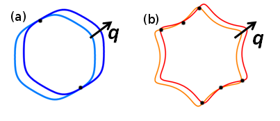
For given , we must find two momenta satisfying the relations and . Geometrically, finding the solution to these two equations is equivalent to shifting the FS by , and finding the points of intersection between the original and the shifted FSs. A convex FS has at most two self-intersection points. Therefore, the equation has only two solutions. In addition, if is a solution, then is also a solution so that the roots of the first equation form a set . Since the second equation is the same, its two roots must coincide with the roots of the first equation. This can happen if 1) , which gives the Cooper channel or if 2) which gives swapping. The situation with , when no scattering occurs, is trivially possible. For all the scattering processes listed above, and the term vanishes.
Being purely geometrical, the preceding analysis is equally valid for the NFL case, with the conclusion that the term vanishes as well.
Beyond the relaxation-time approximation.
Although the analysis above was based on Eq. (36), obtained in the relaxation-time approximation for ei scattering, it can be readily extended for the general form of the ei collision integral in Eq. (2). The non-equilibirum part of the distribution function in the presence of ei scattering only is given by (15), which implies that in (4) is replaced by . The lowest-order iteration in ee scattering is to be found from an integral equation
| (37) |
The ei collision integral can be viewed as an integral operator, the inverse of which is defined by
| (38) |
where . Thanks to microreversibility, . A formal solution of (37) is
| (39) |
Using the microreversibility property of and the fact that is odd in , it is easy to see that is odd in as well. This is all one really needs to repeat the steps of the previous analysis. The correction to the conductivity now contains a combination , where . Being odd in all momenta, behaves in the same way as upon the change . The scattering processes are classified in the same way as before, and the vanishing of the term follows from the vanishing of .
Approximate integrability.
A limited number of possible outcomes of the ee collisions means that our 2D system behaves similar to a 1D system, where binary collisions do not lead to relaxation. The analogy works because, to find the leading () term in the conductivity, it suffices to project electrons onto the FS, which is a line in 2D. Therefore, kinematics effectively becomes 1D and, although this is a 2D case, we have an integrable system. However, this analogy has certain limitations. First, the 2D case is integrable only with respect to charge but not thermal current relaxation, whereas there is no relaxation of all physical quantities in 1D. Second, even the charge current relaxation is absent only up to next-order-terms in (see Sec. III.3.3). Third, not any FS line in 2D is integrable: concave and multiply-connected contours behave in a non-integrable way. With all these limitations in mind, we will refer to the 2D convex case as to ”approximate integrability”.
III.3.3 Subleading corrections to the resistivity when the leading term is absent.
Higher order term from electrons away from the FS.
To find the subleading correction for the case considered in the previous section, we go back to Eq. (28), replace again by a constant in the scattering probability, but now, instead of neglecting in the functions, expand the product of the functions to second order in . The zeroth-order term, , nullifies . The odd in terms vanish upon integration over and In the FL case, this gives
| (40) | |||||
The derivatives of the -functions produce the same roots for and as the -functions themselves. However, integrating by parts, we make the derivatives to act on Although vanishes for and satisfying energy and momentum conservations, its derivatives do not. This makes the integral non-zero. Since we now have two more factors of the correction to the conductivity scales as
| (41) |
In more detail, let be one of the roots of the equation The corresponding root for is then Expanding around the roots gives
| (42) |
where and . Subsequent integration proceeds as in the integral
| (43) |
where and play the roles of and (and similarly for an integral with a product ). Further cancelations for a particular FS may make the dependence even weaker but the generic answer is
Clearly, going away from the FS produces an extra factor of . Since in the NFL as well, the result for the NFL regime is obtained by multiplying the “naive” estimate by , which gives . This is obviously subleading to the term resulting from the FL interaction in non-critical channels.
Energy-dependent electron-impurity relaxation time.
In addition to the mechanism described above, there are other sources of higher than corrections to the conductivity; one of them is the energy dependence of which we have neglected so far. This mechanism operates even in a Galilean-invariant system: although ee collisions conserve the momentum, they redistribute electrons in the energy space and thus affect the conductivity, if depends on the energy. [5, 7] To estimate the magnitude of this effect, we apply Eq. (28) to the Galilean-invariant case () and expand the impurity relaxation times entering the “vector mean free path” as , where . This yields
| (44) |
Since (27) contains two factors of , and each of them is proportional to , we have an extra factor in the integrand. In 3D, this immediately gives a term
| (45) |
In 2D, the situation is more delicate because the part of the integrand associated with the term in (44) is logarithmically divergent. This a well-known “2D log singularity” that occurs, on a more general level, as the mass-shell singularity of the self-energy (see Ref. 32 and references therein). This is also the same singularity that one encounters when calculating the thermal conductivity in 2D (in the absence of impurity scattering). [33] Indeed, our problem bears a formal similarity to that of the thermal conductivity because the change in the thermal current due to ee collisions
contains the same term as in (44). The singularity can be resolved by the same method as in Ref. 33. i.e., by considering a dynamically screened Coulomb interaction. The result is that, similar to the thermal conductivity, the conductivity contains an extra log factor as compared to the 3D case:
| (47) |
The “2D log” does not occur in the term in the conductivity, if the latter is finite due to broken integrability, which is the subject of the next section.
An extension to the NFL case is again, trivial, and we will not repeat the argument here.
III.4 Non-integrable cases
Concave FS in 2D.
It follows from the previous discussion that whether the term is absent or present depends entirely on the FS having two or more than two self-intersection points. A concave FS in 2D can have more than two self-intersection points (cf. Fig. 3b), therefore there are more than two solutions for the initial momenta for given . Some of these solutions still correspond to ”integrable” processes, encountered already for a convex FS, but the remaining ones do relax the current. Therefore, a term survives in this case.

3D FS.
In 3D, the manifold of intersection between the original and shifted FSs is a line, see Fig. 4(a). Therefore, the equation has infinitely many roots. There is no correlation between the roots of the equations and . Geometrically, this means that the initial momenta, and , do not have to be in the same plane as the final ones, and . Therefore, an anisotropic (but not quadratic) FS in 3D allows for a correction to the resistivity.
The term in the NFL regime survives for the same reason as well. Therefore, our theory at least does not contradict the experiments [21] where such term was observed.
Multiply connected FS.
If the FS is multiply connected, a term in the resistivity is present, even if the individual FS sheets do not allow for a term on their own. Even more so, the individual sheets can even be isotropic. The reason is obvious from Fig. 4(b) which shows an example of two circular FSs in 2D. Clearly, the equation has more than two roots even in this case. Thus, according to our previous arguments, there is no general reason for the vanishing of the term in such a situation. In Sec. IV and Appendix A, we discuss the two-band case in 2D in more detail.
III.5 Weakly-integrable cases
In this section, we consider two situations when integrability is broken only weakly.
III.5.1 Quasi-2D metal
The first case is a layered metal with a quasi-2D spectrum which, for simplicity, we assume to be separable into the in- and out-of-plane parts as
| (48) |
where and are the in-plane and out-of-plane components of the momentum, correspondingly. In the tight-binding model with nearest-neighbor hopping, , where is the lattice spacing in the -direction. The metal is in a quasi-2D regime when . In regard to the in-plane part of the spectrum, , we assume that the corresponding energy contours are anisotropic but convex so that, in the absence of inter-plane hopping, the -term in the in-plane conductivity would be absent. (If the planes are assumed to be Galilean-invariant, i.e., , as in a “corrugated cylinder model”, the -term is trivially zero because the in- and out-of-plane components of the momentum are conserved independently, and hence .) To find the -term in the in-plane conductivity, we use a method similar to that in Sec. III.3.3, i.e., we expand the -functions, except for that now we expand both in and . As we explained in Sec. III.2, the expansion in is really an expansion in normalized by the appropriate ultraviolet energy scale of the problem. Likewise, the expansion in is really an expansion in , which is a natural small parameter for a quasi-2D system. The zeroth-order term (, ) nullifies . The first-order terms also vanish: the ones, proportional to , do so by parity, and the ones, proportional to , do so because the first-order derivatives of the -functions nullify after a single integration by parts. Finally, the cross products in second-order terms, being odd in , also vanish. Therefore, the only surviving second-order term is
| (49) | |||||
Equation (49) contains two independent corrections. All terms proportional to produce a correction to the conductivity that exists even in a purely 2D system. All terms containing the squares of the out-of-plane dispersions produce a correction. [10] Therefore,
| (50) |
where , and constants and depend on details of the in-plane spectrum; generically, . Equation (50) describes a dimensional crossover from the 2D-like regime () at to the 3D-like regime () for . Notice that, in the 3D regime, the -term in the in-plane conductivity depends on the out-of-plane hopping.
In the NFL regime, Eq. (50) is replaced by
| (51) |
III.5.2 Conductivity near the convex-concave transition
In this Section, we consider a FS near a convex-concave transition which occurs when the Fermi energy goes above a certain threshold value . [14] Such a situation is encountered, e.g., in the case of surface states of the Bi2Te3 family of 3D topological insulators, where the electron spectrum can be approximated by[35] , with being the polar angle. Corresponding isoenergetic contours are shown in Fig. 6(a). We will be interested in the vicinity of the convex/concave transition, when .
We first consider the case of , when the isoenergetic contours near the Fermi energy are concave and thermal population of concave isoenergetic contours can be neglected. Obviously, in Eq. (36) shows a critical behavior: it is zero on the convex side and non-zero on the concave side of the transition. However, there are two other quantities which also show a critical behavior. As Figs. 5(a) and 5(b) illustrate, even a concave FS does not necessarily have more than two self-intersection points: this happens only if the FS is shifted along certain directions that lie close to high symmetry axes, i.e., lies within some angular interval , and the magnitude of the shift is below certain threshold, i.e., . Obviously, and also depend on in a critical manner. [36] Approximating by , we resolve the functions and integrate over all energies to obtain
where the sum runs over all intersection points, the prime denotes a derivative with respect to the polar angle, and . The task at hand now is to find the energy dependences of and .

This task is facilitated by the geometrical construction in Fig. 6(b). Let be the angle between the normal to the FS at a point, parameterized by the angle , and . As one goes around the FS contour, changes with . Figure 6(c) shows the dependence of on for the FS in Fig. 6(b) in the convex (, dotted), critical (, dashed), and concave (, solid) regimes. The dependence is monotonic for the convex FS and non-monotonic for the concave one. (This behavior is not specific to the particular FS considered here but is a general feature of any convex or concave contours). The oscillations are related to the rotational symmetry of the FS (six-fold in our case; Fig. 6(c) shows only the domain ). The non-monotonic parts are centered around special (“invariant”) points passed by the curves for all types of contours. Near the invariant points, the non-monotonic part of the curve obeys a cubic equation
| (53) |
where and is a constant. The energy dependences of the critical quantities can be obtained from this equation.
To find , we note that the equation reduces to for small . This implies that the solutions are those points on the FS where the normal to the FS is perpendicular to [cf. Fig. 6(b)], i.e., , where is the angle defining the direction of . From symmetry, if is a solution, so is ; therefore, one needs to consider only half the domain of . That only certain directions of allow for more than one solution to this equation, may be appreciated by inspecting Fig. 6(c), which makes it obvious that multiple roots can only occur in the regions of non-monotonicity. The interval where it happens is then proportional to the (vertical) width of these regions. Using Eq. (53), we find that . Similarly, one can show [14] that and (a posteriori, this justifies the assumption of small ).

Substituting these results into the expression for the conductivity, we find that , which means the prefactor of the term in the resistivity scales as . The term is always present, as discussed before. Hence, the resistivity has the following form:
| (54) |
where is the residual resistivity, is the step function, and and are material-dependent parameters (generically, ). A crossover between the and regimes occurs at .
Returning to the case of , when both convex and concave contours are populated, it is easy to see that the prefactor is replaced by , leading to a term in . This term, however, is subleading to the one. Therefore, Eq. (54) describes the leading -dependence of the resistivity in both situations ( and ) near the transition. Note that the exponents of , , and in Eq. (54) are universal, i.e., they are the same for an arbitrary 2D Fermi surface with a non-quadratic energy spectrum near a convex-concave transition.
IV High-temperature limit
So far, our analysis has been focused on the low-temperature limit, when the ee contribution to the resistivity is a correction to the ei one. From the experimental point of view, however, it is important to understand whether the ee contribution may become larger than the ei one. It is the case for Umklapp scattering, whose contribution grows unabated up to the temperatures comparable to the Fermi energy. The normal contribution, however, is different: it saturates in the limit when the ee relaxation time becomes shorter then the ei one. The effect of saturation was understood already in the earlier days of the electron transport theory:[37, 38] very frequent ee collision establish a quasi-equilibrium state with the drift velocity fixed by ei scattering. The previous analysis was, however, limited to the case when normal ee collisions affect the resistivity via the energy dependence of the ei relaxation time.[39, 7] In the next Section, we show that the saturation occurs even if the ei relaxation time does not depend on energy.
IV.1 Saturation of the resistivity in a single-band metal
We adopt the simplest model of point-like impurities with energy-independent scattering time, when the BE is given by Eq. (19). The ee collision integral in (19) can be viewed as a linear operator acting on the non-equilibrium part of the distribution function
| (55) |
The non-Hermitian matrix operator can be represented in terms of its left, , and right, , eigenstates as
| (56) |
where is the effective ee scattering time. The right and left states constitute an orthonormal basis:
| (57) |
where is the system volume in the D-dimensional space. A general solution of Eq. (19) can be expanded over the complete basis as
| (58) |
substituting this form into Eq. (19), we obtain an equation for the coefficients :
| (59) |
Only the zero mode () contribution survives in the limit of , so the solution in the high- regime is given by
| (60) |
It is not difficult to see that the right and left zero modes of are
| (61) |
Indeed,
| (62) |
due to momentum conservation; while
| (63) |
because the collision integral, evaluated for equilibrium distribution functions, remains to be equal to zero if all energies are shifted as with being an arbitrary -independent vector. The zero modes form a -dimensional subspace labeled by the Cartesian indices [ summation over these indices is implied in (58) and (60)]. The scalar product (57) of the zero-modes (61) is
| (64) | |||||
where
| (65) |
The scalar product (64) is diagonal in the coordinate system associated with the principal axes of the quadratic form ; normalization is ensured by choosing . Using these properties, we reduce Eq. (60) to
| (66) | |||||
Finally, we obtain the conductivity tensor in the high- limit as
| (67) |
In the opposite limit of low temperatures, the standard expression reads
| (68) |
In contrast to the case of energy-dependent , when the low- and high-temperature limits of the conductivity differ in how is averaged over the energy, [39, 7] these limits in our case differ in how the conductivity is averaged over the FS. Naturally, the two limits coincide for the Galilean-invariant case. Notice that saturation holds for any dimensionality and shape of the FS, i.e., regardless of whether the temperature dependences of the resistivity starts with a or term at low temperatures, it will saturate at high temperatures. In reality, of course, other scattering mechanisms, such as electron-phonon scattering, will mask the resistivity saturation.
If the FS is not abnormally anisotropic, the low- and high- limits are of the same order, which means that a true -scaling regime does not have room to develop. A mechanism in which such a regime is possible is considered in the next Section.
IV.2 Two-band model: Scaling regime
In this Section, we consider a simple model of a two-band metal with impurities. Since normal ee collisions affect the resistivity for any multiply-connected FS, we consider the simplest case of two bands with quadratic dispersions, , and, in general, different impurity scattering times, and We consider only the inter-band interaction (the intra-band one drops out in this case anyway) and neglect processes in which electrons are transferred from one band to another. The BE for this model in 2D can be solved exactly by generalizing the method of Appel and Overhauser [8](see Appendix A) with the result
| (69) |
where
| (70) |
and . The result for the resistivity follows already from the equations of motion[7]
| (71) |
if the phenomenological “friction coefficient” is expressed via the microscopic scattering time as .
An interesting case is when the masses are significantly different (as would be the case for a metal with partially occupied s and d bands [40]), e.g., and consequently, . At , the two bands conduct in parallel, and the total resistivity is dominated by that of the lighter band
| (72) |
At the resistivity saturates at a value determined by the resistivity of the heavy band
| (73) |
Therefore, the and limits now differ significantly
| (74) |
The scaling regime, in which
| (75) |
occurs in a wide temperature interval , the boundaries of which are defined by
| (76) |
This model can also be applied to the QPT, in which case it is natural to assume that critical fluctuations occur only in the heavy band. Consequently, the effective interaction is obtained from Eq. (6) by replacing and . Computing the integral (70) for and , we find the effective scattering rate in the NFL regime
| (77) |
where and are the Riemann and -functions, correspondingly. In this scenario, normal ee collisions do lead to a real scaling regime in the resistivity with an exponent given by “naive” power-counting argument.
V Limitations of the Boltzmann-equation approach
The semiclassical BE does not capture two types of effects. The first type–quantum– results from quantum interference between ee and ei scattering; the second one –classical–from correlations in the electron flow patterns produced by different impurities. In this section, we discuss the limits of validity of the semiclassical approach focusing on the 2D case.
V.1 Quantum-interference effects
V.1.1 Fermi-liquid regime
Recall that the FL-like contribution to the resistivity, discussed in this paper, behaves as (or , if there is approximate integrability) in the low-temperature regime, defined by and saturates in the high-temperature regime, defined by . In non-integrable systems, , where is the dimensionless coupling constant. In a generic FL, and the crossover between the two limits occurs at . For a good metal, so that . In case of quantum corrections (QC), the scale that differentiates between low and high temperatures, i.e., between the diffusive and ballistic regimes, is . For , one is in the diffusive limit, characterized by a logarithmically divergent Altshuler-Aronov correction; [41] with all coupling constants being of order one, , where is the Drude conductivity. For , one is in the ballistic limit, where the correction scales linearly with : (Ref. 42). Apart from the interaction correction, there is a also a weak-localization correction , where is the phase-breaking time, a precise form of which depends on whether one is in the diffusive or ballistic limits: in the former, ; in the latter, . In the diffusive limit, the weak-localization correction is similar to the Altshuler-Aronov result, differing only in the prefactor. In the ballistic limit, the weak localization correction is smaller than the interaction correction by a factor of . Therefore, the correct order of magnitude for the quantum-interference correction is still given by the interaction correction both in the diffusive and ballistic limits. Comparing the FL-contribution to the quantum corrections, we find that and in the diffusive and ballistic limits, correspondingly. Therefore, it is meaningful to consider the FL contribution and neglect quantum-interfence processes in the ballistic but not in the diffusive limit. The interplay of different mechanisms is shown schematically in Fig. 7.
In the integrable case, the term in the resistivity vanishes and the FL correction scales as . In this case, the FL correction dominates over the quantum one only at temperatures well above the diffusion-ballistic crossover: . It is worth noting that the discussion of the experimental observations of quantum corrections in the ballistic regime has been so far limited to 2D electron gases in Si and GaAs heterostructures [44], with essentially circular FSs and almost parabolic spectra, where the FL contribution is expected to be very small. The FL contribution, however, is expected to play a dominant role in 2D systems with highly anisotropic FSs and non-parabolic spectra, such as the surface state in the topological insulators of the Bi2Te3 family, discussed in Sec. III.5.2.

V.1.2 Non-Fermi–liquid regime
In this section, we describe the interplay between the quantum-interference and direct ee contributions to the resistivity in the NFL–regime of a ferromagnetic quantum phase. For simplicity, we assume that the integrability is broken already in a single-band case by sufficiently strong concavity of the FS. In this case, one can simply calculate the transport time for scattering at critical spin fluctuations, described by the propagator (6) with , and substitute the result into the Drude formula. [19] This gives , where (we remind that is a control parameter of the HMM model). The temperature above which the NFL contribution saturates is now given by . The main difference between the FL– and NFL–regimes is that quantum criticality changes space-time (or energy-momentum) scaling: while in a FL, near QCP, where is the dynamical exponent ( in the HMM model). Therefore, the temperature of the diffusive-ballistic crossover, determined by the condition , where is a typical value of the momentum transfer in an ee collision, is replaced by (Ref. 43). In a clean system, where , is significantly smaller than in a FL, where , so that the ballistic regime continues down to much lower temperatures compared to the FL case, and we limit our analysis to this regime. (Lowering of in the vicinity of a ferromagnetic QCP becomes noticeable already in the FL regime. [42]) Another consequence of quantum-critical scaling is that the quantum correction in the ballistic regime near a QCP behaves as as opposed to : (Ref. 43). Comparing the NFL and QC contributions, we find that the NFL contribution dominates only at , where . A relative weakness of of the NFL contribution is due to small-angle scattering at long-wavelength critical fluctuations.
V.2 Viscous contribution to the resistivity
The statement that ee interaction does not contribute to the resistivity of a Galilean-invariant FL (cf. Sec. II.4 ) seems to contradict an intuitive notion that it is the viscosity of a liquid that defines its rate of flow. In a certain regime, indeed, the resistivity does depend on the viscosity of the electron liquid. [45, 46] This effect is not taken into account by the standard BE which neglects not only quantum but also classical correlations between scattering events. The ”viscous” contribution occurs at high enough temperatures, when the mean free path due to the ee interaction, , is smaller than at least the average distance between impurities, , where is the number density of impurities. [46] In this regime, the ei mean free path is the largest scale of the problem, which implies that the FL contribution–even if allowed due to anisotropy of the FS–has already saturated of at a value comparable to the Drude resistvity (cf. Sec. IV). Barring phonons, the viscous contribution is the only source of the dependence in this regime.
To estimate the magnitude of the viscous contribution, we consider, following Ref. 46, a flow of the electron liquid through a random array of spherical impurities. First, the impurity radius is assumed to be much larger than , so that a hydrodynamic description is applicable at all lengthscales. The force on one electron from all impurities is just the Stokes force , where is the dynamic viscosity, is the flow velocity, and is the electron number density. [An exact value of the numerical coefficient in depends on the boundary conditions for the velocity at the surface of the sphere[47] but will not be needed here.] In steady state, , which yields , and thus the viscous contribution to the resistivity is given by . In a FL, ; thus the viscous correction is of the insulating sign. On the other hand, the Drude resistivity resulting from scattering off the same impurities is . The viscous contribution is smaller than the Drude resistivity within the hydrodynamic regime: .
In 2D, the Stokes force from a disk-like impurity depends on only logarithmically: , where . [47] However, also contains instead of , so that the ratio is the same (up to a logarithm) as in 3D.
The situation is somewhat different for small impurities, because a force exerted by a small () sphere on a rarified gas depends not on the viscosity but on the gas-solid accommodation coefficients. [48] In 2D, the situation is further complicated vy the Stokes paradox. [47] Hruska and Spivak [46] showed that the viscous correction for small impurities in 2D is given by
| (78) |
where is the impurity scattering length and . Because of a large logarithmic factor, can, in principle, be comparable to .
VI Conclusions
The main purpose of this paper was to analyze the effect of ee interactions on the resistivity in the situation when Umklapp scattering of electrons can be neglected. Such a situation arises, e.g., in low-carrier density materials, as well as in metals near a QPT, where the effective interaction is of a long range. In such cases, the conventional dependence (or its analog in the NFL region near a QPT) of the resistivity on temperature is not guaranteed. Whether it is present depends on 1) dimensionality, 2) shape, and 3) topology of the FS. If the FS is quadratic or isotropic, there is no contribution to the resistivity. However, anisotropy is not sufficient to guarantee the dependence. In the case of a convex and simply connected FS in 2D, there is no dependence either. In such cases, the leading temperature dependence on resistivity due to ee interactions is in the FL region and in the NFL region. Also, if the FS changes its shape from convex to concave as a function of the filling fraction, the resistivity follows a universal scaling form near the convex-concave transition. In all other cases, the (or ) behavior is allowed, albeit only as a correction to the Drude resistivity. However, a true scaling regime (when the ee contribution is larger then the ei one) is possible for a quantum-critical two-band metal with substantially different band masses. Since a quantum-critical behavior is observed typically in multi-band metals with partially occupied d bands, we conjecture that the scaling of the resistivity observed in 3D ferromagnets [21] and subquadratic scaling in a quasi-2D metamagnet Sr3Ru2O7 [49] is due to the interaction between light and heavy carriers in these materials.
Acknowledgements.
Regrettably, this paper could not been discussed with Yehoshua B. Levinson (1932-2008), who contributed immensely to the field of electron transport in solids. Nevertheless, one of the authors (D.L.M.) had a privilege to learn firsthand about many of the issues addressed here from Levinson more than two decades ago. The reader may also notice that this paper frequently cites the classic monograph by Gantmakher and Levinson (Ref. 7), which in and of itself, speaks about Levinson’s legacy. We would like to thank A. Chubukov, who collaborated with us on many aspects of this work. Stimulating discussions with A. Finkelstein, A. Kamenev, M. Kargarian, S.-S. Lee, D. Loss, I. Paul, C. Pépin, M. Reizer, S. Sachdev, B. Spivak, and A. Varlamov are gratefully acknowledged . This work was supported by RFBR-12-02-00100 (V.I.Y.) and NSF-DMR-0908029 (D.L.M.)Appendix A Two-band model in 2D
In this Appendix we derive Eq. (69). The two coupled BEs (1 and 2 refers to the bands 1 and 2) read
| (79) |
where is the electron-electron collision integral for scattering between two electrons from the th and th band, and are the equilibrium distributions. Since in our model each of the bands is Galilean-invariant on its own, the intra-band ee interaction cannot affect the resistivity, and the corresponding parts of the collision integrals are not written down. Linearizing () in the same way as for the single-band case
| (80) |
we obtain
| (81) |
where
| (82) | |||||
and differs from in that the first integral goes over instead of . We seek for a solution in the following form
| (83) |
where are the constants that are to be determined. Multiplying the first and second BEs by and and integrating over and , correspondingly, we obtain for the left-hand sides
| (84) |
Similarly, the ei collision integrals, integrated over the corresponding momenta, reduce to
| (85) |
For a FL, the scattering probability may be assumed to depend only on the momentum transfer but not energy transfer. In this case, the integrals of ee collision integrals multiplied over reduce to
| (86) |
where
| (87) |
with , and differs from (86) by a factor of . [Integration over energies was performed with the help of Eq. (31).] Solving the system of linear equations and
| (88) |
we find
| (89) |
where the effective ee scattering time was introduced as
| (90) |
Using that the Fermi energy is same for both bands, i.e., that , we cast Eq. (90) into a different form
| (91) |
Once are found, one readily finds the electric current and arrives at the expression for the resistivity quoted in Eq. (69). An explicit expression for was derived in Ref. 50 for a special case of the “ overscreened” Coulomb potential. Our result for this case coincides with that in Ref. 50 up to a numerical coefficient.
In general, the ee scattering probability depends not only on but also on . In this case, the integrals over energies cannot be performed in a general form, and the expression for can only be reduced to the form quoted in Eq. (70). It should be stressed that the electron masses occurring in all equations of this section should be understood as bare rather than renormalized masses. This follows from the derivation of the BE in the Keldysh technique using the Migdal-Eliashberg approximation.
References
- [1] L. D. Landau and I. J. Pomeranchuk, Phys. Z. Sowjetunion 10, 649 (1936); Zh. Eksp. Teor. Fiz. 7, 379 (1937).
- [2] A. A. Abrikosov, Fundamentals of the Theory of Metals, (North-Holland, Amsterdam, 1988).
- [3] I. J. Pomeranchuk, Sov. Phys. JETP 8, 361 (1958).
- [4] J. Bass, W. P. Pratt, P. Schroeder, Rev. Mod. Phys. 62, 646 (1990).
- [5] P. P. Debye and E. M. Conwell, Phys. Rev. 93, 693 (1954).
- [6] W. G. Baber, Proc. Roy. Soc. London 158, 383 (1937).
- [7] V. F. Gantmakher and Y. B. Levinson, Carrier Scattering in Metals and Semiconductors (North-Holland, Amsterdam, 1987).
- [8] J. Appel and A. W Overhauser, Phys. Rev. B 18, 758 (1978).
- [9] R. N. Gurzhi, A. I. Kopeliovich, and S. B. Rutkevich, JETP Lett. 32, 336 (1980).
- [10] R. N. Gurzhi, A. I. Kopeliovich, and S. B. Rutkevich, JETP Lett. 56, 159 (1982); c) Adv. Phys. 36, 221 (1987).
- [11] a) H. Maebashi and H. Fukuyama, J. Phys. Soc. Japan 66, 3577 (1997); b) ibid. 67, 242 (1998).
- [12] a) A. Rosch and P. C. Howell, Phys. Rev. B 72, 104510 (2005); b) A. Rosch, Ann. Phys. 15, 526 (2006).
- [13] D. L. Maslov, V. I. Yudson, and A. V. Chubukov Phys. Rev. Lett. 106, 106403 (2011).
- [14] H. K. Pal, V. I. Yudson, and D. L. Maslov, Phys. Rev. B 85, 085439 (2012).
- [15] E. Fradkin, S. A. Kivelson, M. J. Lawler, J. P. Eisenstein, A. P. Mackenzie, Ann. Rev. Cond. Matt. Phys. 1, 153 (2010).
- [16] J. A. Hertz, Phys. Rev. B 14, 1165 (1976); T. Moriya, Spin Fluctuations in Itinerant Electron Magnetism (Spinger-Verlag, Berlin, New York, 1985); A. J. Millis, Phys. Rev. B 48, 7183 (1993).
- [17] M. Dzero and L. P. Gor’kov, Phys. Rev. B 69, 092501 (2004); D. L. Maslov and A. V. Chubukov, ibid. 79, 075112 (2009).
- [18] a) A. V. Chubukov, C. Pépin, and J. Rech, Phys. Rev. Lett. 92, 147003 (2004); b) J. Rech, C. Pépin, and A. V. Chubukov, Phys. Rev. B 74, 195126 (2006).
- [19] A. J. Schofield, Contemp. Phys. 40, 95 (1999).
- [20] L. Dell’Anna and W. Metzner, Phys. Rev. Lett. 98, 136402 (2007) [Phys. Rev. Lett. 103, 159904 (2009) (E)].
- [21] F. M. Grosche, C. Pfleiderer, G. J. McMullan, G. G. Lonzarich, and N. R. Bernhoeft, Physica B 206+207, 20 (1995); M. Nicklas et al., M. Brando, G. Knebel, F. Mayr, W. Trinkl, and A. Loidl, Phys. Rev. Lett. 82, 4268 (1999); P. G. Niklowitz, F. Beckers, G. G. Lonzarich, G. Knebel, B. Salce, J. Thomasson, N. Bernhoeft, D. Braithwaite, and J. Flouquet, Phys. Rev. B 72, 024424 (2005).
- [22] E. M. Lifshitz and L. P. Pitaevskii, Physical Kinetics, (Oxford, Pergamon Press, 1981).
- [23] J. Rammer and H. Smith, Rev. Mod. Phys. 58, 323 (1986).
- [24] R. E. Prange and L. P. Kadanoff, Phys. Rev. 134, A566 (1964).
- [25] See, e.g., M. J. Graf, D. Rainer, and J. A. Sauls, Phys. Rev. B 47, 12089 (1993).
- [26] S.-S. Lee, Phys. Rev. B 80, 165102 (2009); M. A. Metlitski and S. Sachdev, Phys. Rev. B 82, 075127 (2010); D. F. Mross, J. McGreevy, H. Liu, and T. Senthil, Phys. Rev. B 82, 045121 (2010); A.V. Chubukov, Physics 3, 70 (2010).
- [27] B. I. Sturman, Sov. Phys.-Uspekhi 27 881 (1984) [Usp. Fiz. Nauk 144, 497 (1984)].
- [28] Since Ref. 27 is not widely available, we take a liberty to reproduce its main message here: Some sources quote a different form of : . This form is incorrect: it does not follow from a microscopic theory and falsely predicts a possibility of non-linear evolution of the distribution function in a linear system. Under a more restrictive assumption of microreversibility, the non-linear terms cancel out and becomes correct.
- [29] Strictly speaking, the second term in the collision integral should contain the distribution function averaged over the directions of rather than the equilibrium distribution . However, this difference is immaterial to linear order in .
- [30] M. D. Blokh and L. I. Magarill, Sov. Phys. Solid State 22, 1327 (1080) [Fiz. Tverd. Tela 22, 2279 (1980)].
- [31] A well-known case when the resistivity is finite only due to normal ee collisions is a perfectly compensated semi-metal. [7] Undoped graphene is a special case of a compensated system with zero Fermi energy, where the conductivity is finite (and universal) at even in the absence of any scattering. [51]
- [32] S. Gangadharaiah, D. L. Maslov, A. V. Chubukov, and L. I. Glazman, Phys. Rev. Lett. 94, 156407 (2005); A. V. Chubukov, D. L. Maslov, S. Gangadharaiah, and L. I. Glazman, Phys. Rev. B 71, 205112 (2005).
- [33] A. O. Lyakhov and E. G. Mishchenko, Phys. Rev. B 67, 041304 (2003).
- [34] R. N. Gurzhi, A. N. Kalinenko, and A. I. Kopeliovich, Phys. Rev. B 52, 4744 (1995).
- [35] L. Fu, Phys. Rev. Lett. 103, 266801 (2009).
- [36] More than two points of intersection may be possible for large momentum transfers of . However, this leads to higher order terms in .
- [37] C. Herring and E. Vogt, Phys. Rev. 93, 693 (1956)
- [38] R. Keyes, J. Phys. Chem. Solids 6, 1 (1958).
- [39] V. F. Gantmakher and Y. B. Levinson, JETP 47, 133 (1978).
- [40] T. J. Ziman, Electrons and Phonons: The Theory of Transport Phenomena in Solids, (Oxford, 2001).
- [41] B. L. Altshuler and A. G. Aronov, in Electron-Electron Interactions in Disordered Systems, edited by A. L. Efros and M. Pollak (Elsevier, 1985), p. 1.
- [42] G. Zala, B. N. Narozhny, and I. L. Aleiner, Phys. Rev. B 64, 214204 (2001).
- [43] I. Paul, C. Pépin, B. N. Narozhny , and D. L. Maslov, Phys. Rev. Lett. 95, 017206 (2005); I. Paul, Phys. Rev. B 77, 224418 (2008).
- [44] B. Spivak, S. V. Kravchenko, S. A. Kivelson, and X. P. A. Gao, Rev. Mod. Phys. 82, 1743 (2010).
- [45] R.N. Gurzhi, Sov. Phys. JETP 17, 521 (1964).
- [46] M. Hruska and B. Spivak, Phys. Rev. B65, 033315 (2002).
- [47] L. D. Landau and E. M. Lifshits, Fluid Mechanics (Pergamon Press, Oxford 1987).
- [48] Ref. 22, p. 62.
- [49] R. S. Perry, K. Kitagawa, S. A. Grigera, R. A. Borzi, A. P. Mackenzie, K. Ishida, and Y. Maeno, Phys. Rev. Lett. 86, 2661 (2001); S. A. Grigera, R. S. Perry, A. J. Schofield, M. Chiao, S. R. Julian, G. G. Lonzarich, S. I. Ikeda, Y. Maeno, A. J. Millis, A. P. Mackenzie, Science 294, 329 (2001); S. A. Grigera,P. Gegenwart, R. A. Borzi, F. Weickert, A. J. Schofield, R. S. Perry, T. Tayama, T. Sakakibara, Y. Maeno, A. G. Green, A. P. Mackenzie, Science 306, 1154 (2004).
- [50] S. S. Murzin, S. I. Dorozhkin, G. Landwehr, and A. C. Gossard, JETP Lett. 67, 113 (1998).
- [51] A. W. W. Ludwig, M. P. A. Fisher, R. Shankar, and G. Grinstein, Phys. Rev. B 50, 7526 (1994); E. G. Mishchenko, Phys. Rev. Lett. 98, 216801 (2007).