The supernova-regulated ISM. I. The multi-phase structure
Abstract
We simulate the multi-phase interstellar medium (ISM) randomly heated and stirred by supernovae (SNe), with gravity, differential rotation and other parameters of the solar neighbourhood. Here we describe in detail both numerical and physical aspects of the model, including injection of thermal and kinetic energy by SN explosions, radiative cooling, photoelectric heating and various transport processes. With a three-dimensional domain extending horizontally and vertically (symmetric about the galactic mid-plane), the model routinely spans gas number densities –, temperatures 10–, local velocities up to (with Mach number up to 25). The working numerical resolution of 4 pc has been selected via simulations of a single expanding SN remnant, where we closely reproduce, at this resolution, analytical solutions for the adiabatic and snowplough regimes. The feedback of the the halo on the disc cannot be captured in our model where the domain only extends to the height of above the mid-plane. We argue that to reliably model the disc-halo connections would require extending the domain horizontally as well as vertically due to the increasing horizontal scale of the gas flows with height.
The thermal structure of the modelled ISM is classified by inspection of the joint probability density of the gas number density and temperature. We confirm that most of the complexity can be captured in terms of just three phases, separated by temperature borderlines at about and . The probability distribution of gas density within each phase is approximately lognormal. We clarify the connection between the fractional volume of a phase and its various proxies, and derive an exact relation between the fractional volume and the filling factors defined in terms of the volume and probabilistic averages. These results are discussed in both observational and computational contexts. The correlation scale of the random flows is calculated from the velocity autocorrelation function; it is of order 100 pc and tends to grow with distance from the mid-plane. We use two distinct parameterizations of radiative cooling to show that the multi-phase structure of the gas is robust, as it does not depend significantly on this choice.
Keywords:
galaxies: ISM – ISM: kinematics and dynamics – turbulence1 Introduction
The multi-phase structure of the interstellar medium (ISM) affects almost all aspects of its dynamics, including its evolution, star formation, galactic winds and fountains, and the behaviour of magnetic fields and cosmic rays. In a widely accepted picture (Cox & Smith, 1974; McKee & Ostriker, 1977), most of the volume is occupied by the hot (), warm () and cold () phases. The concept of the multi-phase ISM in pressure equilibrium has endured with modest refinement (Cox, 2005), e.g., deviations from thermal pressure balance have been detected (Kalberla & Kerp, 2009, and references therein). Dense molecular clouds, while binding most of the total mass of the interstellar gas and being of key importance for star formation, occupy a negligible fraction of the total volume (Kulkarni & Heiles, 1987; Kulkarni & Heiles, 1988; Spitzer, 1990; McKee, 1995, e.g.). The main sources of energy maintaining this complex structure are supernova (SN) explosions and stellar winds (Mac Low & Klessen, 2004, and references therein). The clustering of SNe in OB associations facilitates the escape of the hot gas into the halo thus reducing the volume filling factor of the hot gas in the disc, perhaps down to 10% at the mid-plane (Norman & Ikeuchi, 1989). The energy injected by the SNe not only produces the hot gas but also drives ubiquitous compressible turbulence in all phases, as well as driving outflows from the disc, associated with the galactic fountain or wind, as first suggested by Bregman (1980). Thus turbulence, the multi-phase structure, and the disc-halo connection are intrinsically related features of the ISM.
A comprehensive description of the complex dynamics of the multi-phase ISM has been significantly advanced by numerical simulations in the last three decades, starting with Chiang & Prendergast (1985), followed by many others including Rosen et al. (1993); Rosen & Bregman (1995); Vázquez-Semadeni et al. (1995); Passot et al. (1995); Rosen et al. (1996); Korpi et al. (1999); Gazol-Patiño & Passot (1999); Wada & Norman (1999); de Avillez (2000); Wada & Norman (2001); de Avillez & Berry (2001); de Avillez & Mac Low (2002); Wada et al. (2002); de Avillez & Breitschwerdt (2004); Balsara et al. (2004); de Avillez & Breitschwerdt (2005a);de Avillez & Breitschwerdt (2005b); Slyz et al. (2005); Mac Low et al. (2005); Joung & Mac Low (2006); de Avillez & Breitschwerdt (2007); Wada & Norman (2007); Gressel et al. (2008). Numerical simulations of this type are demanding even with the best computers and numerical methods available. The self-regulation cycle of the ISM includes physical processes spanning enormous ranges of gas temperature and density, and of spatial and temporal scales, as it involves star formation in the cores of molecular clouds, assisted by gravitational and thermal instabilities at larger scales, which evolve against the global background of transonic turbulence driven, in turn, by star formation (Mac Low & Klessen, 2004). It is understandable that none of the existing numerical models covers the whole range of parameters, scales and physical processes known to be important.
Two major approaches in earlier work focus either on the dynamics of diffuse gas or on dense molecular clouds. Our model belongs to the former class, where we are mainly concerned with the ISM dynamics in the range of scales of order –. Numerical constraints prevent us (like many other authors) from fully including the gravitational and thermal instabilities which involve scales of less than 1 pc. In order to assess the sensitivity of our results to the parameterization of radiative cooling, we consider models with thermal instability, but reduce its efficiency using a sufficiently strong thermal conductivity to avoid the emergence of structures that are unresolvable at our numerical resolution. The results are compared to models with no thermally unstable branch over the temperature range between the cold and warm phases. To our knowledge, no direct study addressing the difference between these two kinds of the cooling parameterizations has been made. We note, however, that Vázquez-Semadeni et al. (2000) compared their thermally unstable model to a different model by Scalo et al. (1998), who used a thermally stable cooling function. Similarly, de Avillez & Breitschwerdt (2004) and Joung & Mac Low (2006) compared results obtained with different cooling functions, but again comparing different models: here we compare models with different cooling functions but which are otherwise the same.
An unavoidable consequence of the modest numerical resolution available, if we are to capture the dynamics on scales, is that star formation, manifesting itself only through the ongoing SN activity in our model, has to be heavily parameterized. We do, however, ensure that individual supernova remnants are modelled accurately, since this is essential to reliably reproduce the injection of thermal and kinetic energy into the ISM. In particular, our model reproduces with high accuracy the evolution of supernova remnants from the Sedov–Taylor stage until the remnant disintegrates and merges into the ISM (Appendix B).
The dimensionless parameters characteristic of the ISM, such as the kinetic and magnetic Reynolds numbers (reflecting the relative importance of gas viscosity and electrical resistivity) and the Prandtl number (quantifying thermal conductivity), are too large to be simulated with current computers. Similarly to most numerical simulations of this complexity, our numerical techniques involve a range of artificial transport coefficients for momentum and thermal energy (such as shock-capturing viscosity). We explore and report here the sensitivity of our results to the artificial elements in our basic equations.
This paper is the first of a planned series, in which we aim to clarify which components and physical processes control the different properties of the ISM. Our next step is to add magnetic fields to the model, to study both their origin and role in shaping the ISM. But in order to identify where the magnetic field is important and where it is not, we first must understand what the properties of a purely hydrodynamic ISM would be.
The structure of the paper is as follows. In Section 2 we present our basic equations, numerical methods, initial and boundary conditions, as well as the physical ingredients of the model, such as our modelling of SN activity and heating and cooling of the ISM. Our results are presented in Sections 3–8, including an overview of the multi-phase structure of the ISM, the correlation length of random flows, and their sensitivity to the cooling function and numerical resolution. Our results are discussed in a broader context in Section 9, where our conclusions are also summarised. Detailed discussion of important technical and numerical aspects of the model, and the effects of the unavoidable unphysical assumptions adopted, can be found in Appendices: the accuracy of our modelling of individual supernova remnants in Appendix B, our control of numerical dissipation in Appendix C, and sensitivity to thermal instability in Appendix D.
2 Basic equations and their numerical implementation
2.1 Basic equations
We solve numerically a system of hydrodynamic equations using the Pencil Code (http://code.google.com/p/pencil-code) which is designed for fully nonlinear, compressible magnetohydrodynamic (MHD) simulations. We consider only the hydrodynamic regime for the purposes of this paper; MHD simulations, which are in progress, will be reported elsewhere. Nor do we include cosmic rays, which we subsequently plan to add to the MHD simulations.
The basic equations include the mass conservation equation, the Navier--Stokes equation (written here in the rotating frame), and the heat equation written in terms of the specific entropy:11 1 For the reader’s convenience, Appendix A contains a list of variables used in the text with their definitions.
| (1) | ||||
| (2) | ||||
| (3) |
where , and are the gas density, temperature and specific entropy, respectively, is the deviation of the gas velocity from the background rotation profile (here called the velocity perturbation), is the adiabatic speed of sound, is the heat capacity at constant pressure, is the velocity shear rate associated with the Galactic differential rotation at the angular velocity assumed to be aligned with the -axis (see below). The Navier–Stokes equation includes viscosity and the rate of strain tensor W whose components are given by
| (4) |
as well as the shock-capturing viscosity . The system is driven by SN energy injection, at the rates (per unit volume) in the form of kinetic energy in Eq. (2) and thermal energy in Eq. (3). Energy injection is applied in a single time step and is confined to the interiors of newly introduced SN remnants, and the total energy injected per supernova is denoted . The mass of the SN ejecta is included in Eq. (1) via the source . The forms of these terms are specified and further details are given in Section 2.2. The heat equation also contains a thermal energy source due to photoelectric heating , energy loss due to optically thin radiative cooling , heat conduction with the thermal diffusivity (with the thermal conductivity), viscous heating (with the determinant of W), and the shock-capturing thermal diffusivity .
The advective derivative,
| (5) |
includes transport by an imposed shear flow in the local Cartesian coordinates (taken to be linear across the local simulation box), with the velocity representing a deviation from the overall rotational velocity . As will be discussed later, due to anisotropies (e.g. density stratification, anisotropic turbulence), large-scale flows will be generated in the system; one example is the systematic vertical outflow discussed at length in this paper. Therefore, the perturbation velocity consists of two parts, a mean flow and random velocities. Here we consider a mean flow obtained by Gaussian smoothing (Germano, 1992):
| (6) | ||||
where we use a smoothing scale , necessarily somewhat shorter than the flow correlation length obtained in Section 6 (Gent et al., 2013, for details, see). The random flow is then . The differential rotation of the galaxy is modelled with a background shear flow along the local azimuthal () direction, . The shear rate is in terms of galactocentric distance , which translates into the -coordinate of the local Cartesian frame. In this paper we consider models with rotation and shear similar to those in the solar neighbourhood, . We do not expect the gas velocities and thermal structure discussed here to depend strongly on the rotation and shear parameters, although other aspects of the solution will be more sensitive to these. Future papers will consider the rotation and shear in more detail; and will also include magnetic fields, whose generation may depend strongly on these parameters.
We consider an ideal gas, with thermal pressure given by
where is the Boltzmann constant, is the proton mass, and is the mean molecular weight of a fully ionised gas of the Solar chemical composition.
In Eq. (2), is the gravitational potential produced by stars and dark matter. For the Solar vicinity of the Milky Way, Kuijken & Gilmore (1989) suggest the following form of the vertical gravitational acceleration (Ferrière, 2001, see also):
| (7) |
with , , and . We neglect self-gravity of the interstellar gas because it is subdominant at the scales of interest.
2.2 Modelling supernova activity
We include both Type II and Type I SNe in our simulations, distinguished only by their frequency and vertical distribution. The SNe frequencies are those in the Solar neighbourhood (Tammann, Löffler & Schröder, 1994, e.g.). Type II SNe are introduced at a rate, per unit surface area, of ( in the whole Galaxy), with fluctuations of the order of at a time scale of order . Such fluctuations in the Type II SN rate are natural to introduce; there is some evidence that they can enhance dynamo action in MHD models (Hanasz et al., 2004; Balsara et al., 2004). The surface density rate of Type I SNe is (interval of 290 years between Type I SN explosions in the Galaxy). We do not explicitly include any spatial clustering of the SNe.
Unlike most other ISM models of this type, the SN energy in the injection site is split between thermal and kinetic parts, in order to reduce artificial temperature and energy losses at early stages of the SN remnant evolution. Thermal energy density is distributed within the injection site as , with the local spherical radius and (of order – see below) the nominal location of the remnant shell (i.e. the radius of the SN bubble) at the time of injection. Kinetic energy is injected by adding a spherically symmetric velocity field ; subsequently, this rapidly redistributes matter into a shell. To avoid a discontinuity in at the centre of the injection site, the centre is simply placed midway between grid points. We also inject as stellar ejecta, with density profile . Given the turbulent environment, there are significant random motions and density inhomogeneities within the injection regions. Thus, the initial kinetic energy is not the same in each region, and, injecting part of the SN energy in the kinetic form results in the total kinetic energy varying between SN remnants. We therefore record the energy added for every remnant so we can fully account with the rate of energy injection. For example, in Model WSWa we obtain the energy per SN in the range
with the average of .
The SN sites are randomly distributed in the horizontal coordinates . Their vertical positions are drawn from the Gaussian distributions in with the scale heights of for Type II and for Type I SNe. Thus, Eq. (1) contains the mass source of per SN,
whereas Eqs. (2) and (3) include kinetic and thermal energy sources of similar strength adding up to per SN:
The only other constraints applied when choosing SN sites are to reject a site if an SN explosion would result in a local temperature above or if the local gas number density exceeds . The latter requirement ensures that the thermal energy injected is not lost to radiative cooling before it can be converted into kinetic energy in the ambient gas. More elaborate prescriptions can be suggested to select SN sites (Korpi et al., 1999; de Avillez, 2000; Joung & Mac Low, 2006; Gressel et al., 2008); we found this unnecessary for our present purposes.
Arguably the most important feature of SN activity, in the present context, is the efficiency of evolution of the SN energy from thermal to kinetic energy in the ISM, a transfer that occurs via the shocked, dense shells of SN remnants. Given the relatively low resolution of this model (and most, if not all, other models of this kind), it is essential to verify that the dynamics of expanding SN shells is captured correctly: inaccuracies in the SN remnant evolution would indicate that our modelling of the thermal and kinetic energy processes was unreliable. Therefore, we present in Appendix B detailed numerical simulations of the dynamical evolution of an individual SN remnant at spatial grid resolutions in the range –. We allow the SN remnant to evolve from the Sedov–Taylor stage (at which SN remnants are introduced in our simulations) for . The remnant enters the snowplough regime, with a final shell radius exceeding , and we compare the numerical results with the analytical solution of Cioffi et al. (1998). The accuracy of the numerical results depends on the ambient gas density : larger requires higher resolution to reproduce the analytical results. We show that agreement with Cioffi et al. (1998) in terms of the shell radius and expansion speed is excellent at resolutions for , and also very good at for and . Comparisons with models of higher resolution (de Avillez & Breitschwerdt, 2004; Joung et al., 2009), in Section 8.3, also indicate that our basic resolution is adequate.
Since shock waves in the immediate vicinity of an SN site are usually stronger than anywhere else in the ISM, these tests also confirm that our handling of shock fronts is sufficiently accurate and that the shock-capturing diffusivities that we employ do not unreasonably affect the shock evolution.
Our standard resolution is . To be minimally resolved, the initial radius of an SN remnant must span at least two grid points. Because the origin is set between grid points, a minimum radius of 7 pc for the energy injection site is sufficient. The size of the energy injection region in our model must be such that the gas temperature is above and below : at both higher and lower temperatures, energy losses to radiation are excessive and adiabatic expansion cannot be established. Following Joung & Mac Low (2006), we adjust the radius of the energy injection region to be such that it contains of gas. For example, in model WSWa this results in a mean of , with a standard deviation of and a maximum of . The distribution of radii appears approximately lognormal, so is very infrequent and the modal value is about ; this corresponds to the middle of the Sedov–Taylor phase of the SN expansion. Unlike Joung & Mac Low (2006), we found that mass redistribution within the injection site was not necessary. Therefore we do not impose uniform site density, particularly as it may lead to unexpected consequences in the presence of magnetic fields in our MHD simulations (described elsewhere).
2.3 Radiative cooling and photoelectric heating
| [K] | ||
|---|---|---|
| 10 | 2.12 | |
| 141 | 1.00 | |
| 313 | 0.56 | |
| 6102 | 3.21 | |
| 0.33 | ||
| 0.50 |
We consider two different parameterizations of the optically thin radiative cooling appearing in Eq. (3), both of the piecewise power-law form within a number of temperature ranges , with and given in Tables 1 and 2. Since this is just a crude (but convenient) parameterization of numerous processes of recombination and ionisation of various species in the ISM, there are several approximations designed to describe the variety of physical conditions in the ISM. Each of the earlier models of the SN-driven ISM adopts a specific cooling curve, often without explaining the reason for the particular choice or assessing its consequences. In this paper, we discuss the sensitivity of the results to the choice of the cooling function.
One parameterization of radiative cooling, labelled WSW and shown in Table 1, consists of two parts. For , we use the cooling function fitted by Sánchez-Salcedo et al. (2002) to the ‘standard’ equilibrium pressure–density relation of Wolfire et al. (1995, cf. Fig. 3b therein). For higher temperatures, we adopt the cooling function of Sarazin & White (1987). This part of the cooling function (but extended differently to lower temperatures) was used by Slyz et al. (2005) to study star formation in the ISM. The WSW cooling function was also used by Gressel et al. (2008). It has two thermally unstable ranges: at , the gas is isobarically unstable (); at , gas is isochorically or isentropically unstable ( and , respectively).
| [K] | ||
|---|---|---|
| 10 | 6.000 | |
| 300 | 2.000 | |
| 2000 | 1.500 | |
| 8000 | 2.867 | |
| 0.500 |

Results obtained with the WSW cooling function are compared with those using the cooling function of Rosen et al. (1993), labelled RBN, whose parameters are shown in Table 2. This cooling function has a thermally unstable part only above . Rosen et al. (1993) truncated their cooling function at . Instead of abrupt truncation, we have smoothly extended the cooling function down to . This has no palpable physical consequences as the radiative cooling time at these low temperatures becomes longer than other time scales in the model, so that adiabatic cooling dominates. The minimum temperature reported in the model of Rosen et al. (1993) is about . Here, with better spatial resolution, the lowest temperature is typically below .
We took special care to accurately ensure the continuity of the cooling functions, as small discontinuities may affect the performance of the code; hence the values of in Table 1 differ slightly from those given by Sánchez-Salcedo et al. (2002). The two cooling functions are shown in Fig. 1. The cooling function used in each numerical model is identified with a prefix RBN or WSW in the model label (see Table 3). The purpose of Models RBN and WSWb is to assess the impact of the choice of the cooling function on the results (Section 8.1). Other models employ the WSW cooling function.
We also include photoelectric heating in Eq. (3) via the stellar far-ultraviolet (UV) radiation, , following Wolfire et al. (1995) and allowing for its decline away from the Galactic mid-plane with a length scale comparable to the scale height of the stellar disc near the Sun (Joung & Mac Low, 2006, cf.):
This heating mechanism is smoothly suppressed at , since the photoelectric effect due to UV photon impact on PAHs (Polycyclic Aromatic Hydrocarbons) and small dust grains is impeded at high temperatures (Wolfire et al., 1995, cf.).
2.4 Numerical methods
2.4.1 The computational domain
We model a relatively small region within the galactic disc and lower halo with parameters typical of the solar neighbourhood. Using a three-dimensional Cartesian grid, our results have been obtained for a region in size, with in the radial and azimuthal directions and vertically on either side of the galactic mid-plane. Assuming that the correlation length of the interstellar turbulence is (see Section 6), the computational domain encompasses about 2,000 turbulent cells, so the statistical properties of the ISM can be reliably captured. We are confident that our computational domain is sufficiently broad to accommodate comfortably even the largest SN remnants at large heights, so as to exclude any self-interaction of expanding remnants through the periodic boundaries.
Vertically, our reference model accommodates ten scale heights of the cold Hi gas, two scale heights of diffuse Hi (the Lockman layer), and one scale height of ionised hydrogen (the Reynolds layer). The vertical size of the domain in the reference model is insufficient to include the scale height of the hot gas, and it would be preferable to consider a computational box of a larger vertical size, . Indeed, some similar ISM models use a vertically elongated computational box with the horizontal size of but the top and bottom boundaries at (e.g., de Avillez & Breitschwerdt, 2007, and references therein). However, the horizontal size of the domain in a taller box may need to be increased to keep its aspect ratio of order unity, so as to avoid introducing other unphysical behaviour at .
This constraint arises mainly from the periodic (or sliding periodic) boundary conditions in the horizontal planes as they preclude divergent flows at scales comparable to . However, the scale of the gas flow unavoidably increases with because of the density stratification. The steady-state continuity equation for a gas stratified in , , leads to the following estimate of the horizontal perturbation velocity arising due to the stratification:
| (8) |
where is the density scale height, , and is the horizontal scale of the flow, introduced via . Here we have neglected the vertical variation of , so that : this is justified for the hot and warm gas, since their vertical velocities vary weakly with at (see Fig. 12). Assuming for the sake of simplicity that is a constant, in Eq. (8), where is the horizontal correlation length of at , we obtain the following estimate of the horizontal correlation length at , the top of the domain:
where the time available for the expansion is taken as , is the horizontal correlation length of at . We find (Table 5) and (Fig. 19), so that the correlation scale of the velocity perturbation at the top and bottom boundaries of our domain, , follows as
Indeed, we find the correlation scale of the random flow increases to – at (Table 5), so that the diameter of the correlation cell, 400– becomes comparable to the horizontal size of the domain, . At larger heights, the periodic boundary conditions would suppress the horizontal flows, so that that the continuity equation could only be satisfied via an unphysical increase in the vertical velocity with . In addition, the size of SN remnants also increases with as the ambient pressure decreases. Thus, the gas velocity field (and other results) obtained in a model with periodic boundary conditions in and becomes unreliable at heights significantly exceeding the horizontal size of the computational domain.
The lack of a feedback of the halo on the gas dynamics in the disc can, potentially, affect our results. However, we believe that this is not a serious problem and, anyway, it would not necessarily be resolved by using a taller box of a horizontal size of only 1–. The gas flow from the halo is expected to be in the form of relatively cool, dense clouds, formed at large heights via thermal instability or accreted from the intergalactic space (Wakker & van Woerden, 1997; Putman et al., 2012, e.g.). A strong direct (as opposed to a long-term) effect of this gas on the multi-phase gas structure in the disc is questionable, as it provides just a fraction of the disc’s star formation rate, 0.1– versus 0.5– (Putman et al., 2012). Anyway, a taller computational domain would not help to include the accreted intergalactic gas in simulations of this type. In a galactic fountain, gas returns to the disc at a galactocentric distance at least away from where is starts (Bregman, 1980), and this could not be accounted for in models with tall computational boxes that are only 1– big horizontally.
In light of these concerns, and since it is not yet possible to expand our domain significantly in all three dimensions, we prefer to restrict ourselves to a box of height , thus retaining an aspect ratio of order unity. This choice of a short box requires great care in the choice of vertical boundary conditions (which might also introduce unphysical behaviour). We discuss our boundary conditions in detail in appendix C, but briefly note here that we use modified open boundary conditions on the velocity at . These conditions allow for both inflow and outflow, and so are to some extent capable of simulating gas exchange between the disc and the halo, driven by processes within the disc. More specifically, matter and energy are free to flow out of and into the computational domain across the top and bottom surfaces if the internal dynamics so require. (An inflow occurs when pressure beneath the surface is lower than at the surface or in the ghost zones).
2.4.2 Numerical resolution
For our standard resolution (numerical grid spacing) , we use a grid of (excluding ‘ghost’ boundary zones). We apply a sixth-order finite difference scheme for spatial vector operations and a third-order Runge–Kutta scheme for time stepping. We also investigate one model at doubled resolution, , labelled WSWah in Table 3; the starting state for this model is obtained by remapping a snapshot from the standard-resolution Model WSWa at Myr (when the system has settled to a statistical steady state) onto a grid in size.
Given the statistically homogeneous structure of the ISM in the horizontal directions at the scales of interest (neglecting arm-interarm variations), we apply periodic boundary conditions in the azimuthal () direction. Differential rotation is modelled using the shearing-sheet approximation with sliding periodic boundary conditions (Wisdom & Tremaine, 1988) in , the local analogue of cylindrical radius. We apply slightly modified open vertical boundary conditions, described in some detail in Appendix C, to allow for the free movement of gas to the halo without preventing inward flows at the upper and lower boundaries. In the calculations reported here, outflow exceeds inflow on average, and there is a net loss of mass from our domain, of order 15% of the total mass per Gyr. We do not believe that this slow loss of mass significantly affects our results
2.4.3 Transport coefficients
The spatial and temporal resolutions attainable impose lower limits on the kinematic viscosity and thermal diffusivity , which are, unavoidably, much higher than any realistic values. These limits result from the Courant–Friedrichs–Lewy (CFL) condition which requires that the numerical time step must be shorter than the crossing time over the mesh length for each of the transport processes involved. It is desirable to avoid unnecessarily high viscosity and thermal diffusivity. The cold and warm phases have relatively small perturbation gas speeds (of order ), so we prescribe and to be proportional to the local speed of sound, and . We ensure that the maximum Reynolds and Péclet numbers based on the mesh separation are always close to unity throughout the computational domain (see Appendix C): , and . This gives, for example, at and at . Thus, transport coefficients are larger in the hot gas where typical temperature and perturbation velocity are of order and , respectively. In all models , i.e., the Prandtl number . The corresponding fluid Reynolds and Péclet numbers, based on the correlation scale of the flow, fall in the range 20–40 in the models presented here.
Numerical handling of the strong shocks widespread in the ISM needs special care. To ensure that they are always resolved, we include shock-capturing diffusion of heat and momentum, with the diffusivities and , respectively, defined as
| (9) |
(and similarly for , but with a coefficient ), where denotes the maximum value occurring at any of the five nearest mesh points (in each coordinate). Thus, the shock-capturing diffusivities are proportional to the maximum divergence of the velocity in the local neighbourhood, and are confined to the regions of convergent flow. Here, is a dimensionless coefficient which we have adjusted empirically to 10. This prescription spreads a shock front over sufficiently many (usually, four) grid points. Detailed test simulations of an isolated expanding SN remnant in Appendix B confirm that this prescription produces quite accurate results, particularly those which are relevant to our goals: most importantly, the conversion of thermal to kinetic energy in SN remnants.
| (1) | (2) | (3) | (4) | (5) | (6) | (7) | (8) | (9) | (10) | (11) | (12) | (13) |
|---|---|---|---|---|---|---|---|---|---|---|---|---|
| Model | , C:W:H | |||||||||||
| [pc] | [] | [%] | ||||||||||
| WSWa | 4 | 1.8 | 3.9 | 2 : 60 : 38 | ||||||||
| WSWah | 2 | 1.8 | 0.5 | 3 : 51 : 46 | ||||||||
| RBN | 4 | 2.1 | 2.7 | 3 : 82 : 15 | ||||||||
| WSWb | 4 | 2.1 | 4.0 | 3 : 70 : 27 |
With a cooling function susceptible to thermal instability, thermal diffusivity has to be large enough as to allow us to resolve its most unstable normal modes:
where is the cooling function exponent in the thermally unstable range, is the radiative cooling time and is the adiabatic index. Figure 4 makes it evident that, in our models, typically exceeds 1 Myr in the thermally unstable regime. Further details can be found in Appendix D where we demonstrate that, with the parameters chosen in our models, thermal instability is well resolved by the numerical grid.
The shock-capturing diffusion broadens the shocks and increases the spatial spread of density around them. An undesirable effect of this is that the gas inside SN remnants cools faster than it should, thus reducing the maximum temperature and affecting the abundance of the hot phase. Having considered various approaches while modelling individual SN remnants in Appendix B, we adopt a prescription which is numerically stable, reduces gas cooling within SN remnants, and confines extreme cooling to the shock fronts. Specifically, we multiply the term in Eq. (3) by
| (10) |
where is the shock diffusivity defined in Eq. (9). Thus, almost anywhere in the domain but reduces towards zero in strong shocks, where is large. The value of the additional empirical parameter, , was chosen to ensure numerical stability with minimum change to the basic physics. We have verified that, acting together with other artificial diffusion terms, this does not prevent accurate modelling of individual SN remnants (see Appendix B).
2.4.4 Initial conditions
We adopt an initial density distribution corresponding to isothermal hydrostatic equilibrium in the gravity field of Eq. (7):
| (11) |
Since our present model does not contain magnetic fields or cosmic rays, which provide roughly half of the total pressure in the ISM (the remainder coming from thermal and turbulent pressures), we expect the gas scale height to be smaller than that observed. Given the limited spatial resolution of our simulations, the correspondingly weakened thermal instability and neglected self-gravity, it is not quite clear in advance whether the gas density used in our model should include molecular hydrogen or, alternatively, include only diffuse gas.
We used for models RBN and WSWb, corresponding to gas number density, at the mid-plane. This is the total interstellar gas density, including the part confined to molecular clouds. These models, discussed in Section 8.2, exhibit unrealistically strong cooling. Therefore, the subsequent models WSWa and WSWah have a smaller amount of matter in the computational domain (a 17% reduction), with , or , accounting only for the atomic gas (Joung & Mac Low, 2006, see also).
As soon as the simulation starts, density-dependent heating and cooling affect the gas temperature, so it is no longer isothermal and given in Eq. (11) is not a hydrostatic distribution. To avoid unnecessarily long initial transients, we impose a non-uniform initial temperature distribution so as to be near static equilibrium:
| (12) |
where is obtained from
The value of therefore depends on and the choice of the cooling function.

2.5 Models explored
We considered four numerical models, with relevant input parameters listed in Table 3, along with some output parameters describing the results. The models are labelled with prefix RBN or WSW according to the cooling function used. Angular brackets in Table 3 denote averages over the whole volume, taken from eleven snapshots (10 for WSWah) within the statistical steady state. The time span, , is given in Column 4, normalised by , where is the root-mean-square random velocity and is the horizontal size of the computational domain (e.g., in Model WSWa). As is set proportional to the speed of sound , it is variable and the table presents its average value , where and in all models. The numerical resolution is adequate when the mesh Reynolds number, , does not exceed a certain value (typically between 1 and 10) anywhere in the domain, where is the grid spacing (4 pc for all models, except for Model WSWah, where ). Therefore, we ensure that , where is the maximum perturbation velocity at any time and any grid point. The indicative values in Table 3 are averages of the mesh Reynolds number, , and the Reynolds number, . The Reynolds number based on the correlation scale of the random flow, , is thus 25 times larger than in all models explored here except for Model WSWah, where the difference is a factor of 50.
The quantities shown in Table 3 have been calculated as follows. In Column 9, the r.m.s. perturbation velocity is derived from the total perturbation velocity field , which excludes only the overall galactic rotation . In Column 10, the r.m.s. random velocity is obtained with the mean flows , defined in Eq. (6), deducted from . In Columns 11 and 12, and are the average thermal and kinetic energy densities, respectively; the latter includes the perturbation velocity and both are normalised to the SN energy . The values of the volume fractions of the cold, warm and hot phases (defined in Section 4) near the mid-plane are given in Column 13.
The reference model, WSWa, uses the WSW cooling function but with lower gas density than WSWb, to exclude molecular hydrogen (see Section 3). Model WSWah, which differs from WSWa only in its spatial resolution, is designed to clarify the effects of resolution on the results. We also analyze two models which differ only in the cooling function, RBN and WSWb, to assess the sensitivity of the results to this choice.
3 The reference model
Model WSWa is taken as a reference model; it has rotation corresponding to a flat rotation curve with the Solar angular velocity, and gas density reduced to exclude that part which would have entered molecular clouds. Results for this model were obtained by the continuation of the Model WSWb, in which the mass from molecular hydrogen had been included: at , the mass of gas in the domain was changed to that of Model WSWa by reducing gas density by at every mesh point. The effect of this change of the total mass is discussed in Section 8.2.
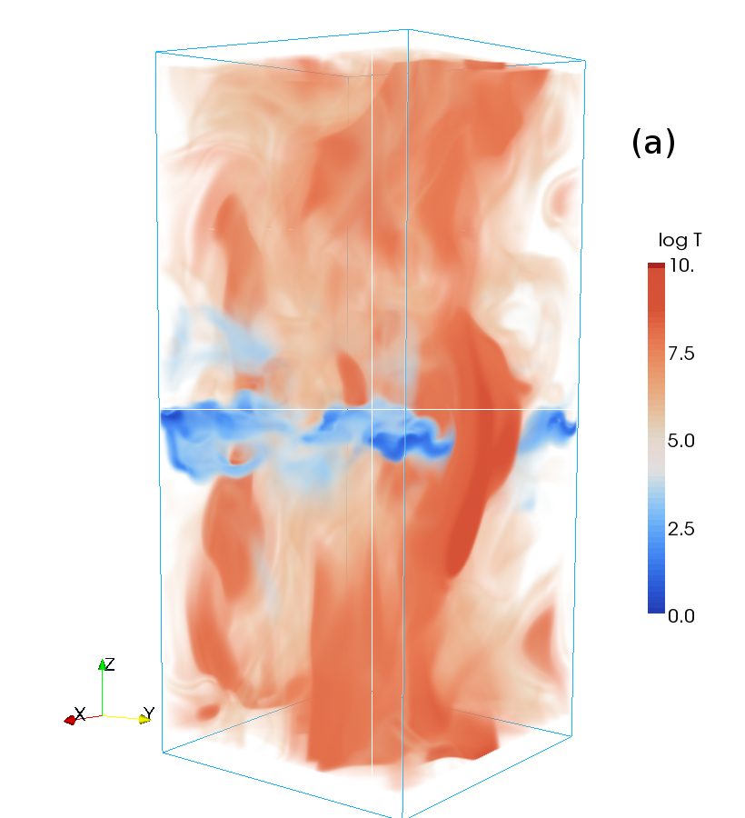
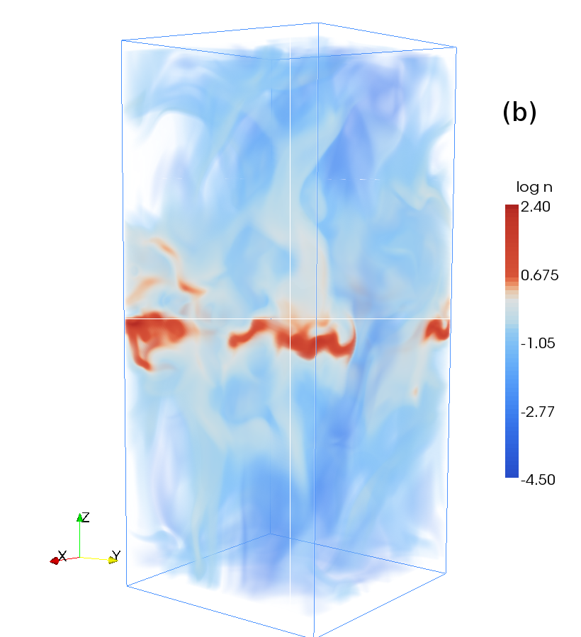
Figure 2 shows typical temperature and density distributions in this model at (i.e., after the restart from Model WSWb with reduced density). Supernova remnants appear as irregularly shaped regions of hot, dilute gas. A hot bubble breaking through the cold gas layer extends from the mid-plane towards the lower boundary, visible as a vertically stretched region in the temperature snapshot near the -face. Another, smaller one can be seen below the mid-plane near the -face. Cold, dense structures are restricted to the mid-plane and occupy a small part of the volume. Very hot and cold regions exist in close proximity.
Horizontally averaged quantities are shown in Fig. 3 as functions of and time for Model WSWb at , and WSWa at later times, showing the effect of reducing the total mass of gas at the transition time. Average quantities may have limited physical significance because the multi-phase gas has an extremely wide range of velocities, temperatures and densities. For example, panel (b) shows that the average temperature near the mid-plane, , is, perhaps unexpectedly, generally higher than that at the larger heights. This is due to Type II SN remnants, which contain very hot gas with and are concentrated near the mid-plane; even though their total volume is small, they significantly affect the average temperature.
Nevertheless these help to illustrate some global properties of the multi-phase structure. Before the system settles into a quasi-stationary state at about , it undergoes a few large-scale transient oscillations involving quasi-periodic vertical motions. The period of approximately 100 Myr, is consistent with the breathing modes identified by Walters & Cox (2001) and attributed to oscillations in the gravity field. Gas falling from high altitude overshoots the midplane and thus oscillates around it. Turbulent and molecular viscosities dampen these modes. At later times, a systematic outflow develops with an average speed of about ; we note that the vertical velocity increases very rapidly near the mid-plane and varies much less at larger heights. The result of the reduction of gas density at is clearly visible, as it leads to higher mean temperatures and a stronger and more regular outflow, together with a less pronounced and more disturbed layer of cold gas.
4 The multi-phase structure

All models discussed here have a well-developed multi-phase structure apparently similar to that observed in the ISM. Since the ISM phases are not genuine, thermodynamically distinct phases (Vázquez-Semadeni, 2012, e.g.), their definition is tentative, with the typical temperatures of the cold, warm and hot phases usually adopted as , – and , respectively. However, the borderline temperatures (and even the number of distinct phases) can be model-dependent, and they are preferably determined by considering the results, rather than a priori. Inspection of the probability distribution of gas number density and temperature, displayed in Fig. 4, reveals three distinct concentrations at and . Thus, we can confirm that the gas structure in this model can be reasonably well described in terms of three distinct phases. Moreover, we can identify the boundaries between them as the temperatures corresponding to the minima of the joint probability distribution at about and .
The curves of constant cooling time, also shown in Fig. 4, suggest that the distinction between the warm and hot gas is due to the maximum of the cooling rate near (see also Fig. 1), whereas the cold, dense gas, mainly formed by compression (see below), closely follows the curve .


In Fig. 5, we show the probability distributions of gas number density, random velocity, Mach number, thermal and total pressures within each phase in Model WSWa. The overlap in the gas density distributions (Fig. 5a) is small (at the probability densities of order ). The ratios of the probability densities near the maximum for each phase (mode) are about 100; the modal densities, and , thus typify the hot, warm and cold gas respectively.
The velocity probability distributions in Fig 5b reveal a clear connection between the magnitude of the random velocity of gas and its temperature: the r.m.s. velocity in each phase scales with its speed of sound. This is confirmed by the Mach number distributions in Fig. 5c: both warm and hot phases are transonic with respect to their sound speeds. The cold gas is mostly supersonic, having speeds typically under . The double peak in the probability density for the cold gas velocity (Fig 5b) (and the corresponding extension of the Mach number distribution to ) is a robust feature, not dependent on the temperature boundary of the cold gas. This plausibly includes ballistic gas motion in the shells of SN remnants, as well as bulk motions of cold clouds at subsonic or transonic speed with respect to the ambient warm gas.
Probability densities of thermal pressure, shown in Fig. 5d, are notable for the relatively narrow spread: one order of magnitude, compared to a spread of six orders of magnitude in gas density. Moreover, the three phases have overlapping thermal pressure distributions, suggesting that the system is in a statistical thermal pressure balance. However, thermal pressure is not the only part of the total pressure in the gas, which here includes the turbulent pressure , where , defined in Eq. (6), is the mean fluctuation velocity. As shown in Fig. 13, total kinetic energy within the computational domain, associated with random flows, is about a third of the thermal pressure. Correspondingly, the total pressure distributions in Fig. 5e peaks at about (or ), for both the warm and hot gas. The cold gas appears somewhat overpressured, with the modal pressure at , and with some regions under pressure as high as . It becomes apparent (see the discussion of Fig 7, below) that this is due to both compression by transonic random flows and the vertical pressure gradient. All the cold gas occupies the higher pressure mid-plane, while the warm and hot gas distributions mainly include lower pressure regions away from the disc.
Cold, dense clouds are formed through radiative cooling facilitated by compression, which has more importance than in the other, hotter phases. The compression is, however, truncated at the grid scale of 4 pc, preventing the emergence of higher densities in excess of about .

| Phase | [] | [] |
|---|---|---|
| cold | ||
| warm () | ||
| warm () | ||
| warm (total) | ||
| hot () | ||
| hot () |
The probability distributions of gas density in Fig. 5a can be reasonably approximated by the lognormal distributions, of the form
| (13) |
The quality of the fits is illustrated in Fig. 6, using 500 data bins in the range ; the best-fit parameters are given in Table 4. Note that, in making these fits, we have subdivided the hot and warm gas into that near the mid-plane () and that at greater heights (); the former is located in the SN active region, strongly shocked with a broad range of density and pressure fluctuations, whereas the latter is predominantly the more diffuse and homogeneous gas in the halo. As can be seen in Fig. 6, the shape of the probability distribution of the warm gas (rather than the position of its maximum) does not var much with . Table 4, thus shows the parameters for the warm in the whole volume. The lognormal fits satisfy the Kolmogorov-Smirnov test at or above the 95% level of significance. For the hot gas fit the KS test fails for the total volume. So only the fits for the hot gas split by height are included in Table 4.


The probability densities of thermal and total pressure, displayed in Fig. 7, show that although the thermal pressure of the cold gas near the mid-plane is lower than in the other phases the total pressures are much closer to balance. The broad probability distribution of the cold gas density is consistent with multiple compressions in shocks. The hot and warm gas pressure distributions are also approximately lognormal. The gas at (dotted lines) appears to be in both thermal and total pressure balance.
In summary, we conclude that the system is close to the state of statistical pressure equilibrium: the total pressure has similar values and similar probability distributions in each phase. Joung et al. (2009) also conclude from their simulations that the gas is in both thermal and total pressure balance. This could be expected, since the only significant deviation from the statistical dynamic equilibrium of the system is the vertical outflow of the hot gas and entrained warm clouds (see Section 7).
5 The filling factor and fractional volume
5.1 Filling factors: basic ideas
The fractional volume of the ISM occupied by the phase is given by
| (14) |
where is the volume occupied by gas in the temperature range defining phase and is the total volume. How the gas is distributed within a particular phase is described by the phase filling factor
| (15) |
where the over bar denotes a phase average, i.e., an average only taken over the volume occupied by the phase . describes whether the gas density of a phase is homogeneous () or clumpy (). Both of these quantities are clearly important parameters of the ISM, allowing one to characterise, as a function of position, both the relative distribution of the phases and their internal structure. As discussed below, the phase filling factor is also directly related to the idea of an ensemble average, an important concept in the theory of random functions and so provides a useful connection between turbulence theory and the astrophysics of the ISM. Both and are easy to calculate in a simulated ISM by simply counting mesh-points.
In the real ISM, however, neither nor can be directly measured. Instead the volume filling factor can be derived (Reynolds, 1977; Kulkarni & Heiles, 1988; Reynolds, 1991),
| (16) |
for a given phase , where the angular brackets denote a volume average, i.e., taken over the total volume. 22 2 As with the density filling factors introduced here, filling factors of temperature and other variables can be defined similarly to Eqs. (15) and (16), for example , etc.
Most work in this area to-date has concentrated on the diffuse ionised gas (or warm ionised medium) since the emission measure of the free electrons and the dispersion measure of pulsars , allowing to be estimated along many lines-of-sight (Reynolds, 1977; Kulkarni & Heiles, 1988; Reynolds, 1991; Berkhuijsen et al., 2006; Hill et al., 2008; Gaensler et al., 2008, e.g.). It is useful to generalise the tools derived to interpret the properties of a single ISM phase for the case of the multiphase ISM, as this can help to avoid potential pitfalls when combining data from different sources with similar-sounding names (filling factor, filling fraction, fractional volume, etc.) but subtly different meanings. In particular, only under the very specific conditions explained below, do the volume filling factors of the different phases of the ISM sum to unity.
In terms of the volume occupied by phase ,
| (17) |
whilst
| (18) |
the final equality holding because outside the volume by definition. Since the two types of averages differ only in the volume over which they are averaged, they are related by the fractional volume:
| (19) |
and
| (20) |
Consequently, the volume filling factor and the phase filling factor are similarly related:
| (21) |
Thus the parameters of most interest, and , characterizing the fractional volume and the degree of homogeneity of a phase respectively, are related to the observable quantity by Eq. (21). This relation is only straightforward when the ISM phase can be assumed to be homogeneous or if one has additional statistical knowledge, such as the probability density function, of the phase. In the next sub-section we use two simple examples to illustrate how the ideas developed here can be applied to the real ISM; we then use them to develop a new interpretation of existing observational data and finally discuss how the properties of our simulated ISM compare to observations. But first a brief note about different methods of averaging is necessary.
5.1.1 Averaging methods for observations and theory
An important feature of the definition of the volume filling factor given by Eq. (15), is that the averaging involved is inconsistent with that used in theory of random functions. In the latter, the calculation of volume (or time) averages is usually complicated or impossible and, instead, ensemble averages (i.e. averages over the relevant probability distribution functions) are used; the ergodicity of the random functions is relied upon to ensure that the two averages are identical to each other (Monin & Yaglom, 2007; Tennekes & Lumley, 1972, Section 3.3 in). But the volume filling factors are not compatible with such a comparison, as they are based on averaging over the total volume, despite the fact that each phase occupies only a fraction of it. In contrast, the phase averaging used to derive is performed only over the volume of each phase, and so should correspond better to results from the theory of random functions.
5.2 Filling factors: applications
5.2.1 Assumption of homogeneous phases
The simplest way to interpret an observation of the volume filling factor is to assume that each ISM phase has a constant density. Consider Eqs. (14), (15) and (16) for an idealised two-phase system, where each phase is homogeneous. (These arguments can easily be generalised to an arbitrary number of homogeneous phases.) For example a set of discrete clouds of one phase, of constant density and temperature, embedded within the other phase, with different (but also constant) density and temperature. Let one phase have (constant) gas number density and occupy volume , and the other and , respectively. The total volume of the system is .
The volume-averaged density of each phase, as required for Eq. (16), is given by
| (22) |
where . Similarly, the volume average of the squared density is
| (23) |
The fractional volume of each phase can then be written as
| (24) |
with , and . The volume-averaged quantities satisfy and , with the density variance .
In contrast, the phase-averaged density of each phase, used to calculate the phase filling factor Eq. (15), is simply , and the phase average of the squared density is , so that the phase filling factor is , as must be the case for a homogeneous phase.
Thus for homogeneous phases, the volume filling factor and the fractional volume of each phase are identical to each other, , and both sum to unity when considering all phases; in contrast, the phase-averaged filling factor is unity for each phase, . If a given phase occupies the whole volume (i.e., we have a single-phase medium), then all three quantities are simply unity: .
Whilst an assumption of homogeneous phases may be justified for some ISM phases, perhaps in specific regions of the galactic disc, in the case of the simulated ISM discussed in this paper such an assumption would lead to significant underestimates of for all phases, by a factor of 2 for the cold and hot gas and by an order of magnitude for the warm gas.
5.2.2 Assumption of lognormal phases
For the more realistic case of an inhomogeneous ISM, where each phase consists of gas with a range of densities, the interpretation of requires additional knowledge about the statistical properties of a phase.
For electrons in the diffuse ionised gas Reynolds (1977) derived the correction factor , where is the average density of electron clouds and the density variance within clouds, to allow for clumpiness in the electron distribution when calculating the fraction of the total path length occupied by the clouds. More generally, the probability distribution function of the gas in a phase allows to be calculated directly, as we now illustrate for the case of the lognormal PDFs identified in Section 4.
For a lognormal distribution , Eq. (13), the mean and mean-square densities are given by the following phase (‘ensemble’) averages:
| (25) |
where is the density variance around the mean , so that
| (26) |
So the phase filling factor only for a homogeneous density distribution, (or equivalently, ). This makes it clear that this filling factor, defined in terms of the phase average, is quite distinct from the fractional volume, , but rather quantifies the degree of homogeneity of the gas distribution within a given phase. Both describe distinct characteristics of the multi-phase ISM, and, if properly interpreted, can yield rich information about the structure of the ISM.
In the case of the simulated ISM, using the lognormal description of the phases given in Table 4 gives a reasonable agreement between the actual and estimated and for all phases, with the biggest discrepancy being an underestimate of against a true value of .
5.2.3 Application to observations
Observations can be used to estimate the volume-averaged filling factor , defined in Eq. (16), for a given ISM phase. On its own, this quantity is of limited value in understanding how the phases of the ISM are distributed: of more use are the fractional volume occupied by the phase , defined in Eq. (14), and its degree of homogeneity which is quantified by , defined by Eq. (15). Knowing and , follows via Eq. (21):
| (27) |
This formula is exact, but its applicability in practise is limited if is unknown. However can be deduced from the probability distribution of : for example if the the density probability distribution of the phase can be approximated by the lognormal, as is expected for a turbulent compressible gas (Vázquez-Semadeni & Garcia, 2001; Elmegreen & Scalo, 2004), then can be estimated from Eq. (26).
To illustrate how these quantities may be related, let us consider some observations reported for the diffuse ionised gas (the general approach suggested can be applied to any observable or computed quantity). Berkhuijsen et al. (2006) and Berkhuijsen & Müller (2008) estimated for the diffuse ionised gas (DIG) in the Milky Way using dispersion measures of pulsars and emission measure maps. In particular, Berkhuijsen et al. (2006) obtain towards , and Berkhuijsen & Müller (2008) find the smaller value for a selection of pulsars that are closer to the Sun than the sample of Berkhuijsen et al. (2006). On the other hand, Berkhuijsen & Fletcher (2008); Berkhuijsen & Fletcher (2012) used the same data for pulsars with known distances to derive PDFs of the distribution of average DIG cloud densities which are well described by a lognormal distribution; the fitted lognormals have (Berkhuijsen & Fletcher, 2012, Table 1 in ). Using Eqs. (26) and (27), this implies that the fractional volume of DIG with allowance for its inhomogeneity is about
In other words the combination of and from these results imply that the DIG is approximately homogeneous. This value of is in good agreement with the earlier estimates of Reynolds (1977) and Reynolds (1991) who obtained and close to that of Hill et al. (2008) who obtained for a vertically stratified ISM, by comparing observed emission and dispersion measures to simulations of isothermal MHD turbulence.
Volume density PDFs derived from observations are still rare. However, PDFs of the column density (and similar observables such as emission measure and dispersion measure) are more easily derived. The applicability of the method outlined in this Section, of deriving the fractional volume occupied by different ISM phases from the (observable) volume filling factor and the PDF of the density distribution, would improve as the relation between the statistical parameters of volume and column density distributions becomes better understood.
5.2.4 Simulation results


The filling factors and fractional volumes from Equations (14), (16) and (15) have been computed for the phases identified in Section 4 for the reference model WSWa and presented in Fig. 8. Volumes are considered as discrete horizontal slices. To isolate the -dependence we averaged over slices of single cell thickness (-thick).
The hot gas (Fig. 8c) accounts for about 70% of the volume at and about 40% near the mid-plane. The local maximum of the fractional volume of the hot gas at is due to the highest concentration of SN remnants there, filled with the very hot gas. Regarding its contribution to integrated gas parameters, it should perhaps be considered as a separate phase.
At the warm gas accounts for over 50% of the volume. The cold gas occupies a negligible volume, even in the mid-plane where it is concentrated. It is, however, quite homogeneous at low compared to the warm and hot phases, which only become relatively homogeneous at (Fig. 8a).
6 The correlation scale of the random flows

We have estimated the correlation length of the random velocity at a single time step of the model WSWa, by calculating the second-order structure functions of the velocity components , and , where
| (28) |
with the position in the -plane and a horizontal offset. We did not include offsets in the -direction and aggregated the squared differences by only. Since the flow is expected to be statistically homogeneous horizontally, while the correlation length is expected to vary with . A future paper will analyse in more detail the three-dimensional properties of the random flows, including its anisotropy and dependence on height. We measured for five different heights, , and , averaging over six adjacent slices in the -plane at each position, corresponding to a layer thickness of 20 pc. The averaging took advantage of the periodic boundaries in and ; for simplicity we chose a simulation snapshot at a time for which the offset in the -boundary, due to the shearing boundary condition, was zero. The structure function for the mid-plane () is shown in Fig. 9.
The correlation scale can be estimated from the form of the structure function since velocities are uncorrelated if exceeds the correlation length , so that becomes independent of , for . Precisely which value of should be chosen to estimate in a finite domain is not always clear; for example, the structure function of in Fig. 9 allows one to make a case for either the value at which is maximum or the value at the greatest . Alternatively, and more conveniently, one can estimate via the autocorrelation function , related to by
| (29) |
In terms of the autocorrelation function, the correlation scale is defined as
| (30) |
and this provides a more robust method of deriving in a finite domain. Of course, the domain must be large enough to make negligible at scales of the order of the domain size; this is a nontrivial requirement, since even an exponentially weak tail can make a finite contribution to . In our estimates we are, of course, limited to the range of within our computational domain, so that the upper limit in the integral of Eq. (30) is equal to , the horizontal box size.


Figure 10 shows for five different heights in the disc, where was taken to correspond to the absolute maximum of the structure function, , from Eq. (29) at each height.
The autocorrelation function of the vertical velocity varies with more strongly than, and differently from, the autocorrelation functions of the horizontal velocity components; it broadens as increases, meaning that the vertical velocity is correlated over progressively greater horizontal distances. Already at , is coherent across a significant horizontal cross-section of the domain, and at so is . An obvious explanation for this behaviour is the expansion of the hot gas streaming away from the mid-plane, which thus occupies a progressively larger part of the volume as it flows towards the halo.
| [] | [] | ||||||
|---|---|---|---|---|---|---|---|
Table 5 shows the rms velocities derived from the structure functions for each component of the velocity at each height, and the correlation lengths obtained from the autocorrelation functions. Note that these are obtained without separation into phases. The uncertainties in due to the choices of local maxima in are less than . However, these can produce quite large systematic uncertainties in , as small changes in can lead to becoming negative in some range of (i.e. a weak anti-correlation), and this can significantly alter the value of the integral in Eq. (30). Such an anti-correlation at moderate values of is natural for incompressible flows; the choice of and the estimate of are thus not straightforward. Other choices of in Fig. 9 can lead to a reduction in by as much as . Better statistics, derived from data cubes for a number of different time-steps, will allow for a more thorough exploration of the uncertainties, but we defer this analysis to a later paper.

The rms velocities given in Table 5 are compatible with the global values of and for the reference Model WSWa shown in Table 3. The increase in the rms value of with height, from about at to about at , reflects the systematic net outflow with a speed increasing with . There is also an apparent marginal tendency for the rms values of and to decrease with increasing distance from the mid-plane.
The correlation scale of the random flow is very close to in the mid-plane, and we have adopted this value for elsewhere in the paper. This estimate is in good agreement with the hydrodynamic ISM simulations of Joung & Mac Low (2006), who found that most kinetic energy is contained by fluctuations with a wavelength (i.e. in our notation) of . In the MHD simulations of Korpi et al. (1999), for the warm gas was at all heights, but that of the hot gas increased from in the mid-plane to at . de Avillez & Breitschwerdt (2007) found on average, with strong fluctuations in time. As in Korpi et al. (1999), there is a weak tendency for of the horizontal velocity components to increase with in our simulations, but this tendency remains tentative, and must be examined more carefully to confirm its robustness.
7 Gas flow to and from the mid-plane
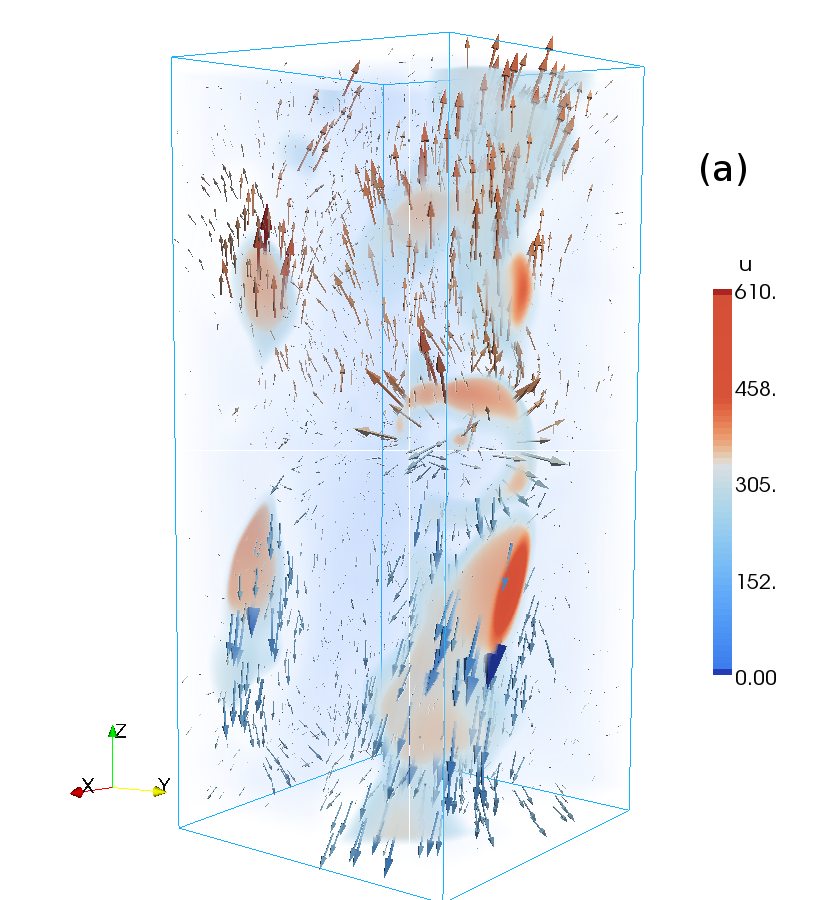
Figure 11 illustrates the 3D structure of the perturbation velocity field for the reference Model WSWa. Shades of red show the regions of high speed, whereas regions moving at speeds below about are transparent to aid visualisation. Velocity vectors are shown in panel (a) using arrows, with size indicating the speed, and colour indicating the sign of the -component of the velocity (indicating preferential outflow from the mid-plane). Red patches are indicative of recent SN explosions, and there is a strongly divergent flow close to the middle of the -face. In addition, stream lines in panel (b) display the presence of considerable small scale vortical flow near the mid-plane.


The mean vertical flow is dominated by the high velocity hot gas, so it is instructive to consider the velocity structure of each phase separately. Figure 12 shows the probability distributions as functions of in the -plane from 11 snapshots of Model WSWa, separately for the cold (a), warm (b) and hot gas (c). The cold gas is mainly restricted to and its vertical velocity varies within . As indicated by the red dashed curve in Panel (a), on average, the cold gas moves towards the mid-plane, presumably after cooling at larger heights. The warm gas is involved in a weak net vertical outflow above , of order . This might be an entrained flow within the hot gas. However, due to its skewed distribution, the modal flow and thus mass transfer is typically towards the mid-plane. The hot gas has large net outflow speeds, accelerating to about within , but with small amounts of inward flowing gas at all heights. The mean hot gas outflow speed increases at an approximately constant rate to somewhat over within of the mid-plane, and then decreases with further distance from the mid-plane, at a rate that gradually decreases with height for . This is below the escape velocity in the gravitational potential adopted. The structure of the velocity field shall be investigated further elsewhere.
8 Sensitivity to model parameters


8.1 The cooling function


We consider two models, RBN and WSWb, with parameters given in Table 3, to assess the effects of the specific choice of the cooling function. Apart from different parameterizations of the radiative cooling, the two models share identical parameters, except the value of was slightly higher in Model RBN, because of the sensitivity of the initial conditions to the cooling function (Section 2.4.4).
The volume-averaged thermal and kinetic energy densities, the latter excluding the imposed shear flow , are shown in Fig. 13 as functions of time. The averages for each are shown in Columns (11) and (12), respectively of Table 3, using the appropriate steady state time intervals given in Column (4). Models reach a statistical steady-state, with mild fluctuations around a well defined mean value, very soon (within 60 Myr of the start of the simulations). The effect of the cooling function is evident: both the thermal and kinetic energies in Model RBN are about 60% of those in Model WSWb. This is understandable as Model RBN has a stronger cooling rate than Model WSWb, only dropping below the WSW rate in the range (see Fig. 1). Interestingly, both models are similar in that the thermal energy is about times the kinetic energy.
These results are also remarkably consistent with results by Balsara et al. (2004, their Fig. 6) and Gressel (2008, Fig. 3.1). Gressel (2008) applies WSW cooling and has a model very similar to Model WSWa, with half the resolution and . He reports average energy densities of 24 and 10 (thermal and kinetic, respectively) with SN rate , comparable to 30 and 13 obtained here for Model WSWa.
Balsara et al. (2004) simulate an unstratified cubic region in size, driven at SN rates of 8, 12 and 40 times the Galactic rate, with resolution more than double that of Model WSWa. For SN rates and , they obtain average thermal energy densities of about 225 and 160, and average kinetic energy densities of 95 and 60, respectively (derived from their energy totals divided by the volume).
To allow comparison with our models, where the SNe energy injection rate is , if we divide their energy densities by 12 and 8, respectively, the energy densities would be 19 and 20 (thermal), and 8 and 7.5 (kinetic). These are slightly lower than our results with RBN cooling (25 and 9 ), but are below those with WSW (30 and 13 for WSWa, as given above). Balsara et al. (2004) used an alternative cooling function (Raymond & Smith, 1977), so allowing for some additional uncertainty over the net radiative energy losses, the results appear remarkably consistent.
While cooling and resolution may marginally affect the magnitudes, it appears that thermal energy density may consistently be expected to be about times the kinetic energy density, in these models. It also appears, by comparing the stratified and unstratified models, that the ratio of thermal to kinetic energy is not strongly dependent on height over the range included in our model.
The two models are further compared in Fig. 14, where we show probability distributions for the gas density, temperature and thermal pressure. With both cooling functions, the most probable gas number density is around ; the most probable temperatures are also similar, at around . With the RBN cooling function, the density range extends to smaller densities than with WSWb; and yet the temperature range for WSWb extends to lower values than for RBN. It is evident that the isobarically unstable part of the WSW cooling function does significantly reduce the amount of gas at 313–6102 K (the temperature range corresponding to the thermally unstable regime of the WSW cooling), and increase the amount of gas below 100 K. However this is not associated with higher densities than when using the RBN cooling function. This may indicate that multiple compressions, rather than thermal instability, dominate the formation of dense clouds.
The most probable thermal pressure is lower in Model RBN than in WSWb, consistent with the lower thermal energy content of the former.
The probability distributions of various quantities, shown in Fig. 15, confirm the clear phase separation in terms of gas density and perturbation velocity. Here we used the same borderline temperatures for individual phases as for Model WSWa (Fig. 5). Despite minor differences between the corresponding panels in Figs. 5 and 15, the peaks in the gas density probability distributions are close to and in all models. Given the extra cooling of hot gas and reduced cooling of cold gas with the RBN cooling function, more of the gas resides in the warm phase in Model RBN. The thermal pressure distribution in the hot gas reveals the two ‘types’ (see the end of section 4), which are mostly found within (high pressure hot gas within SN remnants) and outside this layer (diffuse, lower pressure hot gas). The probability distribution for the Mach number in the warm gas extends to higher values with the RBN cooling function, perhaps because more shocks reside in the more widespread warm gas, at the expense of the cold phase. It is useful to remember that, although each distribution is normalised to unit underlying area, the fractional volume of the warm gas is about a hundred times that of the cold phase.
The probability distributions of density and pressure in without preliminary separation into phases, presented in Fig. 14 do not show clear separations into phases (Joung & Mac Low, 2006; de Avillez & Breitschwerdt, 2004, cf. e.g. ), such that division into three phases would arguably only be conventional, if based on these alone. The probability distributions near the mid-plane, Fig. 14, exhibit a marginally better phase separation for the gas density (smaller frames in Fig. 14) (see also Korpi et al., 1999; Hill et al., 2012, their Figs. 1; and 6, respectively). However our analysis in terms of phase-wise PDFs confirms that the trimodal structure evident in the temperature distribution (Fig. 14b) has a complementary structure in the gas density.
Stratification of the thermal structure is clarified in Fig. 16, where we introduce narrower temperature bands specified in Table 6. The fractional volume of gas in each temperature range at a height is given by
| (31) |
similarly to Eq. (14), where is the number of grid points in the temperature range , with and given in Table 6, and is the total number of grid points at that height.
The fractional volumes in Column (13) of Table 3 show that near the mid-plane cold gas forms in similar abundances, independent of the cooling function. However, much less hot gas is achieved for Model RBN. Figure 16 also helps show how the thermal gas structure depends on the cooling function. Model WSWb, panel (b), has significantly more very cold gas () than RBN, panel (a), but slightly warmer cold gas () is more abundant in RBN. The warm and hot phases () have roughly similar distributions in both models, although Model RBN has less of both phases. Apart from relatively minor details, the effect of the form of the cooling function thus appears to be straightforward and predictable: stronger cooling means more cold gas and vice versa. What is less obvious, however, is that the very hot gas is more abundant near in Model RBN than in WSWb, indicating that the typical densities must be much lower. This, together with the greater abundance of cooler gas near the mid-plane, suggest that there is less stirring with RBN cooling.
Altogether, we conclude that the properties of the cold and warm phases are not strongly affected by the choice of the cooling function. The main effect is that the RBN cooling function produces less hot gas with significantly lower pressures. This can readily be understood, as this function provides significantly stronger cooling at .


8.2 The total gas mass
Models RBN and WSWb have about 17% more mass of gas than the reference Model WSWa, where we have removed that part of the gas mass which should be confined to molecular clouds unresolved in our simulations (as described in section 3). The difference is apparent in comparing Fig. 16b with Fig. 17b (or Fig. 17a). Higher gas mass causes the abundance of hot gas to reduce with height, contrary to observations, and to the behaviour of Model WSWa. Otherwise, the fractional volumes within of the mid-plane appear independent of the gas mass.


8.3 Numerical resolution


Models WSWa and WSWah differ only in their resolution, using 2 and 4 pc, respectively. Model WSWah is a continuation of the state of WSWa after 600 Myr of evolution.


The most obvious effect of increased resolution is the increase in the magnitude of the perturbed velocityand temperatures; in Model WSWa increasing to in Model WSWah (Table 3, Column 9) and from 150 to (Column 6). Both and the random velocity are increased by a similar factor of about 1.3. However, the thermal energy is reduced by a factor of 0.6 with the higher resolution, while kinetic energy remains about the same. This suggests that in the higher-resolution model, the higher velocities and temperatures are associated with lower gas densities.
The vertical distribution of the fractional volume in each temperature range (defined in Table 6) is shown in Fig. 17 for Model WSWah (panel a) for comparison with Model WSWa in (c). The fractional mass (b) is calculated similarly to Eq. (31) is
| (32) |
where is the mass of gas within temperature range at a given , and is the total gas mass at that height.
Note that the relative abundances of the various phases in these models might be affected by the unrealistically high thermal conductivity adopted. The coldest gas (black, solid), with , is largely confined within about of the mid-plane. Its fractional volume (Fig. 17a,c) is small even at the mid-plane, but it provides more than half of the gas mass at (Fig.17b). Gas in the next temperature range, (purple, dash-dotted), is similarly distributed in . Models WSWa and WSWah differ only in their resolution, using 2 and 4 pc, respectively. Model WSWah is a continuation of the state of WSWa after 600 Myr of evolution. With higher resolution the volume fraction of the coldest gas is significantly enhanced (Fig. 17c compared to a), but it is similarly distributed.
Gas in the range (dark blue, dashed) has a similar profile to the cold gas for both the fractional mass and the fractional volume, and this is insensitive to the model resolution. This is identified with the warm phase, but exists in the thermally unstable temperature range. It accounts for about 10% by volume and 20% by mass of the gas near the mid-plane, which is consistent with observational evidence. It is negligible away from the supernova active regions.
The two bands with (red, dotted and orange, dash-3dotted) behave similarly to each other (Fig. 17a,c), occupying similar fractional volumes for , and with increasing above this height (more rapidly for the hotter gas). In contrast the fractional masses (Fig. 17b) in these temperature bands are negligible for , and increase above this height (less rapidly for the hotter gas). The temperature band (green/black, dash-3dotted) is similarly distributed to the hotter gas (orange) in all profiles. It is however identified with the warm phase, indicating that this is mainly hot gas cooling, a transitional state, which accounts for a relatively small volume fraction of the warm gas and especially a small mass fraction. The dramatic effect of increased resolution (Fig. 17a compared to c) is the significant increase in the very hot gas (red, dotted), particularly displacing the hotter gases (orange and green) but also to some degree the bulk warm gas (blue, dashed). This reflects the reduced cooling due to the better density contrasts resolved, associating the hottest temperatures to the most diffuse gas.
The middle temperature range has a distinctive profile in both fractional volume and fractional mass, with minima near the mid-plane and maxima at about , being replaced as the dominant component by hotter gas above this height. The fractional volume and vertical distribution of this gas is quite insensitive to the resolution. The distribution of the warm gas (; blue, long-dashed) does not change much with increased resolution. However, the higher-resolution model has more of the cold phase (; black, solid and dash-dotted) and, especially, of the very hottest gas (; red, dotted), at the expense of the intermediate temperature ranges.
This can also be seen in the gas density and temperature probability distributions shown in Fig. 18(a), (b): increased resolution modestly increases the abundance of cold gas and significantly enhances the amount of very hot gas. The minima in the distributions (at density , and at temperatures and K) appear independent of resolution, suggesting that the phase separation is physical, rather than numerical. The distributions are most consistent in the thermally unstable range 313–6102 K. Higher resolution also reduces the minimum further about the unstable range above , as the highest temperature gas has lower losses to thermal conduction. The mean temperatures of the cold gas ( K) warm gas ( K) and the mean warm gas density () also appear to be independent of the resolution. However the natural log mean is about -8 for the hot gas, both within and without of the mid-plane (with larger standard deviation for the gas near the mid-plane). This compares with values of -6.97 and -5.78 in our model with resolution; i.e. a factor of about 1/3. This reflects the improved resolution of low density in the remnant interiors.
The density and temperature probability distributions for WSWa are similar to those obtained by Joung & Mac Low (2006, their Fig. 7), who used a similar cooling function, despite the difference in the numerical methods (adaptive mesh refinement down to in their case). With slightly different implementation of the cooling and heating processes, again with adaptive mesh refinement down to , de Avillez & Breitschwerdt (2004, their Fig. 3) found significantly more cool, dense gas. It is noteworthy that the maximum densities and lowest temperatures obtained in our study with a non-adaptive grid are of the same order of magnitude as those from AMR-models where the local resolution is up to three times higher. At our mean minimum temperature is , within the range – for 0.625– (de Avillez & Breitschwerdt, 2004, their Fig. 9). For mean maximum gas number, our is within their range –.
The vertical density profiles obtained under the different numerical resolutions are shown in Fig. 19a. Although the density distribution in Fig. 18a reveals higher density contrasts with increased resolution, there is little difference in the -profiles of the models. The mean gas number density at the mid-plane, — which with our course grid resolution excludes the contribution from Hii— is about : double the observation estimates summarised in Ferrière (2001). This might be expected in the absence of the magnetic and cosmic ray components of the ISM pressure, to help support the gas against the gravitational force.
However the vertical pressure distributions are consistent with the models of Boulares & Cox (1990, their Figs. 1 and 2), which include the weight of the ISM up to . The total pressure for the standard (high) resolution model is slightly above their estimate of about 1.9 for hot, turbulent gas. For the turbulent pressure alone we have falling to at and then remaining reasonably level. The pressures are generally slightly reduced with increased resolution, except for near the mid-plane. Small scales are better resolved, so the turbulent structures are a stronger component of the SN active region. These pressures are consistent with Boulares & Cox (1990), even though our model does not explicitly include the pressure contributions from the ISM above .
Comparing our thermal pressure distribution (Fig. 18c) with de Avillez & Breitschwerdt (2004, their Fig. 4a) and Joung et al. (2009, their Fig. 2), the three models peak at 3.16, 1.3 and , respectively. The latter models include and resolution up to 1.25 pc. Our data summarise the volume within , while the comparisons are within and respectively.
We conclude that the main effects of the increased resolution are confined to the very hot interiors and to the thin shells of SN remnants; the interiors become hotter and the SN shell shocks become thinner with increased resolution (see Appendix B). Simultaneously, the higher density of the shocked gas enhances cooling, producing more cold gas and reducing the total thermal energy. Otherwise, the overall structure of the diffuse gas is little affected: the probability distributions of thermal pressure are almost indistinguishable, with our standard resolution fractionally higher pressure (Fig. 18c).
We are satisfied that the numerical resolution of the reference model, , is sufficient to model the diffuse gas phases reliably. This choice of the working numerical resolution is further informed by tests involving the expansion of individual SN remnants (presented in Appendix B).
9 Discussion and conclusions


The multi-phase gas structure obtained in our simulations appears to be robust, with overall parameters relatively insensitive to the physical (Section 4) and numerical (Section 8.3) details, including the parameterizations of the radiative cooling tested here (Section 8.1). We have identified natural temperature boundaries of the major phases using the variation, with height above the mid-plane, of the fractional volume occupied by the gas in relatively narrow temperature ranges. This confirms that the system can be satisfactorily described in terms of just three major phases with temperature ranges , and . The most probable values of the variables we have explored (gas density, thermal and total pressure, perturbed velocity and Mach number) are practically independent of the cooling function chosen (Fig. 15). Moreover, this is true for the cold, warm and hot phases separately. A 3D rendering of a snapshot of the density distribution from the reference model WSWa is illustrated in Fig 20, showing the typical location and density composition of each phase separately.
A conspicuous contribution to various diagnostics — especially within of the mid-plane, where most of the SNe are localised — comes from the very hot gas within SN remnants. Regarding its contribution to integrated gas parameters, it should perhaps be considered as a separate phase.
The fractional volume occupied by each phase is a convenient diagnostic and an important physical parameter. We have clarified the relation between the fractional volume and various probabilistic measures of a random distribution of density (or of any other quantity), and established an exact relation between the fractional volume and various density averages obtainable observationally (in Section 5). This represents a significant improvement upon the assumption of locally homogeneous gas, the only analytical tool used to date in determinations of the fractional volumes of the phases.
The correlation scale of the random flows is obtained in Section 6, from the autocorrelation functions of the velocity components. Within of the mid-plane, the horizontal velocity components have a consistent correlation scale of about . In contrast, the scale of the vertical velocity (which has a systematic part due to the galactic outflow of hot gas) grows from about at the mid-plane to nearly at , and may do so further at larger heights (Korpi et al., 1999, cf.). This is due to the increase of the fractional volume of the hot gas with distance from the mid-plane. At most of the volume is occupied by the hot gas. As the interstellar gas flows out of the galactic disc into the halo, it must expand, and the scale of the expanding regions may be expected to become comparable to at . It would be helpful to obtain estimates of the horizontal correlation of the flow above , so that modelling of the galactic fountain might be adequately formulated.
We find clear indication of cold gas falling back towards the mid-plane at speeds of a few km/s, hot gas involved in vigorous outflow away from the mid-plane, and some warm gas entrained in this outflow (Section 7). The outflow speed of the hot gas increases up to within of the mid-plane and then slowly decreases. In contrast, the mean vertical velocity of the warm gas increases linearly with , up to towards the upper boundaries of our domain.
Given that probability densities for gas temperature and number density, calculated for individual phases, are clearly separated, the probability densities for both thermal and total pressure (the sum of thermal and turbulent) are not segregated at all. Despite its complex thermal and dynamical structure, the gas is in statistical pressure equilibrium. Since the SN-driven ISM is random in nature, both total and thermal pressure fluctuate strongly in both space and time (albeit with significantly smaller relative fluctuations than the gas density, temperature and perturbation velocity), so the pressure balance is also statistical in nature. These might appear to be obvious statements, since a statistical steady state (i.e., not involving systematic expansion or compression) must have such a pressure balance. Deviations from thermal pressure balance and observations of significant regions of gas within the classically forbidden thermally unstable range (300 – 6000), which is also evident in our probability distributions, may lead to conclusions of an ISM comprising a broad thermodynamic continuum in pressure disequilibrium (Vázquez-Semadeni, 2012, discussion on The controversy). The only systematic deviations from pressure balance are associated with the systematic outflow of the hot gas (leading to lower pressures), and with the compression of the cold gas by shocks and other converging flows (leading to somewhat increased pressures). Even this can be further reconciled if we allow for the global vertical pressure gradient (cf. Fig. 7). It is evident that phases are locally in total pressure equilibrium.
An important technical aspect of simulations of this kind is the minimum numerical resolution required to capture the basic physics of the multi-phase ISM. We have shown that is sufficient with the numerical methods employed here (Section 8.3). In addition to comparing results obtained for and with our own code, we have satisfied ourselves that our results are consistent with those obtained by other authors using adaptive mesh refinement with maximum resolutions of and .
As with all other simulations of the SN-driven ISM, we employ a host of numerical tools (such as shock-capturing diffusivity) to handle the extremely wide dynamical range ( and in terms of gas temperature and number density in our model) and widespread shocks characteristic of the multi-phase ISM driven by SNe. Their detailed description can be found in Section 2.4. We have carefully tested our numerical methods by reproducing, quite accurately, the Sedov–Taylor and snowplough analytical solutions for individual SN remnants (Appendix B).
The major elements of the ISM missing from the models presented here are magnetic fields and cosmic rays. Analysis of the structure of the velocity field and its interaction with the magnetic field, effects of rotation, shear and SN rates will be the subject of a future paper.
Acknowledgements
Part of this work was carried out under the programme HPC-EUROPA2 of the European Community (Project No. 228398) – Research Infrastructure Action of the FP7. We gratefully acknowledge the resources and support of the CSC-IT Center for Science Ltd., Finland, where the major part of the code adjustment and all of the final simulations were carried out. The contribution of Jyrki Hokkanen (CSC) to enhancing the graphical representation of the results is gratefully acknowledged. We used the UK MHD Computer Cluster in St Andrews, Scotland, for code development and testing. MJM is grateful to the Academy of Finland for support under Projects 218159 and 141017. The work of AF, GRS and AS has been supported by the Leverhulme Trust’s Research Grant RPG-097 and the STFC grant F003080. FAG has been supported by the EPSRC DTA grant to the Newcastle University. We thank Elly Berkhuijsen for insightful comments on filling factors and the anonymous referee for their conscientious and constructive contribution.
Appendix A Notation
| Symbol | Meaning |
|---|---|
| Adiabatic speed of sound | |
| Heat capacity at constant pressure | |
| Velocity autocorrelation function, Eq. (29) | |
| Advective derivative, Eq. (5) | |
| Velocity structure function, Eq. (28) | |
| Energy density, subscript thermal: ‘th’, kinetic: ‘kin’ | |
| Total energy injected into the ISM by a single SN | |
| Fractional mass of gas in phase , Eq. (32) | |
| Fractional volume occupied by the phase , Eq. (14) | |
| Vertical acceleration due to the Galactic gravity, Eq. (7) | |
| Scale height of the Type I SN distribution, Section 2.2 | |
| Scale height of the Type II SN distribution, Section 2.2 | |
| Boltzmann’s constant | |
| Thermal conductivity () | |
| Velocity correlation scale | |
| Proton mass | |
| Mach number | |
| Gas number density | |
| Gas density averaged within a given phase , Eq. (17) | |
| Gas density averaged over volume of phase , Eq. (18) | |
| Thermal pressure | |
| Total pressure (thermal plus turbulent) | |
| Probability density | |
| Characteristic radius of the SN energy injection site, Section 2.2 | |
| rms | Root-mean square |
| Specific entropy, | |
| Parameter of the lognormal probability distribution, Eq. (13) | |
| Velocity shear rate due to differential rotation | |
| SN | Supernova (also as a subscript) |
| Gas temperature | |
| Total volume of a region in Section 5.1 | |
| Volume occupied by an ISM phase labelled , Section 5.1 | |
| Velocity perturbation: deviation of the gas velocity from the background rotational flow | |
| Random velocity, p. 2.1 | |
| Large-scale shear flow (differential rotation), p. 2.1 | |
| W | Rate of strain tensor, Eq. (4) |
| Specific rate of photoelectric heating, | |
| Numerical mesh separation (resolution of a simulation) | |
| Shock-capturing viscosity | |
| Shock-capturing thermal diffusivity | |
| Radiative cooling rate, | |
| Molecular weight | |
| Parameter of the lognormal probability distribution, Eq. (13) | |
| Kinematic viscosity | |
| Type I SN rate per unit surface area, Section 2.2 | |
| Type II SN rate per unit surface area, Section 2.2 | |
| Angular velocity of the Galactic rotation | |
| Phase filling factor within the ISM phase , Eq. (15) | |
| Volume filling factor of the ISM phase , Eq. (16) | |
| Rate of mass injection, per unit volume, by SNe, Section 2.2 | |
| Gas density | |
| Rate of energy injection by SNe (per unit volume), as kinetic energy in Eq. (2) and as thermal energy in Eq. (3), see Section 2.2 | |
| Variance of ISM phase , Section 5 | |
| Radiative cooling time | |
| Gravitational potential | |
| Thermal diffusivity |
Table 7 contains most of the symbols used in the text and their explanation, arranged alphabetically.
Appendix B Evolution of an individual supernova remnant
The thermal and kinetic energy supplied by SNe drives, directly or indirectly, all the processes discussed in this paper. It is therefore crucial that the model captures correctly the energy conversion in the SN remnants and its transformation into the thermal and kinetic energies of the interstellar gas. As discussed in Section 2.2, the size of the region where the SN energy is injected corresponds to the adiabatic (Sedov–Taylor) or the snowplough stage. Given the multitude of artificial numerical effects required to model the extreme conditions in the multi-phase ISM, it is important to verify that the basic physical effects are not affected, while sufficient numerical control of strong shocks, rapid radiative cooling, supersonic flows, etc., is properly ensured. Another important parameter to be chosen is the numerical resolution.
Before starting the simulations of the multi-phase ISM reported in this paper, we have carefully confirmed that the model can reproduce, to sufficient accuracy, the known realistic analytical solutions for the late stages of SN remnant expansion, until merger with the ISM. The minimum numerical resolution required to achieve this in our model is . In this Appendix, we consider a single SN remnant, initialised as described in Section 2.2, that expands into a homogeneous environment. All the numerical elements of the model are in place, but here we use periodic boundary conditions in all dimensions.
The parameters and are as applied in Model WSWa for , but reduced here proportionally for and . The constant used in Eq. (10) to suppress cooling around shocks is unchanged. This may allow excess cooling at higher resolution, evident in the slightly reduced radii in Fig. 21. For Model WSWah, and were just as in Model WSWa; for future reference, they should be appropriately adjusted, as should , to better optimise higher resolution performance.
B.1 The adiabatic and snowplough stages


The Sedov–Taylor solution,
| (33) |
is accurately reproduced with our code at the resolution or higher. Here is the remnant radius, the explosion energy, the ambient gas density, and for (Ostriker & McKee, 1988).
Modelling even a single remnant becomes more challenging when radiative cooling becomes important. Here we compare numerical results with two analytic solutions for an SN remnant expanding into a perfect, homogeneous, monatomic gas at rest. The standard momentum-conserving snowplough solution for a radiative SN remnant has the form
| (34) |
where is the radius of the SN remnant at the time of the transition from the adiabatic stage, and is the shell expansion speed at . The transition time is determined by Woltjer (1972) as that when half of the SN energy is lost to radiation; this happens when
| (35) |
the transitional expansion speed thus depends very weakly on parameters.
Cioffi et al. (1998) obtained numerical and analytical solutions for an expanding SN remnant with special attention to the transition from the Sedov–Taylor stage to the radiative stage. These authors adjusted an analytical solution for the pressure-driven snowplough stage to fit their numerical results to an accuracy of within 2% and 5% in terms of and , respectively. (Their numerical resolution was in the interstellar gas and within ejecta.) They thus obtained
| (36) |
where the subscript denotes the radius and time for the transition to the pressure driven stage. The estimated time of this transition is
For ambient densities of , this yields transition times and shell radii , respectively, with speed
This continues into the momentum driven stage with
| (37) |
where subscript denotes the radius and time for this second transition,
where is the initial velocity of the ejecta. For each , the transitions occur at , and , respectively. The shell momentum in the latter solution tends to a constant, and the solution thus converges with the momentum-conserving snowplough (34); but, depending on the ambient density, the expansion may become subsonic and the remnant merge with the ISM before Eq. (34) becomes applicable.
We compare our results with the momentum-conserving snowplough solution and those of Cioffi et al. in Fig. 21, testing our model with numerical resolutions , 2 and 4 pc for the ambient gas densities . Shown in Fig. 21 are a linear plot of the remnant radius versus time to check if its magnitude is accurately reproduced, a double logarithmic plot of to confirm that the scaling is right, and variation of the expansion speed with time to help assess more delicate properties of the solution. We are satisfied to obtain good agreement with the analytical results for all the resolutions investigated when the ambient gas number density is below . For , the remnant radius is accurate to within about 3% for and underestimated by up to 6% for . At higher numerical resolutions, the remnant radius is underestimated by up to 7% and 11% for and , respectively. For , excellent agreement is obtained for the higher resolutions, and ; simulations with overestimate the remnant radius by about 20–25% in terms of and at . We emphasize that a typical SN explosion site in the models described in the main part of the paper has an ambient density so that , or produce a satisfactory fit to the results, despite the much finer resolution of the simulations, of Cioffi et al.
The higher than expected expansion speeds into dense gas can be explained by the artificial suppression of the radiative cooling within and near to the shock front as described by Eq. (10). Our model reproduces the low density explosions more accurately because the shell density is lower, and radiative cooling is therefore less important.


B.2 The structure of the SN remnant
Cuts through the simulated SN remnant are shown in Fig. 22 for gas density, temperature and velocity, obtained for resolution and with ambient density . In the temperature and velocity panels, we also include the profile of the shock viscosity from Eq. (9) (black dotted line), scaled to fit each plot. The temperature panels also show where net cooling is applied to the remnant, from Eq.(3) (blue dashed line), while the velocity panels also show the ambient sound speed (pink dashed lines). The top panel depicts the initial distributions, at , with which the mass of and each of thermal and kinetic energy are injected. The other panels are for and 1.02 after the start of the evolution, from top to bottom, respectively; the actual simulation continued to , when the remnant radius reached .
The position of the peak of the density profile is used to determine the shell radius shown in Fig. 21. The Rankine–Hugoniot jump conditions are not very well satisfied with the numerical parameters used here. This is due to our numerical setup, essentially designed to control the shocks by spreading them sufficiently to be numerically resolvable in production runs that contain many interacting shocks and colliding SN shells. Better shock front profiles have been obtained with other choices of parameters and cooling control, and with better resolution. The density and temperature contrasts across the shock fronts are reduced by the shock smoothing, which inhibits the peak density and enhances gas density behind the shocks. In an isolated remnant, the peak gas number density does not exceed , but in the full ISM simulation we obtain densities in excess of , as a result of interacting remnants and highly supersonic flows.
The interior of the SN remnant, if more dense due to numerical smoothing about the shock profile, would cool unrealistically rapidly, so that the SN energy would be lost to radiation rather than agitate the ambient ISM. The centre panels in Fig. 21 clarify how the cooling suppression described in Eq. (10) reduces the cooling rate in the relatively homogeneous interior of the remnant, while still allowing rapid cooling in the dense shell where the gradient of the shock viscosity is small. It is evident from the temperature cuts that the remnant still contains substantial amounts of hot gas when its radius reaches 100 pc, so it would be merging with the ISM in the full simulation.
The panels in the right column of Fig. 21 demonstrate that the interior gas velocity can be more than twice the shell speed. Due to the high interior temperature, this flow is subsonic, while the remnant shell expands supersonically with respect to its ambient sound speed. The enhanced viscosity in the hotter interior (with viscosity proportional to the sound speed; see Section 2.4) inhibits numerical instabilities that could arise from the high velocities. In fact, accurate modelling of the SN interiors is not essential in the present context (where we are mainly interested in a realistic description the multi-phase ISM), as long as the interaction of the remnant with the ambient gas is well described, in terms of the energy conversion and transfer to the ISM, the scales and energy of turbulence, and the properties of the hot gas.
Appendix C Boundary conditions and numerical control of advection and diffusion
C.1 Top and bottom boundaries
Unlike the horizontal boundaries of the computational domain, where periodic or sliding-periodic boundary conditions are adequate (within the constraints of the shearing box approximation), the boundary conditions at the top and bottom of the domain are more demanding. The vertical size of the galactic halo is of order of 10 kpc, and nontrivial physical processes occur even at that height, especially when galactic wind and cosmic ray escape are important. As explained in Section 2.4, we do not attempt to model the full extent of the halo here. Therefore, it is important to formulate boundary conditions at the top and bottom of the domain that admit the flow of matter and energy, while minimising any associated artifacts that might affect the interior.
Stress-free, open vertical boundaries would seem to be the most appropriate, requiring that the horizontal stresses vanish, while gas density, entropy and vertical velocity have constant first derivatives on the top and bottom boundaries. These are implemented numerically using ‘ghost’ zones; i.e., three outer grid planes that allow derivatives at the boundary to be calculated in the same way as at interior grid points. The interior values of the variables are used to specify their ghost zone values. When a sharp structure approaches the boundary, the strong gradients are therefore extrapolated into the ghost zones. This artificially enhances the prominence of such a structure, and may cause the code to crash. Here we describe how we have modified these boundary conditions to ensure the numerical stability of our model.
To prevent artificial mass sources in the ghost zones, we impose a weak negative gradient of gas density in the ghost zones. Thus, the density values are extrapolated to the ghost zones from the boundary point as
for all values of the horizontal coordinates and , where the boundary surfaces are at , and the ghost zones are at with . The upper (lower) sign is used at the top (bottom) boundary. This ensures that gas density gradually declines in the ghost zones.
To prevent a similar artificial enhancement of temperature spikes in the ghost zones, gas temperature there is kept equal to its value at the boundary,
so that temperature is still free to fluctuate in response to the interior processes. This prescription is implemented in terms of entropy, given the density variation described above.
Likewise, the vertical velocity in the ghost zones is kept equal to its boundary value if the latter is directed outwards,
However, when gas cools rapidly near the boundary, pressure can decrease and gas would flow inwards away from the boundary. To avoid suppressing inward flows, where we use the following: if , we set
otherwise, we set
In both cases, in the two outer ghost zones (), we set
so that the inward velocity in the ghost zones is always smaller than its boundary value. This permits gas flow across the boundary in both directions, but ensures that the flow is dominated by the interior dynamics, rather than by anything happening in the ghost zones.
The Pencil code is non-conservative, so that gas mass is not necessarily conserved; this can be a problem due to extreme density gradients developing with widespread strong shocks. Solving Eq. (1) for , rather than , solves this problem for the snowplough test cases described in Appendix B.1, with mass then being conserved within machine accuracy. However for the full model, once the ISM becomes highly turbulent, there remains some numerical mass loss. A comparison of mass loss through the vertical boundaries to the total mass loss in the volume indicates that numerical dissipation accounts for per . The rate of physical loss, from the net vertical outflow, was of order per .
C.2 Time step control
To achieve numerical stability with the explicit time stepping used, the CFL conditions have to be amply satisfied. For example, for advection terms, the numerical time step should be selected such that
where is the speed of sound, is the amplitude of the perturbed velocity, i.e., the deviation from the imposed azimuthal shear flow , and is a dimensionless number, determined empirically, which often must be significantly smaller than unity. Apart from the velocity field, other variables also affect the maximum time step, e.g., those associated with diffusion, cooling and heating, so that the following inequalities also have to be satisfied:
where and are further empirical constants and
We use and . The latter, more stringent constraint has a surprisingly small impact on the typical time step, but a large positive effect on the numerical accuracy. Whilst the time step may occasionally decrease to below 0.1 or 0.01 years following an SN explosion, the typical time step is more than 100 years.
C.3 Minimum diffusivity
Numerical stability also requires that the Reynolds and Péclet numbers defined at the resolution length , as well as the Field length, are sufficiently small. These mesh Péclet and Reynolds numbers are defined as
| (38) |
where is the maximum perturbed velocity and is the mesh length. For stability these must not exceed some value, typically between 1 and 10. Note that the Reynolds and Péclet numbers characterizing the flow are 25 times larger, since is replaced by as the relevant turbulent length scale in the non-mesh quantities.
In numerical modelling of systems with weak diffusivity, and are usually set constant, close to the smallest value consistent with the numerical stability requirements. This level strongly depends on the maximum velocity, and hence is related to the local sound speed, which can exceed in our model. To avoid unnecessarily strong diffusion and heat conduction in the cold and warm phases, we scale the corresponding diffusivity with gas temperature, as . As a result, the diffusive smoothing is strongest in the hot phase (where it is most required). This may cause reduced velocity and temperature inhomogeneities within the hot gas, and may also reduce the temperature difference between the hot gas and the cooler phases.
The effect of thermal instability is controlled by the Field length,
where we have neglected any heating. To avoid unresolved density and temperature structures produced by thermal instability, we require that , and so the minimum value of the thermal conductivity follows as
where is the minimum cooling time, and is the relevant exponent from the cooling function (e.g. as in Table 1 for WSW cooling). In the single remnant simulations of Appendix B, . In the full ISM simulations, minimum cooling times as low as were encountered. has maxima corresponding to for . All of these, except for that at , result in at , so are satisfied by default for any sufficiently high to satisfy the requirement. For , at we have . Thus if cooling times as short as 0.05 Myr were to occur in the cold gas, we would have , and would be marginally under-resolved. Our analysis of the combined distribution of density and temperature, however, indicates that cooling times this short occur exclusively in the warm gas.
With , as adopted in Section 2.4, then is near the limit of numerical stability. (We discuss our choice of thermal diffusivity further in Appendix D.) As a result, the code occasionally crashed (notably when hot gas was particularly abundant), and had to be restarted. When restarting, the position or timing of the next SN explosion was modified, so that the particularly troublesome SN that caused the problem was avoided. In extreme cases, it was necessary to increase temporarily (for only a few hundred time steps), to reduce the value of during the period most prone to instability, before the model could be continued with the normal parameter values.
Appendix D Thermal instability
One of the two cooling functions employed in this paper, WSW, supports isobaric thermal instability in the temperature range where . (Otherwise, for the RBN cooling function or outside this temperature range for WSW cooling, we have or , so the gas is either thermally stable or has no unstable equilibrium.)
Under realistic conditions of the ISM, thermal instability can produce very small, dense gas clouds which cannot be captured with the resolution used here. Although the efficiency of thermal instability is questionable in the turbulent, magnetized ISM, where thermal pressure is just a part of the total pressure (Vázquez-Semadeni et al., 2000; Mac Low & Klessen, 2004, and references therein), we prefer to suppress this instability in the model. However, we do that not by modifying the cooling function, but rather by enhancing thermal diffusivity so as to avoid the growth of perturbations at wavelengths too short to be resolved by our grid.
Following Field (1965), we introduce the characteristic wave numbers
where is the gas constant, and the derivatives and are calculated for constant and , respectively. The values of temperature and density in these equations, and , are those at thermal equilibrium, with . Isothermal and isochoric perturbations have the characteristic wave numbers and , respectively, whereas thermal conductivity is characterised by .
The control parameter of the instability is .
The instability is suppressed by heat conduction, with the largest unstable wave numbers given by (Field, 1965)
| (39) | ||||
| (40) |
for the condensation and wave modes, respectively, whereas the most unstable wave numbers are
| (41) | ||||
| (42) |
| [] | [pc] | [pc] | [pc] | [pc] | [pc] | ||
|---|---|---|---|---|---|---|---|
| 313 | 4.97 | 1.91 | 2 | 5 | 5 | 2 | 4 |
| 4000 | 1.20 | 0.04 | 101 | 32 | 84 | 14 | 74 |
| 6102 | 0.94 | 0.02 | 192 | 44 | 136 | 20 | 120 |
Table 8 contains the values of these quantities for the parameters of the reference model WSWa, where we present the wavelengths rather than the wave numbers . The unstable wavelengths of thermal instability are comfortably resolved at and , with the maximum unstable wavelengths and , respectively, being much larger than the grid spacing . The shortest unstable wavelength of the condensation mode in our model, at is marginally resolved at ; gas at still lower temperatures is thermally stable. Unstable sound waves with at are shorter than the numerical resolution of the reference model. However, for these wave modes to be unstable, the isentropic instability criterion must also be satisfied, which is not the case for , so these modes remain thermally stable.
Thus, we are confident that the parameters of our models (most importantly, the thermal diffusivity) have been chosen so as to avoid any uncontrolled development of thermal instability, even when only the bulk thermal conductivity is accounted for. Since much of the cold gas, which is most unstable, has high Mach numbers, thermal instability is further suppressed by the shock capturing diffusivity in the cold phase.
References
- Balsara et al. (2004) Balsara D. S., Kim J., Mac Low M.-M., Mathews G. J., 2004, ApJ, 617, 339
- Berkhuijsen & Fletcher (2008) Berkhuijsen E. M., Fletcher A., 2008, MNRAS, 390, L19
- Berkhuijsen & Fletcher (2012) Berkhuijsen E. M., Fletcher A., 2012, in de Avillez M. A., ed., EAS Publications Series Vol. 56 of EAS Publications Series, Density PDFs of diffuse gas in the Milky Way. pp 243–246
- Berkhuijsen et al. (2006) Berkhuijsen E. M., Mitra D., Mueller P., 2006, Astron. Nachr., 327, 82
- Berkhuijsen & Müller (2008) Berkhuijsen E. M., Müller P., 2008, A&A, 490, 179
- Boulares & Cox (1990) Boulares A., Cox D. P., 1990, ApJ, 365, 544
- Bregman (1980) Bregman J. N., 1980, ApJ, 236, 577
- Chiang & Prendergast (1985) Chiang W.-H., Prendergast K. H., 1985, ApJ, 297, 507
- Cioffi et al. (1998) Cioffi D. F., McKee C. F., Bertschinger E., 1998, ApJ, 334, 252
- Cox (2005) Cox D. P., 2005, Annu. Rev. Astron. Astrophys., 43, 337
- Cox & Smith (1974) Cox D. P., Smith B. W., 1974, ApJ, 189, L105
- de Avillez (2000) de Avillez M. A., 2000, MNRAS, 315, 479
- de Avillez & Berry (2001) de Avillez M. A., Berry D. L., 2001, MNRAS, 328, 708
- de Avillez & Breitschwerdt (2004) de Avillez M. A., Breitschwerdt D., 2004, A&A, 425, 899
- de Avillez & Breitschwerdt (2005a) de Avillez M. A., Breitschwerdt D., 2005a, A&A, 436, 585
- de Avillez & Breitschwerdt (2005b) de Avillez M. A., Breitschwerdt D., 2005b, ApJ, 634, L65
- de Avillez & Breitschwerdt (2007) de Avillez M. A., Breitschwerdt D., 2007, ApJ, 665, L35
- de Avillez & Mac Low (2002) de Avillez M. A., Mac Low M.-M., 2002, ApJ, 581, 1047
- Elmegreen & Scalo (2004) Elmegreen B. G., Scalo J., 2004, ApJ, 42, 211
- Ferrière (2001) Ferrière K. M., 2001, Rev. Mod. Phys., 73, 1031
- Field (1965) Field G. B., 1965, ApJ, 142, 531
- Gaensler et al. (2008) Gaensler B. M., Madsen G. J., Chatterjee S., Mao S. A., 2008, Publications of the Astronomical Society of Australia, 25, 184
- Gazol-Patiño & Passot (1999) Gazol-Patiño A., Passot T., 1999, ApJ, 518, 748
- Gent et al. (2013) Gent F. A., Shukurov A., Sarson G. R., Fletcher A., Mantere M. J., 2013, MNRAS, 430, L40
- Germano (1992) Germano M., 1992, J. Fluid Mech., 238, 325
- Gressel (2008) Gressel O., 2008, PhD thesis, Astrophysikalisches Institut Potsdam
- Gressel et al. (2008) Gressel O., Elstner D., Ziegler U., Rüdiger G., 2008, A&A, 486, L35
- Hanasz et al. (2004) Hanasz M., Kowal G., Otmianowska-Mazur K., Lesch H., 2004, ApJL, 605, L33
- Hill et al. (2008) Hill A. S., Benjamin R. A., Kowal G., Reynolds R. J., Haffner L. M., Lazarian A., 2008, ApJ, 686, 363
- Hill et al. (2012) Hill A. S., Joung M. R., Mac Low M.-M., Benjamin R. A., Haffner L. M., Klingenberg C., Waagan K., 2012, ApJ, 750, 104
- Joung & Mac Low (2006) Joung M. K. R., Mac Low M.-M., 2006, ApJ, 653, 1266
- Joung et al. (2009) Joung M. K. R., Mac Low M.-M., Bryan G. L., 2009, ApJ, 704, 137
- Kalberla & Kerp (2009) Kalberla P. M. W., Kerp J., 2009, Annu. Rev. Astron. Astrophys., 47, 27
- Korpi et al. (1999) Korpi M. J., Brandenburg A., Shukurov A., Tuominen I., 1999, A&A, 350, 230
- Korpi et al. (1999) Korpi M. J., Brandenburg A., Shukurov A., Tuominen I., Nordlund Å., 1999, ApJ, 514, L99
- Kuijken & Gilmore (1989) Kuijken K., Gilmore G., 1989, MNRAS, 239, 605
- Kulkarni & Heiles (1987) Kulkarni S. R., Heiles C., 1987, in Hollenbach D. J., Jr. H. A. T., eds, Interstellar Processes Vol. 134 of Astrophysics and Space Science Library, The atomic component. pp 87–122
- Kulkarni & Heiles (1988) Kulkarni S. R., Heiles C., 1988, in Kellermann K. I., Verschuur G. L., eds, Galactic and Extragalactic Radio Astronomy Neutral hydrogen and the diffuse interstellar medium. Berlin and New York, Springer-Verlag, pp 95–153
- Mac Low et al. (2005) Mac Low M.-M., Balsara D. S., Kim J., de Avillez M. A., 2005, ApJ, 626, 864
- Mac Low & Klessen (2004) Mac Low M.-M., Klessen R. S., 2004, Rev. Mod. Phys., 76, 125
- McKee (1995) McKee C. F., 1995, in Ferrara A., McKee C. F., Heiles C., Shapiro P. R., eds, Physics of the Interstellar Medium and Intergalactic Medium Vol. 80, The phases of the interstellar medium,. Astron. Soc. Pacific, San Francisco, p. 292
- McKee & Ostriker (1977) McKee C. F., Ostriker J. P., 1977, ApJ, 218, 148
- Monin & Yaglom (2007) Monin A. S., Yaglom A. M., 2007, Statistical Fluid Mechanics, Vol. I, Dover
- Norman & Ikeuchi (1989) Norman C. A., Ikeuchi S., 1989, ApJ, 345, 372
- Ostriker & McKee (1988) Ostriker J. P., McKee C. F., 1988, Rev. Mod. Phys., 60, 1
- Passot et al. (1995) Passot T., Vázquez-Semadeni E., Pouquet A., 1995, ApJ, 455, 536
- Putman et al. (2012) Putman M. E., Peek J. E. G., Joung M. R., 2012, Annu. Rev. Astron. Astrophys., 50, 491
- Raymond & Smith (1977) Raymond J. C., Smith B. W., 1977, ApJ, 35, 419
- Reynolds (1977) Reynolds R. J., 1977, ApJ, 216, 433
- Reynolds (1991) Reynolds R. J., 1991, ApJL, 372, L17
- Rosen & Bregman (1995) Rosen A., Bregman J. N., 1995, ApJ, 440, 634
- Rosen et al. (1996) Rosen A., Bregman J. N., Kelson D. D., 1996, ApJ, 470, 839
- Rosen et al. (1993) Rosen A., Bregman J. N., Norman M. L., 1993, ApJ, 413, 137
- Sánchez-Salcedo et al. (2002) Sánchez-Salcedo F. J., Vázquez-Semadeni E., Gazol A., 2002, ApJ, 577, 768
- Sarazin & White (1987) Sarazin C. L., White III R. E., 1987, ApJ, 320, 32
- Scalo et al. (1998) Scalo J., Vázquez-Semadeni E., Chappell D., Passot T., 1998, ApJ, 504, 835
- Slyz et al. (2005) Slyz A. D., Devriendt J. E. G., Bryan G., Silk J., 2005, MNRAS, 356, 737
- Spitzer (1990) Spitzer Jr. L., 1990, Annu. Rev. Astron. Astrophys., 28, 71
- Tammann et al. (1994) Tammann G. A., Löffler W., Schröder A., 1994, ApJS, 92, 487
- Tennekes & Lumley (1972) Tennekes H., Lumley J. L., 1972, First Course in Turbulence. Cambridge: MIT Press
- Vázquez-Semadeni (2012) Vázquez-Semadeni E., 2012, in de Avillez M. A., ed., EAS Publications Series Vol. 56 of EAS Publications Series, Are There Phases in the ISM?. pp 39–49
- Vázquez-Semadeni & Garcia (2001) Vázquez-Semadeni E., Garcia N., 2001, ApJ, 557, 727
- Vázquez-Semadeni et al. (2000) Vázquez-Semadeni E., Gazol A., Scalo J., 2000, ApJ, 540, 271
- Vázquez-Semadeni et al. (1995) Vázquez-Semadeni E., Passot T., Pouquet A., 1995, ApJ, 441, 702
- Wada et al. (2002) Wada K., Meurer G., Norman C. A., 2002, ApJ, 577, 197
- Wada & Norman (1999) Wada K., Norman C. A., 1999, ApJ, 516, L13
- Wada & Norman (2001) Wada K., Norman C. A., 2001, ApJ, 547, 172
- Wada & Norman (2007) Wada K., Norman C. A., 2007, ApJ, 660, 276
- Wakker & van Woerden (1997) Wakker B. P., van Woerden H., 1997, Annu. Rev. Astron. Astrophys., 35, 217
- Walters & Cox (2001) Walters M. A., Cox D. P., 2001, ApJ, 549, 353
- Wisdom & Tremaine (1988) Wisdom J., Tremaine S., 1988, AJ, 95, 925
- Wolfire et al. (1995) Wolfire M. G., Hollenbach D., McKee C. F., Tielens A. G. G. M., Bakes E. L. O., 1995, ApJ, 443, 152
- Woltjer (1972) Woltjer L., 1972, Annu. Rev. Astron. Astrophys., 10, 129