Lower complexity bounds for lifted inference

Probabilistic logic models (a.k.a. probabilistic or statistic relational models) provide high-level representation languages for probabilistic models of structured data [2, 21, 24, 20, 9, 7, 16, 18, 30, 26, 23]. While supporting model specifications at an abstract, first-order logic level, inference is typically performed at the level of concrete ground instances of the models, i.e., at the propositional level. This mismatch between model specification and inference methods has been noted early on [9], and has given rise to numerous proposals for inference techniques that operate at the high level of the underlying model specifications [22, 3, 19, 17, 13, 8, 29, 27, 6]. Inference methods of this nature have collectively become known as “lifted” inference techniques.

The concept of lifted inference is mostly introduced on an informal level: “…lifted, that is, deals with groups of random variables at a first-order level” [3]; “The act of exploiting the high level structure in relational models is called lifted inference” [1]; “The idea behind lifted inference is to carry out as much inference as possible without propositionalizing [17]; “lifted inference, which deals with groups of indistinguishable variables, rather than individual ground atoms [25]. While, thus, the term lifted inference emerges as a quite coherent algorithmic metaphor, it is not immediately obvious what its exact technical meaning should be. Since quite a variety of different algorithmic approaches are collected under the label “lifted”, and since most of them can degenerate for certain models to ground, or propositional, inference, it is difficult to precisely define the class of lifted inference techniques in terms of specific algorithmic techniques employed.

A more fruitful approach is to make more precise the concept of lifted inference in terms of its objectives. Here one observes that lifted inference techniques very consistently are evaluated on, and compared against each other, by how well inference complexity scales as a function of the domain (or population) for which the general model is instantiated. Thus, empirical evaluations of lifted inference techniques are usually presented in the form of domainsize vs. inference time plots as shown in Figure 1.

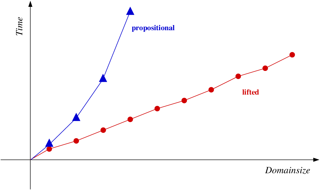
Van den Broeck 2011, therefore, has proposed a formal definition of domain lifted inference in terms of polynomial time complexity in the domainsize parameter. Experimental and theoretical analyses of existing lifted inference techniques then show that they provide domain lifted inference in some cases where basic propositional inference techniques would exhibit exponential complexity (as illustrated in Figure 1). However, until recently, these positive results were mostly limited to examples of individual models, and little was known about the feasibility of lifted inference for certain well-defined classes of models. First results that show the feasibility of lifted inference for whole classes of models are given by Van den Broeck 2011, and Domingos and Webb 2012.

On the other hand, Jaeger (2000) has shown that under certain assumptions on the expressivity of the modeling language, probabilistic inference is not polynomial in the domainsize, thereby demonstrating some inherent limitations in terms of worst-case complexity for the goals of lifted inference. However, the results of Jaeger (2000) are based on types of probabilistic logic models that are somewhat different from the models that presently receive the most attention: first, they essentially assume a directed modeling framework, in which the model represents a generative stochastic process for sampling relational structures. The model is defined by specifying marginal and conditional probability distributions for random variables corresponding to ground atoms. Ground instances of the model, then, can be represented by directed graphical models, i.e., Bayesian networks. While the majority of existing model classes fall into the category of directed models Breese (1992); Poole (1993); Sato (1995); Ngo et al. (1995); Jaeger (1997); Friedman et al. (1999); Kersting and Raedt (2001); Milch et al. (2005); Vennekens et al. (2006), there is currently a lot of interest in undirected models that are given by a set of soft constraints on relational structures, specified in the form of potential functions, and in the ground case giving rise to undirected graphical models, i.e., Markov networks. Secondly, the results of Jaeger (2000) require quite strong assumptions on the expressivity of the probabilistic-logic modeling language, which is required to allow that conditional distributions of atoms can be specified dependent on unrestricted first-order properties. Much current work, in contrast, is concerned with languages that only incorporate certain weak fragments of first-order logic.

In this paper the general approach of Jaeger (2000) is extended to obtain lower complexity bounds for inference in probabilistic-logic model classes that have emerged as the focus of interest for lifted inference techniques, i.e., undirected models based on quantifier- and function-free fragments of first-order logic.

In a sharp contrast with Jaeger (2000), where a “trivial” constant-time approximate inference method was described, we show that our lower complexity bounds also hold for approximate inference. Further sharpening earlier results, we finally establish that the lower complexity bounds also hold for models not using the equality predicate, which in Jaeger (2000) was conjectured to be the key source of inherent complexity.

A preliminary version of this paper has been published as Jaeger (2012). Its main results were also already included in the survey paper Jaeger and Van den Broeck (2012), which contains a systematic overview of known results and open problems related to the complexity of lifted inference.

In the following section we introduce a general framework in which classes of undirected probabilistic-logic models, and classes of associated inference problems can be defined. Section 3 reviews classic results relating first-order logic models to the complexity class NETIME. Section 4 contains our main results, and Section 5 discusses some notable differences that emerge between the results for directed and for undirected models.

Similarly as Richardson and Domingos (2006), Van den Broeck et al. (2011) and Gogate and Domingos (2011) we assume the following framework: a model, or knowledge base, is given by a set of weighted formulas:

where the $\phi_{i}$ are formulas in first-order predicate logic, $w_{i}\in\mathbb{R}$ are non-negative weights, and $\boldsymbol{v}_{i}=(v_{i,1},\ldots,v_{i,k_{i}})$ are the free variables of $\phi_{i}$. The case $k_{i}=0$, i.e., $\phi_{i}$ is a sentence without free variables, is also permitted. The $\phi_{i}$ use a given signature $S$ of relation-, function-, and constant symbols.

An interpretation (or possible world) $(D,I)$ for $S$ consists of a domain $D$, and an interpretation function $I$ that maps the symbols in $S$ to functions, relations and elements on $D$. For a tuple $\boldsymbol{d}\in D^{k_{i}}$ then the truth value of $\phi_{i}(\boldsymbol{v}_{i}/\boldsymbol{d})$ is defined, and we write $(D,I)\models\phi_{i}(\boldsymbol{d})$, or simpler $I\models\phi_{i}(\boldsymbol{d})$, if $\phi_{i}(/\ \boldsymbol{v}_{i}/\boldsymbol{d})$ is true in $(D,I)$. We use ${\cal I}(D,S)$ to denote the set of all interpretations for the signature $S$ over the domain $D$.

In this paper we are only concerned with finite domains, and assume without loss of generality that $D=D_{n}:=\{1,\ldots,n\}$ for some $n\in\mathbb{N}$.

For $I\in{\cal I}(D_{n},S)$ let $\#(i,I)$ denote the number of elements $\boldsymbol{d}$ in $D^{k_{i}}$ for which $I\models\phi_{i}(\boldsymbol{d})$. The weight of $I$ then is

where $0^{0}=1$. The probability of $I$ is

where $Z$ is the normalizing constant (partition function)

For a first-order sentence $\phi$ and $n\in\mathbb{N}$ then

is the probability of $\phi$ in ${\cal I}(D_{n},S)$.

We call a knowledge base (1) together with the semantics given by (2) and (4) a weighted feature model, since it associates weights $w_{i}$ with model features $\phi_{i}$. Weighted feature models in our sense can be seen as a slight generalization as weighted model counting (wmc) frameworks Fierens et al. (2011); Gogate and Domingos (2011) in which non-zero weights are only associated with literals. Knowledge bases of the form (1) can be translated into wmc frameworks via an introduction of new relation symbols $R_{1},\ldots,R_{n}$, hard constraints $\phi_{i}(\boldsymbol{v}_{i})\leftrightarrow R_{i}(\boldsymbol{v}_{i})$, and weighted formulas $R_{i}(\boldsymbol{v}_{i})\hskip 2.84526pt:\hskip 2.84526ptw_{i}$ Van den Broeck et al. (2011); Gogate and Domingos (2011). Up to an expansion of the signature, thus, weighted feature models and wmc are equally expressive. Markov Logic Networks Richardson and Domingos (2006) also are based on knowledge bases of the form (1) allowing arbitrary formulas $\phi_{i}$. However, the semantics of the model there depends on a transformation of the formulas into conjunctive normal form, and therefore does not exactly correspond to (2) and (4), unless the $\phi_{i}$ are clauses.

All types of models here discussed, thus, are very similar in nature, and only differ with respect to certain restrictions on what types of logically defined features can be associated with a weight. The general definition of weighted feature models gives us the flexibility of considering a variety of classes of such restrictions.

A probabilistic inference problem $\emph{PI}(\emph{KB},n,\chi,\eta)$ for a weighted feature model is given by a knowledge base KB, a domainsize $n\in\mathbb{N}$, and two first-order sentences $\chi,\eta$. The solution to the inference problem is the conditional probability $P_{\emph{KB},n}(\chi\mid\eta)$.

A class of inference problems is defined by allowing arguments $\emph{KB}$, $\chi$, and $\eta$ only from some restricted classes ${\cal KB}$, ${\cal Q}$ (the query class), and ${\cal E}$ (the evidence class), respectively. We use the notation

for classes of inference problems.

The results of this paper will be given for the case where ${\cal Q}$ consists of all ground atoms, denoted ${\cal AT}$, and ${\cal E}$ is empty. Thus, as far as ${\cal Q}$ and ${\cal E}$ are concerned, we are considering the most restrictive class of inference problems. Since we are deriving lower complexity bounds, this leads to the strongest possible results, which directly apply also to more general classes ${\cal Q}$ and ${\cal E}$.

Classes ${\cal KB}$ are defined by various syntactic restrictions on the formulas $\phi_{i}$ in the knowledge base. In this paper, we consider the following fragments of first-order logic (FOL): relational FOL (RFOL), i.e. FOL without function and constant symbols; 0-RFOL, which is the quantifier-free fragment of RFOL, and 0-RFOL^≠, which is 0-RFOL without the equality relation.

An algorithm solves a class $\emph{PI}({\cal KB},{\cal Q},{\cal E})$, if it solves all instances $\emph{PI}(\emph{KB},n,\chi,\eta)$ in the class. An algorithm $\epsilon$-approximately solves $\emph{PI}({\cal KB},{\cal Q},{\cal E})$, if for any $\emph{PI}(\emph{KB},n,\chi,\eta)$ in the class it returns a number $p\in[P_{\emph{KB},n}(\chi\mid\eta)-\epsilon,P_{\emph{KB},n}(\chi\mid\eta)+\epsilon]$. An algorithm that solves $\emph{PI}({\cal KB},{\cal Q},{\cal E})$ is polynomial in the domainsize, if for fixed $\emph{KB},\chi,\eta$ the computation of $\emph{PI}(\emph{KB},n,\chi,\eta)$ is polynomial in $n$.

The following definition introduces the central concept for our analysis.

The complexity class ETIME consists of problems solvable in time $O(2^{cn})$, for some constant $c$. The corresponding nondeterministic class is NETIME. Note that these classes are distinct from the more commonly studied classes (N)EXPTIME, which are characterized by complexity bounds $O(2^{n^{c}})$ Johnson (1990). For $n\in\mathbb{N}$ let $\emph{bin}(n)\in\{0,1\}^{*}$ denote the binary coding of $n$, and $\emph{un}(n)\in\{1\}^{*}$ the unary coding (i.e., $n$ is represented as a sequence of $n$ 1s). A set $S\subseteq\mathbb{N}$ is in (N)ETIME, iff $\{\emph{bin}(n)\mid n\in S\}$ is in (N)ETIME, which also is equivalent to $\{\emph{un}(n)\mid n\in S\}$ being in (N)PTIME.

Like Jaeger (2000), we use the following connection between spectra and NETIME as the key tool for our complexity analysis.

Thus, by reducing instances $n\in\emph{spec}(\phi)?$ of the spectrum recognition problem to probabilistic inference problems $\emph{PI}(\emph{KB},n,\chi,\eta)$, where $\emph{KB}\in{\cal KB},\chi\in{\cal Q},\eta\in{\cal E}$ are fixed for the given $\phi$, one establishes that the $\emph{PI}({\cal KB},{\cal Q},{\cal E})$ is not polynomial in the domainsize (under the assumption $\mbox{ETIME}\neq\mbox{NETIME}$).

This section contains our complexity results. We begin with a result for knowledge bases using full RFOL. This is rather straightforward, and (for exact inference) already implied by the results of  Jaeger (2000). We then proceed to extend this base result to 0-RFOL and 0-RFOL^≠.

There are some notable differences with respect to approximate inference between the results we here obtained for weighted model counting, and the results of Jaeger (2000). In Jaeger (2000) it was shown that due to convergence of query probabilities $P_{n}(a())$ as $n\rightarrow\infty$, in theory a trivial constant time approximation algorithm exists: perform exact inference for all input domains up to a size $n^{*}$, and output the limit probability for all domains of size $>n^{*}$. This “algorithm”, however, has no practical use, since for a desired accuracy value $\epsilon$ one first would have to determine a sufficiently high threshold value $n^{*}\in\mathbb{N}$ to make the output indeed be an $\epsilon$-approximation.

Nevertheless, the difference between the existence of an impractical approximation algorithm on the one hand, and the non-existence of any approximation algorithm on the other hand, is just one consequence of a more fundamental difference: while in the models considered in Jaeger (2000) query probabilities $P_{n}(a())$ converge to a limit, this is not necessarily the case for knowledge bases of weighted formulas – at least when full RFOL is allowed: in the proof of Theorem 4.1 we have constructed knowledge bases KB, such that $P_{\emph{KB},n}(a())$ oscillates between zero and values $>1/2$ as $n$ oscillates between $\emph{spec}(\phi)$ and its complement. The construction of knowledge bases with this behavior does not require formulas $\phi$ with a non-polynomial spectrum as in Corollary 3.4, and is not contingent on $\mbox{NETIME}\neq\mbox{ETIME}$. Already a knowledge base as constructed in the proof of Theorem 4.1 with $\phi$ replaced by $\psi$ of Example 3.2 will show this behavior.

The reason behind these different convergence properties lies in a somewhat different role that conditioning on evidence plays in directed and undirected models: in the former, a conditional probability $P_{M,n}(a()\mid b())$ defined by a model $M$ can, in general, not be defined as an unconditional probability $P_{M^{\prime},n}(a())$ in a modified model $M^{\prime}$. As a result, the convergence guarantees and – theoretical – approximability for certain classes of unconditional queries $P_{M,n}(a())$, do not carry over to conditional queries $P_{M,n}(a()\mid b())$.

For weighted feature knowledge bases $\emph{KB}$, on the other hand, there is no fundamental difference between unconditional and conditional queries $P_{\emph{KB}^{\prime},n}(a())$ and $P_{\emph{KB},n}(a()\mid b())$, respectively. To reduce the conditional to unconditional queries, one can just add to $\emph{KB}$ the hard constraint $\neg b()\hskip 2.84526pt:\hskip 2.84526pt0$ to obtain $\emph{KB}^{\prime}$ with $PP_{\emph{KB}^{\prime},n}=P_{\emph{KB},n}\mid b()$. This means that as long as ${\cal E}$ is not more expressive than ${\cal KB}$, the problem classes $\emph{PI}({\cal KB},{\cal Q},{\cal E})$ and $\emph{PI}({\cal KB},{\cal Q},\emptyset)$ have the same characteristics in terms of complexity as a function of the domainsize. Note, though, that this is only true when we consider complexity of $\emph{PI}(\emph{KB},n,\chi,\eta)$ strictly as a function of $n$ for fixed $\emph{KB},\chi,\eta$. If the evidence is allowed to change with the domainsize, i.e., $\eta=\eta(n)$, then even in cases where restrictions on ${\cal KB}$ make $\emph{PI}({\cal KB},{\cal Q},{\cal E})$ polynomial in $n$, one can define sequences of inference problems $\emph{PI}(\emph{KB},n,\chi,\eta(n))$ with $\emph{KB}\in{\cal KB}$, $\eta(n)\in{\cal E}$ that are no longer polynomial in $n$ Van den Broeck and Davis (2012).

We have shown that for currently quite popular probabilistic-logic models consisting of collections of weighted, quantifier- and function-free formulas there is likely to be no general polynomial lifted inference method (contingent on $\mbox{NETIME}\neq\mbox{ETIME}$). Somewhat surprisingly, this even holds for approximate inference. Between this negative result, and the positive result of Van den Broeck (2011), there still could be a lot of room for identifying tractable fragments by restricting 0-RFOL further via limits on the number of variables, or the richness of the signature $S$.

References

- Apsel and Brafman (2011) Apsel, U. and Brafman, R. I. 2011. Extended lifted inference with joint formulas. In Proceedings of the Twenty-Seventh Conference Annual Conference on Uncertainty in Artificial Intelligence (UAI-11). AUAI Press, 11–18.
- Breese (1992) Breese, J. S. 1992. Construction of belief and decision networks. Computational Intelligence 8, 4, 624–647.
- de Salvo Braz et al. (2005) de Salvo Braz, R., Amir, E., and Roth, D. 2005. Lifted first-order probabilistic inference. In Proceedings of the 19th International Joint Conference on Artificial Intelligence (IJCAI-05). 1319–1325.
- Domingos and Webb (2012) Domingos, P. and Webb, W. A. 2012. A tractable first-order probabilistic logic. In Proc. of AAAI-12. To appear.
- Fagin (1976) Fagin, R. 1976. Probabilities on finite models. Journal of Symbolic Logic 41, 1, 50–58.
- Fierens et al. (2011) Fierens, D., den Broeck, G. V., Thon, I., Gutmann, B., and Raedt, L. D. 2011. Inference in probabilistic logic programs using weighted cnf’s. In Proc. of UAI 2011.
- Friedman et al. (1999) Friedman, N., Getoor, L., Koller, D., and Pfeffer, A. 1999. Learning probabilistic relational models. In Proceedings of the 16th International Joint Conference on Artificial Intelligence (IJCAI-99).
- Gogate and Domingos (2011) Gogate, V. and Domingos, P. 2011. Probabilistic theorem proving. In Proceedings of the 27th Conference of Uncertainty in Artificial Intelligence (UAI-11).
- Jaeger (1997) Jaeger, M. 1997. Relational bayesian networks. In Proceedings of the 13th Conference of Uncertainty in Artificial Intelligence (UAI-13), D. Geiger and P. P. Shenoy, Eds. Morgan Kaufmann, Providence, USA, 266–273.
- Jaeger (2000) Jaeger, M. 2000. On the complexity of inference about probabilistic relational models. Artificial Intelligence 117, 297–308.
- Jaeger (2012) Jaeger, M. 2012. Lower complexity bounds for lifted inference. http://arxiv.org/abs/1204.3255.
- Jaeger and Van den Broeck (2012) Jaeger, M. and Van den Broeck, G. 2012. Liftability of probabilistic inference: Upper and lower bounds. In Proceedings of the 2nd International Workshop on Statistical Relational AI.
- Jha et al. (2010) Jha, A., Gogate, V., Meliou, A., and Suciu, D. 2010. Lifted inference seen from the other side: The tractable features. In Proc. of NIPS.
- Johnson (1990) Johnson, D. S. 1990. A catalog of complexity classes. In Handbook of Theoretical Computer Science, J. van Leeuwen, Ed. Vol. 1. Elsevier, Amsterdam, 67–161.
- Jones and Selman (1972) Jones, N. D. and Selman, A. L. 1972. Turing machines and the spectra of first-order formulas with equality. In Proceedings of the Fourth ACM Symposium on Theory of Computing. 157–167.
- Kersting and Raedt (2001) Kersting, K. and Raedt, L. D. 2001. Towards combining inductive logic programming with bayesian networks. In Proceedings of the 11th International Conference on Inductive Logic Programming (ILP-01). LNAI, vol. 2157. 118–131.
- Kisyński and Poole (2009) Kisyński, J. and Poole, D. 2009. Lifted aggregation in directed first-order probabilistic models. In Proc. of IJCAI 2009.
- Milch et al. (2005) Milch, B., Marthi, B., Russell, S., Sontag, D., Ong, D., and Kolobov, A. 2005. Blog: Probabilistic logic with unknown objects. In Proceedings of the 19th International Joint Conference on Artificial Intelligence (IJCAI-05). 1352–1359.
- Milch et al. (2008) Milch, B., Zettlemoyer, L. S., Kersting, K., Haimes, M., and Kaelbling, L. P. 2008. Lifted probabilistic inference with counting formulas. In Proceedings of the 23rd AAAI Conference on Artificial Intelligence (AAAI-08).
- Ngo et al. (1995) Ngo, L., Haddawy, P., and Helwig, J. 1995. A theoretical framework for context-sensitive temporal probability model construction with application to plan projection. In Proceedings of the Eleventh Conference on Uncertainty in Artificial Intelligence. 419–426.
- Poole (1993) Poole, D. 1993. Probabilistic horn abduction and Bayesian networks. Artificial Intelligence 64, 81–129.
- Poole (2003) Poole, D. 2003. First-order probabilistic inference. In Proceedings of the 18th International Joint Conference on Artificial Intelligence (IJCAI-03).
- Richardson and Domingos (2006) Richardson, M. and Domingos, P. 2006. Markov logic networks. Machine Learning 62, 1-2, 107 – 136.
- Sato (1995) Sato, T. 1995. A statistical learning method for logic programs with distribution semantics. In Proceedings of the 12th International Conference on Logic Programming (ICLP’95). 715–729.
- Singla et al. (2010) Singla, P., Nath, A., and Domingos, P. 2010. Approximate lifted belief propagation. In Proc. of AAAI-10 Workshop on Statistical Relational AI.
- Taskar et al. (2002) Taskar, B., Abbeel, P., and Koller, D. 2002. Discriminative probabilistic models for relational data. In Proc. of UAI 2002.
- Van den Broeck (2011) Van den Broeck, G. 2011. On the completeness of first-order knowledge compilation for lifted probabilistic inference. In Proc. of the 25th Annual Conf. on Neural Information Processing Systems (NIPS).
- Van den Broeck and Davis (2012) Van den Broeck, G. and Davis, J. 2012. Conditioning in first-order knowledge compilation and lifted probabilistic inference. In Proceedings of the Twenty-Sixth AAAI Conference on Articial Intelligence. 1961–1967.
- Van den Broeck et al. (2011) Van den Broeck, G., Taghipour, N., Meert, W., Davis, J., and Raedt, L. D. 2011. Lifted probabilistic inference by first-order knowledge compilation. In Proceedings of the 22nd International Joint Conference on Artificial Intelligence (IJCAI-11).
- Vennekens et al. (2006) Vennekens, J., Denecker, M., and Bruynooghe, M. 2006. Representing causal information about a probabilistic process. In Logics in Artificial Intelligence, 10th European Conference, JELIA 2006, Proceedings. Lecture Notes in Computer Science, vol. 4160. Springer, 452–464.