Casimir Energy For a Massive Dirac Field in One Spatial Dimension: A Direct Approach
Abstract
In this paper we calculate the Casimir energy for a massive fermionic field confined between two points in one spatial dimension, with the MIT Bag Model boundary condition. We compute the Casimir energy directly by summing over the allowed modes. The method that we use is based on the Boyer’s method, and there will be no need to resort to any analytic continuation techniques. We explicitly show the graph of the Casimir energy as a function of the distance between the points and the mass of the fermionic field. We also present a rigorous derivation of the MIT Bag Model boundary condition.
Keywords:
Casimir Energy; Fermion; MIT Bag ModelI Introduction
More than years have passed from the time when H. B. G. Casimir published his famous paper [1] on what has been called the Casimir effect ever since. It remained relatively unknown for over two decades, but from the early s this effect has attracted much attention. The Casimir energy is a pure quantum effect with macroscopic manifestations. Generally, the Casimir energy is defined as the difference between the vacuum energies in the presence and the absence of any external boundary conditions or background fields. Both of these energies are in general infinite. However the difference between the two has almost invariably been calculated to be finite. The Casimir effects have been calculated for a variety of fields, geometries, number of spatial dimensions, and boundary conditions (for a review see [2, 3, 4, 5]).
Recently the Casimir effect has been studied in connection with many physical phenomena. For example this effect has been studied in the context of the phenomenological chiral bag models of the nucleon [6, 7]. In such models the bag constant, , is an input parameter to the theory. As is well known, this constant is added to the Lagrangian density in order to balance the outward pressure of the quarks by the inward vacuum pressure on the surface of the bag [3]. This constant can be related to the Casimir energy [8]. The Casimir effect for the String and the Superstring leads to string theories having critical dimensions. The string is a finite two-dimensional system with an infinite phonon spectrum, the sum of the zero-point fluctuations of which leads to exactly the same calculation as in the original Casimir effect [9]. Moreover, the presence of the Casimir effects in many different phenomena in condensed matter and laser physics have been established both theoretically and experimentally [10, 11]. For example, the Casimir force is important in the development of microtechnologies that routinely allow control of separation between bodies smaller than [12, 13, 14]. An interesting application of the field theoretical models with compact dimensions recently appeared in nanophysics. The long-wavelength description of the electronic states in graphene can be formulated in terms of a Dirac-like theory in three dimensional space-time with the Fermi velocity playing the role of speed of light [15, 16, 17, 18, 19, 20]. Single-walled carbon nanotubes are generated by rolling up a graphene sheet to form a cylinder and the background space-time for the corresponding Dirac-like theory has topology [21].
In order to compute the Casimir energy, physically relevant boundary conditions must be imposed. For example the Casimir energy for an electromagnetic field is usually calculated with the boundary conditions appropriate for conducting boundaries as in [2, 3, 4, 5, 22, 23, 24, 25]. The Casimir energy for scalar fields has been investigated with the Dirichlet boundary condition [2, 3, 4, 5, 26, 27, 28, 29, 30], the Neumann boundary condition [3, 5], the mixed boundary condition [31], and the Robin boundary condition [32, 33, 34].
From this point on we concentrate on the Dirac field. Since the Dirac field obeys a first order differential equation of motion, it is impossible to use the aforementioned boundary conditions. Moreover, boundary conditions are in general more disruptive to Dirac fields than boson fields because the equations of motion are first order [35]. A proper boundary condition for the Dirac field is the MIT Bag Model boundary condition. It is usually said to imply that there is no flux of fermions through the boundary, i.e. if denotes the current of the Dirac field and is the normal unit vector to the boundary, then . However, it implies an even stronger condition which is the absolute confinement of the fermionic field. One could confine the fermionic wave function by an infinite scalar potential. This model was considered by Bogolioubov [36] and later developed as the MIT Bag Model by A. Chodos, et al [37, 38] for hadrons. It is important to mention that in general the computation of the Casimir energy for a massive Dirac field turns out to be much more difficult than the massless case. There has been relatively few studies for the Casimir energy inside closed surfaces, and we mentioned a few of them here. The Casimir energy has been calculated for a spherical geometry for a massive [39] and massless fermionic fields [3, 4, 40]. It has also been recently calculated for a massless fermionic field subject to the MIT Bag Model boundary condition confined inside a three dimensional rectangular geometry [41].
As usual there are many more studies on the two parallel plates geometry, and we shall concentrate on this problem from this point on. The first computation of the Casimir energy for the Dirac field was done by Johnson in [42]. He computed this energy per unit area for a massless fermionic field subject to the MIT Bag Model boundary condition between two parallel plates in three spatial dimensions. Afterwards, the Casimir energy has been calculated for massless fermions in one dimension [35], between two parallel plates using various methods in three-dimensional space [4, 3, 42, 43] and in dimensional space-time [44, 45, 46]. The first attempt to compute the Casimir energy for the massive case in three spatial dimensions was done by Mamayev and Trunov who managed to find an integral form for this quantity and explicitly computed its small and extremely large mass limits [47]. The first complete computation of the Casimir energy for the massive case in this geometry in and dimensions was done by C. D. Fosco and E. L. Losada in [48]. In their approach, a coupling of the bilinear form to a series of regularly spaced -function potentials with coupling constant is introduced, which implements imperfect bag-like boundary condition. This method can produce a fermionic propagator which satisfies the MIT Bag Model boundary condition when . However a direct calculation of the Casimir energy for this problem has not been presented so far, and this will be the subject of this paper.
In order to calculate the Casimir energy from first principles one must sum over the allowed modes. However, the vacuum energies in the presence and absence of disturbances obtained by these direct sums are infinite. Therefore one has to adopt regularization and analytic continuation prescriptions, in order to compute the difference between these two divergent quantities. When the allowed modes which appear in the summands are regular, the major approaches used are: the zeta function analytic continuation technique [4, 3, 34, 49], cut-off regularization [50, 51, 52, 53] and box subtraction scheme along with the Abel-Plana summation formula [27, 53]. On the other hand, when the allowed modes which appear in the summands are irregular, the major approaches used are: the contour integration method [54], the Green function formalism [55], the functional approach [48], and the Boyer method [56, 26]. Unfortunately, most of these techniques do not be lead to closed forms for the values of the Casimir energy and one has to employ various numerical methods to obtain a value for the Casimir energy.
In this paper we calculate the Casimir energy for a massive fermionic field in two dimensional space-time with the MIT Bag Model boundary condition, by directly summing over the modes. In this problem the fermionic modes are irregular and the divergences that appear are very severe. Upon using the contour integration method, one might encounter some ambiguities, mainly due to the severe nature of divergences inherent to this problem. Here we use a direct approach which does not resort to any analytic continuation techniques and is devoid of any ambiguities. Our method is based on the Boyer method, which we shall explain in detail [56]. Moreover, in this procedure one can associate a physical meaning to the Casimir energy: It is equal to the work done in forming the configuration under study from the free vacuum. In section II, we solve the Dirac equation in one spatial dimension using the MIT Bag Model boundary condition and we find a transcendental equation for the discrete spectrum. The allowed modes for the massive case obtained from this equation are not regular. In section III we compute the Casimir energy by performing a direct sum over all modes of the field. We finally plot the values obtained for the Casimir energy as a function of the distance between the points for various values of the mass. We show that the results for the small mass limit converges to the results for the massless case. The results obtained in this paper are consistent with those obtained in [48]. In Section IV we summarize our results. In the Appendix we present a rigorous derivation of the MIT Bag Model boundary condition for the most general case.
II The solution of Dirac Equation with the MIT Bag Model boundary condition
In this section we find the solutions to the Dirac equation with the MIT Bag boundary condition in one spatial dimension. We consider the case where the Dirac field is completely free inside the bag: . We can write the spinor as:
where denotes the energy eigenvalue of the time-independent solution. We choose the following representation for the -matrices: , , and . Then the Dirac equation leads to,
where .
The MIT Bag Model boundary condition has been derived in the Appendix A and we show that this boundary condition can completely confine the spinor fields between the boundaries. The MIT Bag Model boundary condition in two space-time dimension in our convention becomes,
| (8) |
Applying these conditions we obtain

Extracting from the condition and inserting it into , we obtain an expression which determines the quantized modes:
| (12) |
The above expression is identical to the result obtained by Mamayev and Trunov for the component of the momentum perpendicular to the plates for a massive Dirac field between two parallel plates in three spatial dimensions [47]. In Ref. [47] this condition has been obtained by using the MIT boundary condition and the property of the Dirac spinors that each component also satisfies the Klein-Gordon equation. However all of the allowed modes along with this equation for the two parallel plate geometry in 3+1 dimension can also be easily obtained directly, along the same lines as the derivation presented in this section. The solutions of the above transcendental equation (Eq. (12)), denoted by , are not regular for the massive Dirac fields. Only for the specific case of a massless Dirac field, the modes are regular (, ) [4, 3]. Since changing the sign of the root does not lead to a linearly independent solution, we consider only the positive roots.
As expected the MIT bag model boundary condition has transformed the spectrum of the free Dirac field, which consisted of two continua starting at , into two sets of discrete states with energies , where . This problem has parity symmetry and in this representation the parity operation is given by . The energy eigenstates automatically turn out to be parity eigenstates. The parities of the lowest lying states with energies are respectively, and the parities of the exited states alternate as the absolute value of the energy increases. The real and imaginary parts of the upper and lower components of the lowest two positive energy wavefunctions are plotted in Fig. (1). Note that the values of the wavefunctions on the boundaries are non-zero and just outside the boundaries are exactly zero. This is another manifestation of the imposition of the MIT bag model boundary condition, as explained fully in the Appendix A.
In order to calculate the Casimir energy for the massive case we need to find a relationship between the root number and the wave number . For this purpose, Eq. (12) can be written as:
| (13) |
where is the root number, and . Note that the values of the root indices and the corresponding wave-numbers can be analytically continued to any real value.
III The Casimir Energy
In this section we calculate the Casimir energy for a massive Dirac field between two parallel plates (two points) in 1+1 space-time dimensions. In order to obtain the Casimir energy, we should subtract the zero point energy in the absence from the presence of the boundary conditions. Therefore, the vacuum energies for both cases should be calculated. Since the solutions of the Hamiltonian in the absence and presence of the boundaries are complete [58, 59], the Fermi field operator can be expanded in terms of either of these modes, as follows
| (14) | |||||
where we have denoted the positive-energy and negative-energy modes in the free case by and , and in the case with the boundary condition by and , respectively. By substituting the expressions for the field operator given in Eq. (14) into the general definition of the Hamiltonian operator and using the usual anticommutation relations, and evaluating the two zero point energies, we obtain the following expression for the Casimir energy,
| (15) | |||||
where and denote the vacuum states in the absence and the presence of the boundary condition, respectively. We have just shown that we can obtain the vacuum energy, and therefore the Casimir energy, by simply summing over the negative energy modes without the factor of . This is equivalent to the usual definition where one sums over both positive and negative energy modes, since our problem possesses particle conjugation symmetry along with C, P and T symmetries, separately. Integrating over the Casimir energy becomes,
| (16) |
As mentioned earlier both of these vacuum energies are infinite. However the difference, which is the Casimir energy, is expected to be finite. In many of the techniques for calculating the Casimir energy one starts with only the expression for the vacuum energy for the problem at hand (the first expression in Eq. (16) in our case) and removes the infinities that appear during the calculation by using various methods such as analytic continuation or simply by hand. this should precisely amount to subtracting the free vacuum energy which was left out from the beginning (the second expression in Eq. (16) in our case).
The dependence of the fermionic quantized momenta on the mass of the field is one of the distinguishing features of the Fermi field as compared to the bosonic case. In Fig. (2) we show the wave vectors for two massive and a massless fermionic field.
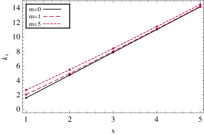
However as mentioned earlier, for the wave vectors are evenly spaced and are given by . Therefore the Casimir energy for a massless fermionic field can be easily obtained from the first term in Eq. (16) using the zeta function and its analytic continuation as follows [3, 35],
| (17) | |||||
As shown in Fig. (2) the wave numbers obtained from Eq. (12) for a massive Dirac field are irregular. In order to calculate the Casimir energy we use the Boyer method [56], instead of using Eq. (16) directly, since the latter is more prone to ambiguities. These two methods for calculating of the Casimir energy are equivalent. Now we discuss the Boyer method in detail. In this method we consider two similar configurations: two points with distance and two points with distance . Then we place each of these systems in a box with size as Fig. (3). Finally we define the Casimir energy as the difference between the vacuum energies of these two similar configurations as follows,
| (18) |

where and are the vacuum energies of configurations ‘A’ and ‘B’ as shown in Fig. (3). Note that upon taking the limits indicated in Eq. (18), one recovers the original definition of the Casimir energy given in Eq. (16). From this definition one can easily conclude that the Casimir energy is equal to the work done on the configuration ‘B’ to deform it to configuration ‘A’. For each of the six regions shown in the Fig. (3), for example the region , we calculate the vacuum energy as follows,
| (19) |
where we have introduced a convergence factor with . Now we start the calculation for the region , and the calculations for the other regions can be done analogously. Since the wave-vectors are not regular with respect to the root indices , in order to find an analytical form for the divergence in Eq. (19), we employ the simplest form of the Euler-Maclaurin Summation Formula (EMSF) to obtain
| (20) | |||||
where is the Floor function. There is a one-to-one correspondence between the wave vector and the root number , as is manifest in Eq. (13). Therefore we can change the variable of integration from to . Then we obtain,
| (21) | |||||
Now, by adding and subtracting appropriate terms, we can extend the lower limits of all integrals in Eq. (21) to zero. We thus have
| (22) | |||||
The last term in Eq. (22) can be simplified by noting that the Floor function in the indicated domain, and integration by parts yields,
| (24) | |||||
Note that only the first term on the right hand side of Eq. (24) is divergent. Upon substituting the expression displayed in Eq. (24) into the definition of the Casimir energy given in Eq. (18), the constant terms automatically cancel each other in the limit and by choosing appropriate cutoffs on the upper limits of the integrals for each region, the divergent integrals cancel each other, all due to the box subtraction scheme. Therefore only the convergent integral terms remain. The contributions of integrals in regions , and go to the zero as and . Therefore our final expression for the Casimir energy is,
| (25) |
where is obtained from Eq. (13). It seems that this expression does not have a closed form solution and it should be solved numerically. As is apparent from Eq. (25), the integrand has an infinite number of discontinuities due to the presence of the Floor function. First the precise positions of the jumps in the integrand have to be determined. These jumps precisely correspond to the roots of Eq. (12), giving the values of the wave-numbers. The integrations are done separately for all parts and then all of the results are summed. The integration is over the continuous version of the wave number, which extends to infinity. In order to accomplish this numerically, we compute this integral up to a cutoff which should eventually go to infinity. Meanwhile, we also have to take the limit as indicated in Eq. (25). We have determined that an optimization occurs precisely when . In Fig. (4) the values of the Casimir energy have been plotted as a function of the distance for various values of . This plot shows that there is a good consistency between the results of the massless case and massive ones when . This figure also shows the rapid decrease in the value of the Casimir energy as a function of . We should mention that our results are in an excellent agreement with the previously reported result which was obtained indirectly through the analysis of the bilinear forms [48].

IV Conclusion
In this paper we have computed the Casimir energy for a massive Dirac field with the MIT Bag Model boundary condition in one spatial dimension. We have used the direct mode summation method in order to compute the Casimir energy for this field. For the massless case the modes are regular and we use the zeta function analytic continuation technique. However, for the massive case the modes are irregular and we use the Boyer’s subtraction scheme. Its worth mentioning that in this technique all of the infinities are canceled automatically and there is no need to use any analytic continuation. We have shown that the massless limit of the massive case precisely corresponds to the massless case. Our result for the values of the Casimir energy has been obtained numerically, similar to the previously reported results [48].
Acknowledgement
We would like to thank the Research Office of the Shahid Beheshti University for financial support.
Appendix A A Derivation for the MIT Bag Model Boundary condition
In this appendix we present a rigorous derivation of the MIT Bag Model boundary condition for the Dirac field inside an arbitrary closed surface . This boundary condition ensures the complete confinement of the eigenstates of the Dirac Hamiltonian inside an enclosed area. We show that this boundary condition can be obtained by coupling the Dirac field to a scalar potential and taking the limit as . However we first present the reasons why we cannot confine fermions inside an enclosed area by the time component of a four-vector potential .
Solving the Dirac equation we obtain which is positive for . Therefore we have oscillatory solutions out of the barrier, i.e. we have currents of particles and antiparticles. This contradicts the assumption of complete confinement of the fermionic field. This is the well-known Klein’s paradox [57]. Next we use the scalar potential which, as we shall see, does not have this problem. The Dirac equation with the scalar potential is:
| (26) |
Decomposing the spatial components of at the surface into tangential and normal parts, we have:
| (27) |
We choose the potential to be infinite outside of the enclosed area and to vanishes inside. First we take the integral of the Dirac equation with the scalar potential (Eq. (26)) from to (a small interval inside the barrier) where specifies a random point on the surface and is the normal unit vector to the surface at point
| (28) |
When , all of the terms vanish except the one containing the term . Then:
| (29) |
Second, we change the integration domain. This time we integrate from a point just inside the volume () to a point outside of the volume ().
| (30) |
This time we have to deal with the infinite potential outside the bag and therefore we cannot neglect the term . Now using the fact that the Dirac equation demands and Eq. (29) one obtains:
| (31) |
Multiplying Eq. (31) from left by yields . Since and we conclude .
It is interesting to note that using the time component of a four-vector potential for the confinement purpose we obtain an inconsistent result: .
Inserting in Eq. (31) we obtain the MIT Bag Model boundary condition:
| (32) |
References
- [1] H. B. G. Casimir, Proc. Kon. Nederl. Akad. Wet. 51 (1948) 793.
- [2] M. Bordag, G.L. Klimchitskaya, U. Mohideen, and V.M. Mostepanenko, Advances in the Casimir Effect, Oxford University Press Inc. New York (2009).
- [3] K. A. Milton, The Casimir Effect: Physical Manifestations of Zero-Point Energy, (World Scientific Publishing Co. Pte. Ltd. 2001).
- [4] K. A. Milton, The Casimir Effect: Physical Manifestations of Zero Point Energy, Invited Lectures at 17th Symposium on Theoretical Physics, Seoul National University, Korea, June 29-July 1, (1998); [arXiv:hep-th/9901011v1].
- [5] M. Bordag, U. Mohideen, V.M. Mostepanenko, Phys. Rep. 353 (2001) 1; [arXiv:quant-ph/0106045v1].
- [6] Hee-Jung Lee, Dong-Pil Min, Byung-Yoon Park, Mannque Rho and Vicente Vento, Nucl. Phys. A 657 (1999) 75.
- [7] Linas Vepstas, A. D. Jackson and A. S. Goldhaber, Nucl. Phys. B 140 (1984) 280.
- [8] I. O. Cherednikov, Int. J. Mod. Phys. A 17, 874 (2002).
- [9] L. Brink and H. B. Nielsen, Phys. Lett. B 45, 332 (1973).
- [10] F. De Martini, M. Marrocco and P. Mataloni, Phys. Rev. A 43, 2480 (1991).
- [11] M. Krech and S. Dietrich, Phys. Rev. Lett. 66, 345 (1991).
- [12] F. Chen, U. Mohideen, G. Klimchitskaya and V. Mostepanenko, Phys. Rev. Lett. 88 (2002) 101801.
- [13] R. Rodrigues, P. Maia Neto, A. Lambrecht and S. Reynaud, EPL 76, 822 (2006).
- [14] A. Lambrecht, I. Pirozhenko, L. Duraffourg and Ph. Andreucci, EPL 77, 44006 (2007).
- [15] G.W. Semenoff, Phys. Rev. Lett. 53, (1984) 2449.
- [16] D.P. Di Vincenzo and E.J. Mele, Phys. Rev. B 29 (1984) 1685.
- [17] J. González, F. Guinea, and M. A. H. Vozmediano, Phys. Rev. B 63 (2001) 134421.
- [18] H.-W. Lee and D.S. Novikov, Phys. Rev. B 68 (2003) 155402.
- [19] S.G. Sharapov, V.P. Gusynin, and H. Beck, Phys. Rev. B 69 (2004) 075104.
- [20] A.H. Castro Neto, F. Guinea, N.M.R. Peres, K.S. Novoselov, and A.K. Geim, Rev. Mod. Phys. 81 (2009) 109.
- [21] S. Bellucci and A. A. Saharian, Phys. Rev. D80 (2009) 105003; [arXiv:hep-th/0907.4942v1]
- [22] J. Ambjørn, and S. Wolfram, Ann. Phys. (N. Y.) 147 (1983) 1.
- [23] M. A. Valuyan, R. Moazzemi, and S. S. Gousheh, J. Phys. B: At. Mol. Opt. Phys. 41 (2008) 145502; [arXiv:hep-th/0806.1628].
- [24] S. Hacgan, R. Jáuregui, and C. Villarreal, Phys. Rev. A 47 (1993) 4204.
- [25] G. Jordan Maclay, Phys. Rev. A 61 (2000) 052110-1.
- [26] M. A. Valuyan, and S. S. Gousheh, Int. J. Mod. Phys. A 25 (2010) 1165.
- [27] R. Moazzemi, M. Namdar, and S.S. Gousheh, JHEP 09 (2007) 029; [arXiv:hep-th/0708.4127v1].
- [28] R. Moazzemi, and S. S. Gousheh, Phys. lett. B 658 (2008) 255; [arXiv:hep-th/0708.3428v2].
- [29] S. S. Gousheh, R. Moazzemi, and M. A. Valuyan, Phys. Lett. B 681 (2009) 477; [arXiv:hep-th/0911.3707].
- [30] R. Moazzemi, Abdollah Mohammadi, and S.S. Gousheh, Eur. Phys. J. C 56 (2008) 585; [arXiv:hep-th/0806.4862].
- [31] A. C. Aguiar Pinto, T. M. Britto, R. Bunchaft, F. Pascoal, and F.S.S. da Rosa, Brazilian Journal of Physics 33 (2003) 60.
- [32] A. Romeo, and A. A. Saharian, J. Phys. A: Math. Gen. 35 (2002) 1297; [arXiv:hep-th/0007242v2].
- [33] L.C. de Albuquerque, and R. M. Cavalcanti, J. Phys. A: Math. Gen. 37 (2004) 7039; [arXiv:hep-th/0311052v2].
- [34] C. Farina, Brazilian Journal of Physics 36 (2006) 1137.
- [35] P. Sundberg, and R. L. Jaffe, Ann. Phys. 309 (2004) 449; [arXiv:hep-th/0308010v1].
- [36] P. N. Bogolioubov, Ann. Inst. Henri Poincare 8 (1967) 163.
- [37] A. Chodos, R. L. Jaffe, K. Johnson, C. B. Thorn, and V. F. Weisskopf, Phys. Rev. D 9 (1974) 3471.
- [38] A. Chodos, R. L. Jaffe, K. Johnson, and C. B. Thorn, Phys. Rev. D 10 (1974) 2599.
- [39] E. Elizalde, M. Bordag, and K. Kirsten, J. Phys. A: Math. Gen. 31 (1998) 1743; [arXiv:hep-th/9707083v1].
- [40] R. Hofmann, M. Schumann and R.D. Viollier, Eur. Phys. J. C 11 (1999) 153.
- [41] A. Seyedzahedi, R. Saghian, and S. S. Gousheh, Phys. Rev. A.82 (2010) 032517.
- [42] K. Johnson, Acta. Pol. B 6 (1975) 865.
- [43] H. Queiroc, J. C. da Silva, and F. C. Khanna, J.M.C. Malbouisson, M. Revzen and A. E. Santana, Ann. Phys. 317 (2005) 220.
- [44] E. Elizalde, F. C. Santos, and A. C. Tort, Int. J. Mod. Phys. A 18 (2003) 1761; [arXiv:hep-th/0206114v1].
- [45] A. A. Saharian and M. R. Setare, Int. J. Mod. Phys. A 19 (2004) 4301.
- [46] A. A. Saharian and E. R. Bezerra de Mello, Int. J. Mod. Phys. A 20 (2005) 2380.
- [47] S. G. Mamayev and N. N. Trunov, Sov. Phys. J 23 (1980) 551.
- [48] C. D. Fosco, and E. L. Losada, Phys. Rev. D 78 (2008) 025017; [arXiv:hep-th/0805.2922v1].
- [49] E. Elizalde, S. D. Odindsov, A. Romeo, A. A. Bitsenko and S. Zerbini, Zeta Regularization Techniques with Appliccations, (World Scientific, Singapore, 1994).
- [50] N. F. Svaiter, and B. F. Svaiter, J. Phys. A: Math. Gen. 25 (1992) 979.
- [51] M. S. R. Milto, Phys. Rev. D 78 (2008) 065023.
- [52] C.R. Hagen, Eur. Phys. J. C 19 (2001) 677.
- [53] A. A. Saharian, The generalized Abel-Plana formula: applications to Bessel functions and casimir effect, [arXiv:hep-th/0002239v1].
- [54] V. V. Nesterenko and I. G. Pirozhenko, Phys. Rev. D 57 (1998) 2.
- [55] K. A. Milton, L. L. Deraad, and J. Schwinger, Ann. Phys. (N.Y.) 115, 388 (1978).
- [56] T. H. Boyer, Phys. Rev.174 (1968) 1764.
- [57] J. J. Sakurai, Advanced Quantum Mechanics, Addison Wesley; Rev sub edition (1993).
- [58] R. MacKenzie and F. Wilczek, Phys. Rev. D 30, 2194 (1984).
- [59] S. S. Gousheh and R. López-Mobilia, Nucl. Phys. B 428, 189 (1994).