Quantum Decoherence of the Central Spin in a Sparse System of Dipolar Coupled Spins
Abstract
The central spin decoherence problem has been researched for over 50 years in the context of both nuclear magnetic resonance and electron spin resonance. Until recently, theoretical models have employed phenomenological stochastic descriptions of the bath-induced noise. During the last few years, cluster expansion methods have provided a microscopic, quantum theory to study the spectral diffusion of a central spin. These methods have proven to be very accurate and efficient for problems of nuclear-induced electron spin decoherence in which hyperfine interactions with the central electron spin are much stronger than dipolar interactions among the nuclei. We provide an in-depth study of central spin decoherence for a canonical scale-invariant all-dipolar spin system. We show how cluster methods may be adapted to treat this problem in which central and bath spin interactions are of comparable strength. Our extensive numerical work shows that a properly modified cluster theory is convergent for this problem even as simple perturbative arguments begin to break down. By treating clusters in the presence of energy detunings due to the long-range (diagonal) dipolar interactions of the surrounding environment and carefully averaging the effects over different spin states, we find that the nontrivial flip-flop dynamics among the spins becomes effectively localized by disorder in the energy splittings of the spins. This localization effect allows for a robust calculation of the spin echo signal in a dipolarly coupled bath of spins of the same kind, while considering clusters of no more than six spins. We connect these microscopic calculation results to the existing stochastic models. We, furthermore, present calculations for a series of related problems of interest for candidate solid state quantum bits including donors and quantum dots in silicon as well as nitrogen-vacancy centers in diamond.
pacs
03.65.Yz; 76.30.-v; 76.60.Lz; 03.67.LxI Introduction
The problem of decoherence of a spin interacting with a bath of spins (the “central spin problem”) has its roots in classic works on electron and nuclear magnetic Resonance (see Ref. 1 and references cited therein). In these early works, the dynamics of an ensemble of spins being resonant with external control field (spin species A), and interacting with a larger ensemble of off-resonant spins (species B), was considered. The fluctuations of the B spins (due to their mutual spin-spin interactions and due to spin-lattice relaxation) leads to precession frequency fluctuations of the A spins (the spectral diffusion), which were then modeled as a classical stochastic process. Spin echo (SE) signals of A spins were calculated using different assumptions about the statistical properties of this process.[2, 3, 4]
The central spin decoherence problem has received renewed attention due to emergence of ideas for using localized spins in solid state systems as qubits in a quantum computer. The currently studied systems include gate-defined quantum dots,[5] self-assembled quantum dots,[6, 7] phosphorous donors in silicon,[7] and nitrogen-vacancy (NV) centers in diamond.[8] In all of these systems, the coupling of the central (qubit) spin to a bath of other spins is the dominant process of the loss of coherence in a superposition of spin up and down states (i.e., dephasing).
A lot of attention has been recently devoted to the problem in which the electron spin is coupled by a contact hyperfine (hf) interaction to a bath of nuclear spins. For large magnetic fields only the longitudinal part of this interaction should be relevant (due to a large Zeeman splitting mismatch between the electron and nuclear spins suppressing their mutual flip-flops), and the decoherence of the qubit should occur due to intrinsic fluctuations of the nuclear spins caused by their mutual dipolar coupling. Quantitative comparison between theory[1, 9, 10, 11] and experiments for spin echo in Si:P (see Refs. 12, 13, 14, 15) and Si:Bi (see Ref. 16) systems has shown that for natural concentration of spinful isotope of 29Si this is indeed the case. The same origin of spin echo decay was predicted for electron spins in III-V compound based quantum dots in the regime of large magnetic fields.[10, 17, 18] Recent experiments[19] in GaAs singlet-triplet qubit agree with these calculations for magnetic fields higher than T. At lower fields, the electron-nuclear spin flip-flops cannot be completely ignored, and the SE decay is dominated by the contact hf interaction,[20, 21, 22] with dipolar dynamics being only a correction.
The case of a purely dipolarly coupled system, more closely analogous to the original spectral diffusion problem, was also recently brought back into focus by developments in spin qubit physics. One motivation is the fact that silicon can be isotopically enriched to reduce the concentration of spinful 29Si. Below a certain concentration threshold, one can expect that the dipolar interactions between the electron spins themselves will limit the coherence time. In fact it was pointed out years ago that at large P concentrations the decay of the observed SE signal of the donor-bound electrons might decay due to dipolar interactions between these electron spins.[3] A theory addressing the range of currently studied small concentrations of both P donors and the 29Si nuclei was proposed recently.[23] In that work, it was shown that (1) the SE decay time in Si:P is bounded by a few seconds due to long-range dipolar interactions between electron spins for realistically small donor concentrations (about cm-3) and (2) the presence of some 29Si can actually increase the time considerably by suppressing donor-induced decoherence. The latter effect is due to the nuclei providing quasi-static Overhauser shifts of electron spin splittings, which increase the detunings between the electron spins, and suppress the dipolar flip-flop dynamics in the bath.[24] The predictions of Ref. 23 for SE decay times have been recently confirmed experimentally.[25]
Another system for which both the qubit-bath and the intrabath couplings are of the dipolar origin is the nitrogen-vacancy (NV) center in diamond.[8, 26, 27, 28, 29, 30, 31] In this case, decoherence of the qubit (which is made out of two levels of an electronic spin triplet) is dominated either by interaction with a bath of electron spins of nitrogen atoms (so-called P1 centers), as in Refs. 27 and 29, or, in the case of purer samples, by interaction with a bath of nuclear spins of 13C atoms, as in Refs. 26, 28, and 31.
In this paper we present a detailed description of a cluster-based theory applicable to a sparse dipolarly coupled system,[23] and we give multiple examples of applications of the theory. In order to put this work into context, let us briefly review the modern microscopic approaches to spectral diffusion (for an attempt at pedagogical introduction to these theories see Ref. 32). A method using a cluster expansion of bath dynamics was developed in Refs. 9 and 10 and applied in the context of spin qubit decoherence in semiconductors. This theory produced results in remarkable agreement with experimental spin echo decay measurements using only well-known microscopic (no fitting) parameters. [33] Various theories of this type have been applied to problems in which an electron spin decoheres due to contact hf interactions with a dynamical nuclear spin bath.[9, 10, 17, 34, 35, 33, 36] In all of these works based upon cluster expansions of some form, the contributions of the bath dynamics to central spin decoherence were grouped according to the number of bath spins participating in a nontrivial way (e.g., undergoing flip-flop processes). In all of these nuclear-induced spectral diffusion problems, the coupling of the central electron spin to nuclear spins is typically much larger than dipolar interactions that couple the nuclear spins to each other. The cluster expansions are essentially perturbative expansions in the intra-bath coupling, (related to a diagrammatic linked cluster expansion[11] but less cumbersome to compute numerically) and are therefore well suited to problems in which these interactions are relatively weak. Problems in which the interactions among bath spins are comparable to their interactions with the central spin (e.g., sparse, dipolar coupled electron spins) present a challenge for these cluster methods. In this article, we show that we can adapt the cluster correlation expansion (CCE) of Refs. 37 and 38 to treat these problems successfully. The CCE of Refs. 37 and 38 is essentially equivalent to the original cluster expansion [9, 10] but greatly simplified and more convenient for considering large cluster corrections. This method was recently applied to the NV center coupled to the nuclear spin bath where it was used to predict interesting effects related to the qubit back-action on the bath dynamics.[39, 40, 31] Without relying upon the large-bath approximations or cumbersome corrections of the earlier cluster expansion theory,[10] or relying upon the clustered grouping approximation of the disjoint cluster approach,[36] the CCE is well suited for including larger spin clusters. These larger clusters need to be calculated when considering dynamical decoupling of the central spin[41, 42], or when the bath is sparse and multi-spin correlations build within it on the timescale of the central spin decoherence. The latter case applies to the problem that is the focus of this article.
It may appear at first that the cluster expansion, which depends critically on the higher order clusters making systematically weaker contributions to decoherence in a parametrically well-behaved manner, would be completely impractical for problems involving a sparse bath of environmental spins and/or a bath environment containing similar spins to the central spin. One may wonder that in either case (i.e., sparse bath or qubit-bath interaction being the same as the intra-bath interaction), it may simply be impossible to define “clusters” in any meaningful manner for a reasonable cluster expansion technique to work. In fact, this has inhibited the application of the cluster expansion technique, in spite of its great success in the standard spectral diffusion problem of spin decoherence in Si and GaAs, to a number of important problems of increasing experimental importance. In the current work, we establish the applicability of a cluster expansion technique for the central spin decoherence problem for a sparse bath with strong intra-bath couplings (comparable to bath-qubit couplings). Once such a theoretical technique is established, we can then solve a number of central spin quantum decoherence problems of current experimental relevance using it, and we apply the technique to solve several problems of interest in Si and diamond quantum computing architectures.
The key insight, which follows from a careful implementation of the CCE to the sparse dipolar bath and from extensive numerical calculations involving increasing cluster sizes, is our finding of an effect of localization of flip-flop dynamics of bath spins that is not obvious a priori. For any given group (cluster) of spins, their mutual energy detunings are affected by the state of all the other spins, outside of the cluster. This is due to the diagonal () part of the dipolar interaction. Our calculations show that in a sparse dipolarly coupled bath these interactions are introducing strong disorder in the energy splittings of bath spins. This disorder suppresses the contribution from larger cluster sizes in an appropriately modified CCE. We find that the CCE can be adapted to converge well for a sparse dipolar bath by defining cluster contributions to include these externally-induced energy splittings and to be effectively, but efficiently, averaged over internal and external spin states. (We note that Ref. 17 had previously included effects of externally-induced energy splittings in its pair approximation). The results and the convergence can be strongly dependent upon the arrangement of bath spins, but the convergence of results that are averaged over different spatial realizations of the bath is well controlled. In our modified formulation of the CCE, we can obtain convergent results for SE decay up to times at which the coherence had decayed by an order of magnitude while calculating clusters of at most four spins (with six spins clusters being shown to contribute a negligible correction at this timescale).
Our main focus is thus the case of a central spin coupled to the bath spins of the same kind by dipolar interaction, e.g. an electron spin coupled to other electron spins. Such a situation has been extensively studied theoretically by Dobrovitski et al. in Refs. 43, 44, 27 and 29. The most important conclusion of these papers, based on extensive comparison between exact numerical calculations, stochastic model, and diverse experiments for NV center coupled to electron spins, is that the decoherence of a single NV center (coupled to an electron spin bath) can be modeled very well by replacing the bath by a source of classical Ornstein-Uhlenbeck noise.[27, 44, 29] For spin echo this means decay of the form crossing over at long times to . An important distinction[43] was also made between the results of experiments on an ensemble of qubits, and results obtained by repeated measurement of the same qubit (as it is done in experiments on a single NV center). This distinction is very important for our work here: we consider both cases (the ensemble of qubits, and a single qubit), since the first of them is important for current experiments on Si:P, while the second is relevant for current NV center experiments as well as considerations for addressable quantum bits. It is important to note that these studies using exact numerics are limited to very small bath sizes (tens of spins with current computing technology) and that cluster expansions do not have that limitation.
The paper is organized in the following way. In Sec. II, we describe the Hamiltonian of the system of interest, a central spin dipolarly coupled to an ensemble of randomly positioned spins, all of them also coupled by dipolar interactions, and define the coherence measurement procedure (the spin echo) which our theory addresses. In Sec. III, we provide a detailed description of a variant of cluster expansion theory applicable to such a problem. There we give all the details of the theory used in Ref. 23 to predict the 29Si and P concentration dependence of the electron spin coherence time is Si:P system. In Sec. IV, we describe many interesting and experimentally relevant variations of the “canonical” problem defined in Sec. II. There we discuss the role of the intra-bath coupling strength relative to their interactions with the central spin, the possible geometrical variants of the problem (i.e., the case of the bath spins being localized in a plane some distance from the central spin), and generalizations of spin echo experiment to sequences of multiple pulses (dynamical decoupling). Finally, in Sec. V, we present theoretical results for many example systems: donor-bound electrons in bulk silicon or near an interface, Si-based quantum dots, and NV centers in diamond.
II Canonical Problem: Decoherence in a Sparse All-Dipolar Spin System
In this section, we describe our canonical problem of interest, the spin echo decoherence of a central spin in a sparse all-dipolar spin-1/2 system in a strong, homogeneous magnetic field environment. In this canonical problem, we assume that the central spin is shifted off of resonance from the spins of the bath, but relax this assumption for one of the variants in Sec. IV. Using spin-1/2 particles is relevant for applications to electron spin systems; however, our methods equally capable of treating spins of larger magnitude.
II.1 System of spins
For our canonical problem, we consider a sparse system of electron spins uniformly distributed at random in a three-dimensional continuum (or on a lattice in which the diluteness of the spins makes the lattice structure irrelevant). The electrons are localized (bound to donors, for example) and dilute to the extent that they may be treated as point dipoles. In fact, it is not essential that they be electrons, but we employ conventions of notation (such as -factor) that are consistent with electron particles. We also assume the existence of a uniform magnetic field that we choose, for convention, to lie along the “z” direction. Our Hamiltonian, written in atomic units ( and ), is thus
| (1) |
where are spin operators for the spin-1/2 particles, is the Bohr magneton, is the g-factor of the th electron (typically, ), is the externally applied magnetic field at each electron site, and is a tensor to characterize dipolar interactions and is defined by
| (2) |
with . is the Kronecker delta and is the vector component of . Our convention is to index the central spin as .
For our canonical problem, we set and take the limit of a large applied magnetic field that is equal among all bath spins but different for the central spin. That is, all except the central spin are on resonance with each other (neglecting at this point the energy offsets due to dipolar interactions). If our central spin represents a quantum bit, it makes sense that we would be able to address it individually and shift its Zeeman energy to be off resonant from the bath spins. In taking this limit of a large applied magnetic field, we should disregard interactions which do not preserve the net Zeeman energy (the secular approximation). Thus, our effective Hamiltonian for our canonical problem becomes
| (3) |
with
| (4) |
where is the angle that the vector from spin to spin makes with the “z” unit vector (the direction of applied magnetic field) and is the length of this vector. By forcing the magnetic field of the central spin to be different from the rest and taking the large field limit, we suppress any flip-flopping between the central spin (with index zero by our convention) and bath spins. This is, then, a standard spectral diffusion problem in which the polarization of the central spin is preserved but the qubit will dephase due to bath-induced variations of its precessional frequency (i.e., its spectral line “diffuses”). We later treat the case in which the central spin is resonant with the bath spins in Sec. IV.1.
Note that the effective Hamiltonian of Eq. (3) has a 1/ dependence entirely. The entire Hamiltonian, therefore, scales with the concentration of the spins (). The dynamics is therefore scale invariant, with time that scales inversely with the . Likewise, time scales inversely with the square of the g-factors. Our results, unless otherwise specified, apply to a bath of and . However, adjusting these parameters only serves to rescale the time axis.
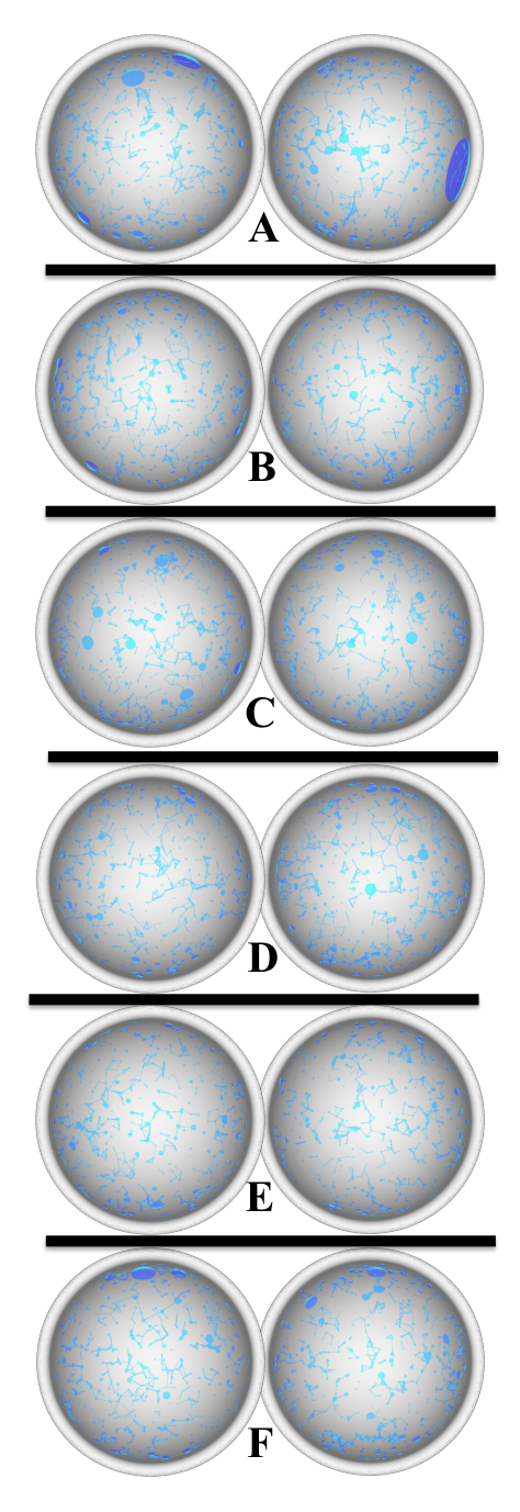
Since we are specifying that the spins are at random positions in space, there are many spatial realizations of this problem. As a way to visualize a particular instance of a spatial realization of the problem, we use “celestial map” diagrams as shown in Fig. 1. These diagrams represent each particular “universe” from the perspective of a central spin. Positions of the bath spins are projected onto a sphere (centered at the central spin) as cylinders whose size is proportional to the strength of the interaction with the central spin. The left and right hemispheres are split apart so we can look out in any direction from the central spin. We connect the representatives of the bath spins with rods in proportion to the strength of their mutual interaction as well as their interactions to the central spin (where these interactions are beyond some criteria in strength). In these way, we get effective “constellations” of bath spins. We chose six random instances labeled A through F depicted in Fig. 1, and will refer to these by letter throughout the text.
We consider the limit of an infinite bath temperature in which the initial bath state is random without bias. We generate random initial bath states as product states of each bath spin being up or down with equal probability. We consider the finite-temperature variant in Sec. IV.1.
II.2 Spin echo
If one considers an ensemble of the spin systems described in the previous section, each with a different spatial configurations of spins and initial spin states, one would observe a relatively rapid dephasing occur simply due to the ensemble averaging. This inhomogeneous dephasing time is known as . The central spin of each system would experience a different shift of precessional frequency as a result of the magnetic field generated from its environment. The standard approach to remove this trivial effect is to apply refocusing pulses to the central spin. The simplest of these is the Hahn spin echo in which one rotates the central spin by an angle of about an axis perpendicular to the applied magnetic field midway through the evolution. A sequence, for example, will give a refocused signal at time . We report, in the study of our canonical problem, the normalized spin echo as a function of the total time, , of the sequence. At , no signal is lost and we report a spin echo value of one. The general trend will be a decay of the spin echo as the pulse sequence time is increased. We identify the dephasing time with the time at which the signal reaches a value of .
In our study, we assume that the central spin may be addressed individually, and that our refocusing pulses are instantaneous and ideal. The methods we describe should be applicable to problems that relax these assumptions, and also consider other types of pulse sequences, but we choose to keep the problem simple in the scope of this work. For ESR measurements in which all of the spins are essentially resonant with each other, it is possible to extrapolate the central spin echo decay by adjusting the angle of the refocusing pulse.[12, 25] Otherwise, the decay can be dominated by the inhomogeneous decay from the environment of like spins that are all flipped together (known as instantaneous diffusion). By using a smaller angle in the refocusing pulse, the signal of the echo is reduced and harder to measure, but the effects of instantaneous diffusion are reduced. Extrapolating to a refocusing pulse angle of zero yields the proper spin echo decay.[12, 25]
III Methods
In this section, we describe methods we use for solving the central spin decoherence problem with a particular focus on our canonical problem. We start, in Sec. III.1, with a general description of the CCE method. We show, through examples of instances of our canonical problem, a need to modify the original expansion, and demonstrate effective techniques that overcome the arising difficulties.
III.1 Cluster correlation expansion
Explicitly evolving bath states becomes infeasible even for baths of moderate size,[45] with number of bath spins . Recently developed cluster techniques,[9, 10, 37, 38] however, can make such evaluations possible by breaking up the problem into smaller pieces. Our approach will use the CCE method. This was developed to resolve deficiencies of previously developed spin decoherence cluster expansion techniques[9, 10] in small bath scenerios. In hindsight, the formulation of Refs. 9 and 10 should be viewed as a large bath approximation to the CCE that may be convenient where applicable (in principle, the approximation may be systematically corrected, but if corrections are necessary than one is better off using the CCE formalism).
The CCE has a simple and easily generalized formulation. In principle, it is always exact in the large cluster limit (apart from division by zero situations that may arise). In practice, the expansion converges best for sufficiently short simulation times but becomes numerically instable for long simulation times. Let denote the bath averaged quantity of interest. For the spin echo dephasing problem, we choose , where is the off-diagonal component of the reduced density matrix for the central spin after evolving a spin echo sequence. Since it is not feasible to solve this directly for a moderately-sized bath, let us define , where is any subset of bath spins, as the result of as computed when we only involve spins outside of set in a trivial manner (to be explained below). Here we are choosing to be more general than the original derivation of the CCE and only require that when includes the full set of bath spins and leave some flexibility in the way that we define for smaller sets. We refer to a given set of bath spins, , as a cluster although there is no requirement that the constituent spins of the set necessarily be closely spaced (or clustered).
At this point, the CCE formulation will approximate in terms of the for various up to some maximum “cluster” size and will be exact when the maximum size limit reaches the size of the bath. To do this, we will implicitly define such that
| (5) |
with products over all subsets meeting the specified criteria. There will be, therefore, overlapping clusters. These are not disjoint sets as they are in the approach of Ref. 36. Explicitly, is then
| (6) |
as a recursive definition for any . This is simply a tautology that serves as the definition of . It becomes useful when we can disregard the vast majority of the factors for such as limiting the cluster size. We define the th order of the CCE as the approximation of with a maximum cluster size :
| (7) |
Even though we are including overlapping sets of clusters, overcounting of contributions are systematically corrected as increasingly large clusters are included in the approximation. We know this simply by the fact that the CCE is exact when all clusters are included.
To get an intuition for why the CCE takes the form of a product of contributing factors, consider the idealized scenario with our effective canonical Hamiltonian [see Eq. (3)] in which there are two sets of non-central spins, and , with no cross interactions (e.g., two clustered groupings that are far apart with negligible interactions to each other):
| (8) | |||||
In this scenario, with defined as , we may factorize as . Beyond the ideal scenario, this factorization is only approximate but is related to the perturbation theory discussed in Sec. III.2.
We report various spin echo results calculated using the CCE up to various maximum cluster sizes: . In practice, we do not generally include all clusters of a given size in the calculations. We use heuristics with cut-off parameters to select the clusters of the most potential importance. We adjust the cut-off parameters until we are quite confident in our results. Our cluster sampling heuristics are described in Appendix A.
III.2 Perturbation theory and the cluster correlation expansion
The fact that equals in the large limit is apparent from our derivation above. But how well does this expansion converge? The key to understanding the convergence properties of CCE is to understand the properties of with respect to a perturbation in the interaction that couples the bath spins. Using perturbation theory, one may express as an infinite power series with respect to the coupling constants between bath spins, denoted with (in reference to the Hamiltonian of Sec. 4, but is general for any pairwise interaction Hamiltonian and may be generalized for -way interactions). It is also possible to expand into such a power series by recursively expanding the denominators of Eq. (6). This expansion is possible (with only positive powers of the coupling constants) as long as , for any , is non-zero when all coupling constants are taken to be zero; in the case of and using our effective Hamiltonian in Eq. (3), and, by the recursive definition of Eq. (6), .
As defined and noted in Ref. 37, with . In our generalization, such a result is conditional. The following definition, lemma, and theorem specify the conditional perturbative properties of .
Definition 1
We say that is factorable under disconnected interactions if, for any , given , such that , (disjoint), and that all , then .
Lemma 1
If is factorable under disconnected interactions, all non-constant ( dependent) terms of in a power expansion with respect to , must contain factors of that, when viewed as graph edges between nodes and , connect all spin “nodes” in fully. In other words, each non-constant term will involve all spins in and may not be factored into parts that involve disjoint, non-empty sets of spins (Fig. 2).
Theorem 1
If is factorable under disconnected interactions, where (the size of ).
The above Theorem follows directly from the Lemma considering the simple fact in graph theory that a set of nodes cannot form a connected graph with less than edges; the Lemma is proven in Appendix B. The lowest non-constant order will contain an additional factor of under certain circumstances, so that , but this is not an important consideration for this discussion.
The important point is that larger clusters will introduce higher order corrections with respect to . This is the essence of the CCE [37] and previous [9, 10] cluster expansions. However, is not a strict requirement for convergence; a localization effect in disordered systems has been demonstrated to extend convergence into the regime [37]. This in fact happens in our canonical problem, albeit a few modifications of the CCE (explained in detail below) are necessary to capture this effect. In any case, the best practice is to test convergence by computing an extra order in the expansion, providing an estimate of the error.
The CCE works extremely well out into the tail of the spin echo decay in those central spin decoherence problems, such as nuclear-induced spectral diffusion, [9, 10] in which the central spin is strongly coupled to many bath spins relative to the coupling strength among bath spins. In this case, the decay timescale is typically short compared with interaction strength among the bath spins (i.e., the bath is slowly evolving). Our canonical problem pushes us into the challenging regime of this perturbation because the central spin has interactions to the bath spins that are comparable to the strength of the interactions among the bath spins. This presents challenges to the cluster method, but we shall demonstrate effective techniques to address these challenges.
III.3 Treatment of “External” Spins
The CCE that we described in Sec. III.1 has some flexibility. We have stated that is to be defined in a manner that involves external spins trivially. The most simple way to define would be to ignore all the external spins entirely. That is, is the result of when only including those bath spins into the problem that are contained in set . We show the CCE results from applying this definition for the spatial configuration instance A (Fig. 1) in Fig. 3. At short times, the (up to 3-clusters) exhibits a small correction to (2-clusters). The CCE, in this form, does not provide a robust solution to our canonical problem except to study the initial part of the decay. Before significant decay occurs, blows up and becomes numerically unstable. We note that the primary contribution from 3-clusters near the onset of this numerical instability comes from the suppression of flip-flopping dynamics due to the magnetic field gradients generated by external spins as depicted in the upper cartoon of Fig. 3. That is, the 2-cluster contributions are overestimated when we completely ignore all of the external interactions, and this must be compensated at the 3-cluster level. When we ignore all other bath spins, any pair of spins is completely resonant and can freely flip-flop. Considering the presence of these other bath spins, they are generally off-resonant to some degree. That is, the Ising-like part of the long-range dipolar interactions plays an important role regarding whether or not a given pair of spins, for example, are resonant with each other for flip-flopping. Capturing this effect for small clusters is crucial for obtaining our computationally feasible and convergent theory of spectral diffusion in the canonical problem.

Ideally, one would want to define things in such a way that Lemma 1 would be applicable with respect to just the flip-flop interactions and that the interactions would come for free. We have not found such an efficient solution that achieves this, but a step in the right direction is to include these Ising-like interactions with spins outside of for a given . That is excludes only the flip-flop interactions involving spins external to . For each bath state , let where , using for the up/down central spin states. Now define where ; here, gives the evolution which disregards all except the Ising-like interactions with bath spins external to . We thus have the CCE defined for each state independently. For a given density matrix , .
We show the results of these CCE calculations, with “external” spin awareness as described above, in Fig. 4 for each of the spatial configurations depicted in Fig. 1. Comparing with Fig. 3, considerable improvement is apparent. However, these results, which still show strongly unstable behavior at longer times can be further improved.
III.4 Interlaced spin state averaging
As we have just discussed, disorder in a system may improve the CCE convergence due to a localization. It can also be problematic and create numerical instability, however. The problem arises when some attains, by chance of the disorder, a very small value for a time that is short compared with the overall decoherence time. In the calculation of for some supercluster , may be a factor in its denominator so that attains a very large value, disproportionate to its order, i.e., , in the CCE. We note this effect in the numerical instability observed in Fig. 4 for later spin echo times.
We find that this ill effect from disorder may be mitigated very effectively by defining the CCE to use “interlaced” spin state averaging. Rather than computing a separate for each given bath state , we can self-consistently average over the bath states internal to the computation of . In terms of the definitions of the previous sub-section, we may define , as an average over bath states , and use the standard CCE equations [see Eqs. (5), (6), and (7)]. In the large cluster limit, this will approach the correct solution. Defined in this way, is not factorable under disconnected interactions (this is because ), so the lemma and theorem of Sec. III.2 does not carry through. However, we find the convergence behavior to be significantly improved (see Fig. 6) by using this sort of strategy.
It is only feasible to approximate with this spin state averaged definition because explicit averaging over the state of all external spins has exponential complexity. In practice, we instead use the following formulation which approximates interlaced spin averaging in a manner that corrects itself as more clusters are included in the approximation. Let be a set of clusters (e.g., up to a certain size) that we include to approximate the solution. Let be some bath spin state, as a product state of up or down for each spin, that will serve as a template. We now define
| (9) |
where is the set of all spin states that may differ from only for spins in superclusters of that are contained in . That is,
| (10) |
where is the set of spins whose state differs between and :
| (11) |
An example for is illustrated in Fig. 5. Then we define
| (12) |
where solves the problem for the given spin state . Importantly, this yields the exact spin state average solution for in the limit that includes all clusters ( becomes irrelevant). Furthermore, it may be computed relatively efficiently if we are sufficiently selective in choosing the clusters of (see Appendix A). With proper bookkeeping, each Hamiltonian (for a given cluster and external spin state) need only be diagonalized once, and each need only be computed once and raised to the proper power to be multiplied into the solution.
We present results using this revised CCE for our six respective spatial configurations (Fig. 1) in Fig. 6. The numerical instabilities we observe in Fig. 4 have been removed, and the convergence appears to be well behaved as we go from on up to . We still see some unphysical results (larger than unity) for some spin state templates, but not as widely ranging and erratic as before without interlaced spin averaging. In principle, the CCE results should be exact when all clusters are included and any non-physical results would go away. This trend toward the physically valid range is oberved in going from to ( always gives results in the physical range). We also note, as an indication of convergence, that a split between averaged 4-cluster and 3-cluster results in each case (particularly visible in spatial configurations A, C, and F) occurs later in the time parameter than the split between averaged 3-cluster and 2-cluster results. The convergence is not always great for this challenging problem, but a good fraction of the decay appears to be captured well. As an aid to intuition about what is going on for the different cluster sizes, we depict important 3-cluster and 4-cluster contributions in Fig. 7.
We include decay curves of the form on the right panels of Fig. 6 for comparison with the calculations. Such behavior is expected in the initial decay for Ornstein-Uhlenbeck noise. With exception to spatial configuration A, the form fits the calculated results very well for the first to of the decay, confirming the results from Refs. 27, 44, and 29 using a calculation starting from a microscopic model of the dipolarly coupled bath.

III.5 Ensemble of spatial configurations
We show results for a large ensemble of different spatial configurations in Fig. 8. We indicate the median and mean results for the ensemble (well converged to approximate the infinite ensemble). Both the median and mean are computed separately for the statistical results at each point in time; that is, the median values at different time points do not necessarily come from the same spatial configuration result. The median and mean differ drastically at short times because the mean is dominated by rare cases where the spin echo dips down early (for example, when a pair of bath spins happen to be particularly close to the central spin). Our CCE expansion, with “external awareness” and “interlaced spin averaging” exhibits very good convergence as demonstrated most clearly in Fig. 9; as we increase the cluster size in even numbers (two, four, and six), we get slight corrections that push down the tails of the spin echo decay curves. Let us stress again that the fact that only relatively small clusters of flip-flopping spins are enough to describe the SE decay is due to our use of a modified version of CCE. Averaging of these cluster contributions over the states of external spins, while keeping the diagonal dipolar interactions between the spins from the cluster and from its outside, allows us to capture the effect of localization of spin dynamics over the duration of appreciable coherence.
III.6 Convergence
We demonstrate convergence of the ensemble average spin echo for our canonical problem in Fig. 9. To be confident in our results, we must ensure sufficient cluster sampling (see Appendix A) and the inclusion of sufficiently large clusters. The cluster sampling described in Appendix A relies upon radial cutoffs and cluster counting cutoffs. Our confidence in our results increases as we increase either of the cutoffs. We employ convenient methods that automatically increase the cutoffs as needed by comparing results from differing cutoff values; for example, if there is a significant difference in results that include different numbers of clusters, we increase the cluster count cutoff.
It is best to evaluate and analyze the effects of larger clusters in terms of their correction to solutions that exclude them: . For the most rapid convergence, this correction (difference) should be averaged over the ensemble of spatial realizations of the bath rather than the individual results. Such corrections, for successive cluster sizes, are presented in the lower panel of Fig. 9. The corrections are only significant toward the tail of the decay with an onset time that increases with increasing cluster size. At later times, larger cluster corrections will often become numerically unstable, but the ealier parts of the decay are most important for quantum information considerations.
We note that odd cluster sizes tend to increase the spin echo decay time (enhanced coherence) and even cluster sizes tend to decrease the spin echo decay time (furthering decoherence). Furthermore, 4-cluster corrections are the same order of magnitude as 3-cluster corrections and 6-cluster corrections are the same order of magnitude as 5-cluster corrections. The reason for this even/odd trend relates the spin up/down symmetry when regarding non-polarized baths and was noted in Ref. 10 for the case of nuclear-induced spectral diffusion. A similar argument applies here. When averaging over a bath described by density operator proportional to unity (as it is the case at high temperatures and low magnetic fields), the operation of reversing the sign of the Hamiltonian leaves the expression for spin echo signal unchanged [see Eqs. (60) and (61) in Ref. 10]. Therefore, in the non-polarized average, only even perturbation order terms survive. Also note that contributing processes must perform a full cycle in state space, looping back to some initial state; that is because the bath states are traced out in obtaining the reduced density matrix of . Thus, 3-clusters are fourth order in such a perturbation expansion and 5-clusters are sixth order. For this reason, also, 3-clusters are not dominated by the process of three flip-flops since this is canceled by the symmetry of the unpolarized bath [this was also noticed in Ref. 11, see the discussion there above Eq. (12)]. Instead they are dominated by double flip-flops of two pairs sharing one spin in common as in the top panel of Fig. 7. This provides a correction to the 2-cluster level which overcounts these as two independent flip-flopping pairs; at the 3-cluster level, we see that the shared spin cannot simultaneously flip-flop with two partners. Presumably, a similar situation occurs at the 5-cluster level, though the picture is substantially more complicated. As a side note, a nice aspect of the CCE over the linked cluster expansion[11] in practice is that we do not have to decompose this complicated picture to obtain results.
IV Variations of the Problem
Our canonical problem was chosen for its simplicity as a problem to study in depth without complicating details to serve as distractions. In the study of real-world problems, many variations of our canonical problem arise. In this section, we consider some natural variations of this problem and discuss resulting trends in generality. The canonical problem will provide a convenient reference point as we analyze these trends. We will reference each of these variations in Sec. V where we discuss specific problems of interest in the realm of (solid state spin) quantum information.
IV.1 Coupling strengths, polarization, and resonances
In this section, we consider variations of the canonical problem with regard to coupling strengths, resonances among pairs of spins, and polarization of the bath spins.
We first consider the effects of adjusting the coupling strengths by simply adjusting the g-factor of the central spin. Only the relative strength of intra-bath interactions versus central spin-bath spin interactions are of qualitative importance (the absolute strengths only affect the scale of the time parameter). By adjusting and holding constant, we explore the transition from a central spin that is weakly coupled to the bath ( small) to one that is strongly coupled to the bath ( large). In relative terms, this is also an exploration of the transition from strong ( large) to weak ( small) coupling within the bath respectively, although this requires a translation of our timescales to reflect holding constant instead of holding constant. We again treat the case in the large magnetic field limit where the central spin is off-resonant with the bath spins (either by a local magnetic field offset or the g-factor difference), as characterized by Eq. (3). We compare three difference cases in Fig. 10: (weak coupling to the bath), (comparable interactions), and (strong coupling to the bath). The time scaling factor is dependent upon the value of . Increasing increases the coupling of the central spin to the bath with causes a decrease in decoherence time. It also makes sense that larger clusters become more important in the regime in which the coupling within the bath is relatively strong. In our case, the cluster expansion is only well-behaved during the initial part of the decay. Furthermore, the statistical spread of the results (exemplified by the discrepancy between the median and the mean) is reduced as we approach the weakly-coupled bath regime.
Thermal polarization of an electron spin bath is often feasible with the temperatures and magnetic fields typically proposed in solid state spin quantum information processing. At the standard value, the electron Zeeman splitting corresponds to K per Tesla. In Fig. 11, we compare results for various polarized versions of our canonical problem. At the 2-cluster level, the effects of polarization are fairly straightforward. Since we are taking the limit of large applied magnetic field and using the secular approximation [see Eq. (3)], the number of pairs that may contribute at the 2-cluster level is proportional to the probability of each spin being up times the probability of each spin being down: with according to Boltzmann statistics where is the electron Zeeman energy splitting. Since is a product over contributing pairs, . Note, however, that contributions from larger clusters play a more significant role earlier in the decay as we increase the polarization.
Now we consider variations pertaining to resonances. In our canonical problem, all spins except for the central spin are taken to be resonant with each other. What happens when the central spin is resonant with the bath spins? In this case, we replace Eq. (3) with
| (13) |
which allows flip-flops with the central spin. This induces both depolarization and dephasing together (i.e., where may be limited). These direct flip-flops produce non-trivial 1-cluster contributions in the CCE (depicted on the lower left of Fig. 12). At short times, this dominates the spin echo decay. The spin echo that results in this scenario actually exhibit oscillations at the Zeeman precessional frequency (i.e., induced by the externally applied field). These oscillations are extremely fast, about GHz at and Tesla. For numerical stability, we computed the CCE in this case by averaging over a few of these oscillation about each evaluated spin echo time; we define in this manner.


Relevant to many of our applications, another variant is to have multiple bath species that are only resonant within respective species. This applies to a bath of electrons bound to donor nuclei that have non-zero spin. For example, phosphorus nuclei have a spin magnitude; this yields two bath species because up and down nuclei generate opposite hyperfine shifts for the electron spins. For this case, in the large applied magnetic field limit, we have
| (14) | |||||
Note that this is not quite the same as the combined independent effects of two baths at half concentration because there are inter-species Ising-like interactions. We compare various resonance scenarios (one versus two species and the central spin being resonant versus off-resonant with bath spins) in Fig. 12 along with schematic depictions of important process.
IV.2 Bath Geometry


High concentrations of impurity spins may occur at the interface between materials. For example, dangling chemical bonds may host unpaired electrons. As a variation of our canonical problem with this in mind, we consider two-dimensional geometries of bath spins. Our central spin may be at various distances (depths) from this sheet of bath spins. We consider the limit of a large applied magnetic field, but the results will depend upon the angle of this applied field relative to the sheet of bath spins. We show Hahn echo results in Fig. 13 comparing various central spin depths for a magnetic field that is parallel or perpendicular to a sheet of bath spins. The spin echo curves in the parallel case are fairly smooth compared with the perpendicular case; this is due to differences in the spatial dependence of the dipolar coupling to the central spin for the different magnetic field angles (see the bottom of Fig. 13).
Since our effective Hamiltonian [Eq. (3)] scales inversely with distance cubed (dipolar interactions), we use a scale factor for rescaling time, concentration, and depth together appropriately. is for a bath concentration of . These results are therefore applicable to various bath concentrations at the appropriately rescaled central spin depths.
IV.3 Finite spatial extent of the central spin electron wave function
Our canonical problem idealizes the central spin and bath spins as being localized with zero extent (points) for the purposes of computing the dipolar interactions [see Eq. (2)]. This is a reasonable approximation for a sparse system of donor-bound electrons such as Si:P. However, electrostatically defined quantum dots may have considerable lateral extent (e.g., roughly in Ref. 46). To explore the impact of this finite extent of the central electron’s wave function, we use a simple Gaussian-shaped wave-function model in which the relative probability of electron occupation is given by
| (15) |
for and otherwise. We use as a defining lateral radius and as a defining thickness. The coordinates are labeled with , , and so they will not be confused with the coordinate system of Eqs. (1) and (3) which define to point in the direction of the applied magnetic field. The direction is normal to an imagined surface forming a two-dimensional electron gas out of which the quantum dot is isolated.

The finite extent of the electron’s wave function impacts the dipolar interactions between the central spin and any bath spin. We may still use the effective Hamiltonian of Eq. (3), but must redefine the such that
| (16) |
where is the position of the th bath spin relative to the center of the quantum dot and we define
| (17) |
Here, is an element of the dipolar tensor of Eq. (2) where refers to the direction of the applied magnetic field. For full generality, we compute the tensor in the quantum dot coordinate system and then rotate as appropriate to obtain . Due to the symmetry between and in our round quantum dot defined by Eq. (15), we may express all of the tensorial information in the plane. In this plane, it is clear from Eq. (2) that . The remaining non-zero tensor elements, , , , and are displayed in color map form in Fig. 14. Each tensor element is represented in a different quadrant of the plane; due to reflection symmetry about the axis and the axis, one quadrant each is sufficient to convey the information for all quadrants.
We generated the information that is represented in Fig. 14 from Eq. (17) using integration by Monte Carlo sampling at each point, , on a two-dimensional grid of the plane. Using data generated in this fashion, and linear interpolation between grid points, we compute the Hahn spin echo of the quantum dot amongst various concentrations of a bath of point dipole electron spins in a 3-D bath (despite using a quantum dot typically defined from 2DEGs). Results are shown in the upper panels of Fig. 15 for two different magnetic field directions: parallel to the surface (e.g., along or ), and perpendicular to the surface (i.e., along ). To ensure adequate grid spacing and precision for our dipolar tensor data, we compared our Hahn echo results with results using independent dipolar tensor data generated for larger grid spacing by a factor of two and found there to be no significant difference.
In our canonical problem, we found that a rescaling of the concentration of bath spins is equivalent to an inverse rescaling of time. In Fig. 15, we show the deviation from this behavior for our quantum dot qubit by plotting Hahn echo data versus a time scale that adjusts inversely with the concentration of bath spins. This deviation is not terribly large up to . At , the spatial extent of the central spin causes decoherence that has a significantly faster initial decay than a point dipole central spin. This can be understood by considering the enhancement of dipolar interaction strengths for bath spins that are near some part of the laterally extended quantum dot region but not particularly close to the center of this region. However, in some regimes, such as at later times, the lateral extent actually causes enhanced coherence. This counterintuitive enhancement is an effect of the anisotropy of the dipolar interactions. It is erratic and differs for the two cases of the differing -field directions. The lower panel of Fig. 15 shows results using an artificial potential for the interactions with the central spin, removing the anisotropy, and we find a consistent decrease in the relative coherence, quantum dot central spin versus point dipole central spin, as the bath concentration is increased. Thus, the intuitive understanding is only thwarted, in some regimes and only slightly, by the anisotropy of the dipolar interactions.
IV.4 Bath geometry and the wave function of the central spin
Combining bath geometry considerations of Sec. IV.2 with finite extent of the central electron’s wave function discussed in Sec. IV.3, we see a variety of different trends. In Fig. 16, we compare the decoherence effects from a two-dimensional sheet of bath spins at random positions for a point-like central spin and a Gaussian-shaped quantum dot central spin with the bath sheet at a distance of from the center of the central spin. For the quantum dot central spin case, this corresponds to Åabove the edge of the wave function, Å[Eq. (15)]; we are considering this roughly as a limiting case for a sheet of electron spins that is very close to the quantum dot but spatially independent. Unlike the trend observed when changing the qubit’s wave function in the canonical three-dimensional sparse bath (Fig. 15), the coherence time for the quantum dot central spin is actually increased relative to the point-like central spin. In the former case, more decoherence resulted from enhanced dipolar interactions near the laterally extended quantum dot region. Here, where we consider a 2-D bath at densities of or , the extent of the quantum dot actually reduced decoherence because it tends to reduce its sensitivity to flip-flopping pairs of nearby bath spins. To put this another way, the important factor is the difference in the effective magnetic field experienced by the central spin as bath spins flip-flop, not the absolute magnitude of their interactions. Thus, while the extent of the quantum dot wave function tends to increase the strength of dipolar interactions to the bath spins, in certain geometries, this difference in interactions amongst nearby bath spins may be reduced. The depiction at the bottom of Fig. 16 helps to illustrate this effect. It should also be noted that, in going from the point-like limit to the extended quantum dot wave function, we enter a regime in which the mean and median of the Hahn echo decay are nearly identical; indeed, for a sufficiently dense bath, we expect the decay to result from a large number of small cluster contributions to govern the decoherence and, as an effect of the central limit theorem, most random instances of the bath should and do yield similar results.

In Fig. 17, we show decoherence induced by 2-D sheets of randomly located bath spins at various depths from a quantum dot central spin. We show only the 2-cluster results as a rough approximation to understand general trends as we approach the large distance limit in which the zero-extent approximation of the central spin is valid. Some peculiarities emerge. First, in all of the cases we consider [ (left) and and different magnetic field orientations], there is actually an initial decrease in coherence time as we move beyond a depth from the bath. This is somewhat counterintuitive, but the effects of the change in dipolar interactions with changing depth is not so straightforward due to the angular dependence of the dipolar interactions. Beyond about , however, it follows the more intuitive trend that increasing the depth causes coherence times to increase. There is an exception for the case with a bath density and parallel B field in going from to depth ( to ); this is a relatively minor effect that is apparently related to the anisotropy of dipolar interactions. Generally we find that we approach the large distance limit at a depth of about for the two densities we study. In this limit, we can neglect the spatial extent of the central spin wave function and use the results from Sec. IV.2.
IV.5 Pulse Sequences
As we discussed in Sec. II.2, we chose an ideal Hahn spin echo as the context of our canonical problem as a standard approach of eliminating the effects of inhomogeneous broadening. In this section, we consider other pulse sequence scenarios. We first examine the effects of inhomogeneous broadening itself which can incur errors when refocusing pulses are not used. We display the probability distribution of magnetic field shifts of an ensemble, responsible for inhomogeneous broadening, due to background electron spins in the infinite temperature, point dipole limit on the upper left side of Fig. 18. On the upper right side of Fig. 18, we compare coherence versus time calculations in four different contexts: ensemble free induction decay (FID), FID with characterization, Hahn spin echo, and a two-pulse Carr-Purcell-Meiboom-Gill (CPMG) [47, 48] sequence.
The ensemble FID corresponds to the previously described case of ensemble averaging of the signal which has no dependence upon bath dynamics whatsoever. FID with characterization, or narrowed state FID (NFID), takes the inhomogeneity out of the problem by accounting for a static offset in the magnetic field characterized individually for each qubit; coherence of the central spin is lost, however, due to dynamics of the bath.[17, 35] This corresponds to an experiment in which the central spin splitting is pre-measured, or prepared with a well fixed value. The Hahn spin echo is simply the case of the canonical problem. In the context of ideal applied pulses in a dephasing-only limit, the CPMG is equivalent to the Carr-Purcell sequence and is represented as with . The two-pulse CPMG sequence, , is equivalent to the two-pulse Uhrig dynamical decoupling [49, 50] (UDD) sequence as well as a first-level concatenation of the spin echo sequence [51, 34] Our CCE methods, as discussed in Sec. III work well for FID with characterization and for the two-pulse CPMG down to below of the decay. For these cases, we do not show the tail of the decay for mean results because we fail to obtain convergent results. However, the initial part of the decay is often most relevant for quantum computation in any case.
The coherence time improves successively in the FID-NFID-SE-CPMG2 sequence of experiments. In Refs. 52 and 42, CDD sequences were shown to work well for spectral diffusion in cases where the intra-bath coupling is weak compared with the qubit-bath coupling and UDD sequences work even better in cases where the relevant time scale is short compared with all of the couplings. Neither of these perturbations are particularly relevant in the problem considered here. If we were in the regime of weak intra-bath coupling, larger clusters (than pairs) might dominate the two-pulse CPMG results as observed in Refs. 52 and 42. This is not observed here. If we were in the short time regime, we would see an decay for the Hahn spin echo and decay for the two-pulse CPMG. We do not; in the logarithmic-scale plots of Fig. 18, we do not observe a significant change of slope between the Hahn spin echo decay and the two-pulse CPMG decay. We do see some improvement with the two-pulse CPMG sequence in any case; although, as a function of the time between pulses , we roughly break even relative to the Hahn spin echo (bottom of Fig. 18). This is consistent with the calculations based on classical Ornstein-Uhlenbeck noise: the tail of the spectral density of this noise leads to decay for any dynamical decoupling pulse sequence, and it leads to a sublinear scaling of the coherence time with the number of pulses. [53, 29, 54, 55]
V Applications
Now that we have presented a detailed study of our canonical problem in Secs. II and III and looked at several variants of the problem in Sec. IV, we now discuss specific applications. We consider two crystalline material substrates, silicon and carbon (in diamond form), in which nuclear spins may be nearly eliminated through enrichment. In both of these cases, however, impurity electron spins can become the predominant source of decoherence. Such spin baths relate to our canonical problem and its variants.
V.1 Donor in silicon
Donors in silicon make a promising candidates to host quantum bits in the form of electron spins. In bulk, experiments indicate that donor-bound electrons can maintain spin coherence on the timescale of a second by using enriched silicon with few nuclear spins,[25] and single-spin read-out[56] as well as coherent control[57, 58, 59] has been demonstrated. In this section, we consider common spin baths that may affect these qubits: 29Si, background phosphorus donors, and electron spins at an interface.
Previous work[9, 10, 33] has demonstrated remarkable agreement of cluster expansion calculations for spin echo decay with corresponding electron spin resonant measurements in natural silicon [12, 14] and accurately predicted the effects of varying 29Si concentrations with experimental measurements,[12, 14, 15]. In Ref. 23, we examined the effects of background phosphorus donors when the 29Si has been reduced to very low concentrations through enrichment and demonstrated agreement with experiments now published in Ref. 25.
Ignoring the background phosphorus donors for a moment, we note that a spin bath of 29Si in the low concentration limit, in which the spins act as point dipoles, corresponds to the variant of Fig. 10. In this case, ; the electron spin has a much larger magnetic moment than the 29Si. The background phosphorus donor spin bath alone, in the low concentration limit, corresponds to the two bath species variant of Fig. 12 because of the spin- phosphorus nucleus; to a good approximation, we can assume that donors with differing nuclear polarizations do not flip-flop with each other. In Fig. 19, we show Hahn spin echo times as a function of 29Si (nuclear spin) concentration, , in combination with various concentrations of phosphorus donors (electron spins), . The 29Si bath induces decoherence through its flip-flopping dynamics, but it also suppresses donor-induced decoherence via Overhauser shifts that cause the donors to be off-resonant with each other. This effect is demonstrated in Fig. 19 by the initial increase of as 29Si is increased for the cases. However, this effect is not very prominent in the short time regime that is of most interest for meeting quantum error correction thresholds.[23]
In Fig. 20, we examine the Hahn spin echo corresponding with the experiment from Ref. 25. This is a bulk experiment in which all the donors are subject to the spin echo refocusing pulses. As a result, the measured decoherence signal is dominated by instantaneous diffusion, the inhomogeneous broadening effects of the donors that are mutually flipped by the refocusing pulse. In other words, the spin echo is only able to cancel the effects of inhomogeneous broadening from the parts of the bath that remain unchanged by the refocusing pulse. However, by performing a series of measurements in which the angle of the refocusing pulse is varied (i.e., smaller than pulses), they extrapolate the effective single-spin decoherence. Our calculations apply to this extrapolated result. In order to confirm that the dominant decoherence is due to flip-flopping donors, Ref. 25 presents measurements of donor decoherence in the presence of a significant magnetic field gradient, prolonging to an extrapolated value of about . Such a gradient suppresses donor flip-flopping by shifting them off resonance from each other.
Two types of decoherence induced by donor flip-flopping are distinguished in Ref. 25 as indirect flip-flops (flip-flops among bath spins) and direct flip-flops (flip-flops with the central spin). In Ref. 23, we did not consider the effects of direct flip-flops between the central spin and background donor spins. This effect, which we examine in Fig. 12 (where the central spin is resonant with bath spins), results in 1-cluster contributions that dominate in the short time regime. We include both direct and indirect flip-flops in Fig. 20 and note that the direct flip-flops have a negligible effect on the time but significant effect on the short time behavior.
It is important to keep in mind that there will be large statistical variations for different spatial realizations of spin baths when we are in the low concentration regime.[43] This has been indicated by differences in the median and mean values throughout this paper. The statistics are examined in greater detail in Fig. 21 for 29Si spin baths and for background donor spin baths separately.
In addition to 29Si and background donors, interfaces that play important roles in semiconductor technology may introduces additional baths of spins that may induce decoherence. Experiments [60] have demonstrated that donors closest to an interface have shorter coherence times which have thus far proven to be much shorter than the coherence times observed in the bulk. We refer to Fig. 13 with spin echo calculations for decoherence induced by a 2-D bath of electron spins. This is applicable where we can approximate spin interactions as point dipole interactions and where bath spins are resonant with one another. Dangling bond spins at an interface may have -factor variations that cause them to be off-resonant with one another and suppress flip-flopping noise. The experiments of Ref. 60 exhibit faster spin echo decay than we would expect from calculations along the lines of Fig. 13, even assuming no -factor variation. A different theory of dangling bond spin -induced decoherence proposed in Ref. 61, involving phonons and spin-orbit interactions, matches with Ref. 60 but it requires dangling bond concentrations as high as , which might be unrealistic. There is no consensus at this time as to the true cause of the decoherence in Ref. 60. One suspicion is that the noise is induced by exchange-coupled parasitic dots at the interface such as observed in Ref. 62.
V.2 Nuclear spin qubit
It has been proposed[63] to use donor nuclei for quantum memory storage in between quantum information processing. Nuclear spins have much weaker magnetic moments than electrons and are thus less susceptible to magnetic field noise, leading to longer coherence times. It is interesting to note that the scenario of a central nuclear spin in a nuclear spin bath, where the interactions strengths with the central spin and among the bath are comparable, is essentially the same as a central electron spin in an electron spin bath. Thus, our methods are applicable to nuclear spin decoherence that is caused by other nuclei. In Fig. 22 we present calculated results for the Hahn echo decay of a nuclear spin of a phosphorus donor in silicon with 29Si as bath spins. The left panels are for natural Si and include lattice effects while the right panels apply to varied 29Si concentrations in the continuum limit. The range of values for different spatial configurations of the 29Si are consistent with recently reported single P nucleus measurement of roughly (see Ref. 58) and (see Refs. 64 and 65). The right panels are analogous to the 2-cluster part of Fig. 8; however, it differs from the canonical problem in that the central spin gyromagnetic ratio is roughly a factor of two larger than that of the bath spins. The variant that is explored in Fig. 10 of Sec. IV.1 is applicable here. For that variant, we found that the cluster expansion has better convergence when the central spin has a larger gyromagnetic ratio (e.g., g-factor) than the bath spins. For that reason, the decay is well approximated with 2-clusters.
V.3 Quantum dot in silicon
Quantum dot electron spins are promising for qubit realizations. In particular, using a singlet/triplet encoding for two electrons in double quantum dots, demonstrated in GaAs [46, 66, 19], fast single-qubit operations with electrical controls and readout[67, 68] are possible. In silicon, quantum dot spin qubits are starting to be realized,[69, 70, 71, 72, 73, 74, 75, 76, 77] and long coherence times are possible, particularly with isotopic enrichment of Si[78] (and also Ge in Si/SiGe quantum dots[79]).
Even with very high isotopic enrichment, as with the silicon donor qubits discussed in Sec. V.1, coherence times will be limited by a background of impurity phosphorus donors. In Sec. IV.3, we found that the effects of the spatial extent of a quantum dot electron in such a spin bath are negligible up to concentrations of . So at very achievable levels of silicon purity, the wave function extent is insigificant and the background phosphorus induced decoherence problem is essentially the same as that of Sec. V.1 and the two-species variant (due to the two P donor nuclear polarizations) of the canonical problem as presented in Fig. 12.
In addition to background phosphorus donors, 2-D electron spin baths may be present. For example, Si/SiGe quantum dot structure may employ modulation doping layers with some fraction of un-ionized donors. For these effects, we refer to Sec. IV.4 where we study electron spin decoherence for a quantum dot extended wave function with a 2-D electron spin bath at various distances. This study has important implications for tolerated densities and distances of such a bath in order to achieve desired decoherence times.
It is also important to understand how the effects of various 29Si concentrations may differ for a quantum dot compared with the donor qubit discussed in Sec. V.1. In Fig. 23, we present decoherence time versus 29Si concentration in contrast with results for the donor qubits and observe the effects of the difference in the qubit wave-function shape. At very low concentrations, the wave-function shape is irrelevant and a point-like model works for either type of qubit. At moderate concentrations, the laterally extended quantum dot qubit has increased coupling to a number of bath spins so that decoherence times are faster than those of the donor qubit. This is the same effect observed in Fig. 14 of Sec. IV.3 for an extended central electron spin in an electron spin bath at . At higher concentrations, the situation is reversed. The effect here is analogous to what was observed in Fig. 16 of Sec. IV.4 for the effects of a laterally extended central spin near a 2-D bath; the common cause is a reduced sensitivity to flip-flopping of neighboring bath spins.
At higher concentration, the decoherence is affected by the magnetic field angle relative to the lattice orientation, having the shortest coherence times when the field is aligned with the nearest neighbor direction. For the quantum dot wave function, this effect is less pronouned compared with P donors but is still appreciable. Around 2 to 4 ppm of 29Si, the quantum dot case with parallel to [111] is affected by the anisotropy of the dipolar interactions in an unusual way that causes to be long compared with other -field directions. With just these few exceptions, however, is not strongly dependent upon the -field direction.
We also plot in Fig. 23 for P donors and quantum dots. Above roughly ppm 29Si, the quantum dot exhibits longer times than the P donors as expected from the central limit theorem that predicts longer for wave functions with greater spatial extent: . The central limit theorem, however, does not apply well to the donor case, particularly at low densities. In fact, the magnetic field shift probability distribution for point dipoles in the top left of Fig. 18 fits a Lorenzian distribution much better than a Gaussian distribution. In the low concentration regime, the roles are reversed; is shorter for the quantum dot that has a few strong 29Si contact hyperfine interactions than for the donor with negligible 29Si contact hyperfine interactions. At low enough concentrations, the extent of the qubit wave function should be negligible in either case and the times should be the same, but that regime is well below the range we present. It is interesting to note that we do approach that regime for but not . To understand this, consider that all bath spin give direct contributions to while, in our large -field limit, bath spins contribute to only indirectly via near-resonant flip-flopping pairs.
The effect of the magnetic field angle is negligible for the data we present. This is expected where the isotropic contact hyperfine interaction dominates. It is also expected in the low concentration limit where the extent of the wave function has a negligible upon ; in the presented range, this limit is approached for the donor but not the quantum dot.
V.4 NV Center in Diamond
Nitrogen vacancy (NV) defect centers in diamond form remarkable qubits which may be coherently controlled at room temperature.[80, 8, 26, 27, 81, 28, 29, 82, 31] Electron spins of nitrogen atoms known as P1 centers in typical diamond are a major source of decoherence. At concentrations of below 200 ppm (), spin echo decoherence times of about s have been observed at room temperature.[29] High-purity diamond with low concentrations of nitrogen decohere due to 13C nuclear spins with spin echo times of s.[26] In isotopically enriched high-purity diamond with 0.3% 13C and paramagnetic defects below , spin echo coherence as long as has been measured.[28]
The NV decoherence problem in the presence of P1 centers in a large magnetic field is similar to our canonical problem. There are a few important differences. Details of the interactions of the NV and P1 center system appear in the supplemental online material of Ref. 27. The important features for our consideration are the following. The NV center is treated as a localized spin with and (the free electron g-factor). The two-level qubit system in Ref. 27, and in our calculation, is the subspace. The P1 centers are spin 1/2 electrons (with ) bound to spin 1 nitrogen nuclear spins. Each center has a delocalization axis indicating the neighboring carbon atom is sharing the electron with the nitrogen atom. This delocalization axis changes over a time that is much longer than the characteristic time of a single experimental run in Ref. 27. In the large magnetic field regime, e.g., , as in Ref. 27, the delocalization axis simply determines a hyperfine energy coupling of the P1 centers: MHz for the axis and MHz for , , or where is the hyperfine energy shift with as a P1 electron spin operator and as its nitrogen spin operator. We therefore have five different species in our spin bath corresponding to five different hyperfine shifts with various population percentages: fraction each for MHz and , fraction each for MHz and , and fraction for . For our high-field limit calculation, we neglect flip-flopping between spins of different species; these are off-resonant with each other. We can also safely neglect flip-flopping between the NV center and any bath spin. Our results in Fig. 24 show s for a P1 center concentration of , consistent with measurements reported in Refs. 27 and 29 where concentrations are estimated.
VI Conclusion
We have presented a detailed account of a cluster-based theory of spin echo decoherence of a central spin (qubit) interacting dipolarly with a bath of spins of the same kind (i.e. we focused on the case of the qubit-bath coupling being the same as the intrabath coupling). While the previously developed cluster theories were proven to be very successful in the case of the intrabath coupling being much weaker than the qubit-bath coupling, the all-dipolar problem with symmetric couplings requires the cluster-based approach to be nontrivially modified. We have shown that the decay of the spin echo signal can be calculated reliably by solving for evolution of finite groups (clusters) of bath spins coupled to the central spin, provided that the offsets of the splittings of these spins cause by dipolar interactions with the rest of the bath are properly taken into account. In a sparse bath the disorder in energy splittings of bath spins leads to localization of flip-flop dynamics, i.e. at the timescale at which the qubit’s coherence decays it is enough to consider the dynamics of still rather small clusters (up to 4-6 spins). This result does not follow from any kind of simple perturbative argument, and while it could have been suspected, the existence of such an effect had to be checked by careful numerical simulations.
Our theory allows for quantitative evaluation of decoherence in an all-dipolar system of spins. It presents a microscopic (i.e. derived from the Hamiltonian of the system) solution to the original spectral diffusion problem, which has been approached by phenomenological or semi-phenomenological stochastic theories for more than fifty years. We have presented a broad selection of realistic applications of this theory, including calculations of spin echo decay for (1) electrons bound to phosphorus donors in isotopically purified silicon (reported previously in Ref. 23 and recently confirmed experimentally in Ref. 25); (2) nuclear spin qubits in silicon; (3) quantum dots in isotopically purified silicon; and (4) nitrogen-vacancy (NV) centers in diamond, in the case in which the nitrogen spins are the dominant source of decoherence. Although we have mainly emphasized Hahn spin echo decoherence, our technique is very general and can be applied to any quantum control context in principle. Together with previous works on cluster theories of decoherence due to dipolar interactions among the bath spins[9, 10, 17] (in which the qubit-bath hyperfine coupling was much stronger than the intra-bath interaction), the theory from this paper completes a body of work devoted to realistic calculations of decoherence in systems in which the dipolar interactions within the bath play a dominant role.
The temporal nature of these decoherence problems is an important aspect for allowing cluster expansions to succeed. The perturbative arguments always have a factor of time accompanying interaction energies. As time increases, the effective perturbation parameter increases, reducing the performance of the perturbative (cluster) expansion. At long times, we observe that the expansion fails entirely. We consider a cluster expansion successful, however, when it is well-behaved and convergent on the timescale of the decay. Furthermore, only the initial part of the decay is of interest for typical quantum computing applications. Although we do not prove formal convergence in the cluster expansion or our selection heuristics, we demonstrate good convergence in practice going out to the 6-cluster order of the expansion provided that simulation times are sufficiently short.
While a standard desktop computer is capable of producing many of the results that we present here in a reasonable amount of time (hours for a 2-cluster spin echo decay of a typical scenario with good accuracy), we made significant use of Sandia’s high performance resources to acquire accurate results for the wide range of scenarios in our study as well as a lot of experimentation with our methods and heuristics. Runtimes increase significantly with increasing cluster size. The cluster selection heuristics we use are critical for making larger cluster calculations feasible. Fortunately, the calculations are easy to parallelize with each processor treating a particular instance of a random bath instantiation.
Possible future directions will be to probe spectral densities of the bath directly using cluster techniques and to answer questions regarding conditions under which the bath may be treated independently from qubit control (i.e., a classical bath). Spectral density descriptions are very convenient and are commonly probed in experiment. Whether or not a bath acts classically has important implications for quantum control. The connection to Ornstein-Uhlenbeck noise in our all-dipolar model that others have noted and we confirm does imply that a classical noise model is applicable in some manner (i.e., for a particular spatial configuration averaged over spin states).
Acknowledgements
We acknowledge Viatcheslav Dobrovitski, Andrea Morello, Alexei Tyryshkin, Steve Lyon, Kevin Young, Rajib Rahman, Erik Nielsen, and Richard Muller for valuable discussions and insights. Sandia National Laboratories is a multi- program laboratory operated by Sandia Corporation, a wholly owned subsidiary of Lockheed Martin Corpora- tion, for the U.S. Department of Energy’s National Nu- clear Security Administration under contract DE-AC04- 94AL85000. S.D.-S. and Ł.C. acknowledge an LPS-NSA-CMTC grant; ŁC acknowledges funding from the Homing Programme of the Foundation for Polish Science supported by the EEA Financial Mechanism.
Appendix A Cluster Sampling Heuristics
The relative importance of clusters may be judged, heuristically, by the following two factors: the strength of coupling between the central and bath spins of the cluster, and the strength of coupling among the bath spins of the cluster. We address the first factor with a radial cutoff. Since interactions decrease with increasing distance, we’ll ignore clusters that are fully outside of some cutoff radius, relative to the central spin. For the remaining clusters, those with at least one bath spin within from the central spin, we apply a heuristic to address the second consideration (the coupling strength among spins). Motivated by Lemma 1 of Sec. III.2, which is not completely valid when using the interlaced spin state averaging of Sec. III.4 but should still have some approximate validity, we want clusters that may be fully connected with sufficiently strong interactions. We will therefore assign a heuristic strength of a cluster to be the smallest interaction neccessary to complete the connectivity of the cluster (as in Fig. 2). Algorithmically, we may compute this by successively picking off the strongest interaction among bath cluster spins until the cluster has full connectivity from the picked interactions; the last interaction picked (the smallest necessary interaction) is the heuristic strength of the cluster.
In addition to , we also employ a cutoff for the maximum number, , of clusters to be considered for each cluster size, . For each CCE computation (which is typically averaged over bath spin locations and initial polarizations) and for each cluster size (up to some maximum), we select the clusters of the highest heuristic strength for evaluation. In the donor spectral diffusion application, we use one more cutoff in which we only consider, for the sake of cluster selection, intereractions among donors with comparable Overhauser shifts; this is a resonance energy cutoff, .
The key to an efficient algorithm for finding each set of clusters, one that avoids iterating over the potentially vast number of clusters not be evaluated, is to recognize that a valid cluster (containing a spin that is within ) of some heuristic strength may be built by adding a single spin to a valid sub-cluster of at least this same strength. This is formalized in the following theorem:
Theorem 2
For any cluster, , with a particular heuristic strength and any spin in that cluster, , there exists a sub-cluster containing of size with a heuristical strength .
This theorem follows from the heuristic strength definition ensuring that may be connected by interactions of strength or greater and the following Lemma:
Lemma 2
For any connected undirected graph, , and contained vertex, , there exists a connected sub-graph, , containing but having one fewer vertex.
Lemma 2 has a simple constructive proof. Starting from , traverse until all vertices are visited; it doesn’t matter if any vertices or edges are traversed multiple times as long as we stop at the point at which all vertices have been visited. Since is connected, this must be possible. Because our stopping point comes once all vertices have been visited, the last vertex must have been visited only once. A sub-graph, , with the desired property from Lemma 2 is formed by the vertices and edges of the traversed path excluding the final traversed edge and final visited vertex. This is illustrated in Fig. 25.
Given Theorem 2, we may find the clusters of size with the highest heuristic strength by constructively building from clusters of size with the highest heuristic strength. The algorithm works with three different lists: strongest clusters , potential clusters , and the desired clusters . The algorithm starts by adding into all clusters of size one for each of the spins within the cutoff and proceeds as follows:
- 1.
Take the strongest cluster off of list (which should be kept sorted) and add it to .
- 2.
If does not yet contain clusters of size , add to this list as well.
- 3.
Add into any new cluster (not already contained in ) that may be generated by extending by one spin.
- 4.
Optionally, to minimize memory usage, remove all clusters that are too weak to be relevant (i.e., clusters that cannot compete or be built upon to compete for one of the spots of strongest -clusters for any ).
- 5.
While , repeat from step 1.
At the end of this process, will contain, for each , the strongest clusters of size . A schematic example of this process is shown in Fig. 26.
Appendix B Proof of Lemma 1
We will prove Lemma 1 using induction and contradiction. As the base case of our induction, note that and are constants, which follows from our prerequisite that and are constant when all coupling constants are taken to be zero. For convenience, let us denote the bath coupling power series as and . The parameters of and are occasionally dropped for convenience but are still implied (they should be regarded as power series functions of ). By Eqs. (5) and (6),
| (18) | |||||
| (19) |
By induction, let us assume that obeys the connected graph lemma for all whose size is less than . For the contradictory part of the proof, we assume that the lemma does not hold for some with . Thus, there exists in some non-constant term, , and non-empty disjoint sets , such that does not depend on any . Such a term is therefore unaffected if we impose that all be zero. By our assumed factorability property of , then
| (20) |
By inductive reasoning, for all such that and ,
| (21) |
since all non-constant terms would contain factors that are taken to be zero. From Eqs. (19), (20), and (21),
| (22) |
Applying Eq. (18) for and , the numerator and denominator above will cancel and we are left with a constant. This is a contradiction since this function, by the contradiction-proof assumption, should contain the non-constant term that is not affected by imposing that .
References
- [1] R. de Sousa and S. Das Sarma, Phys. Rev. B 68, 115322 (2003a).
- [2] J. R. Klauder and P. W. Anderson, Phys. Rev. 125, 912 (1962).
- [3] M. Chiba and A. Hirai, J. Phys. Soc. Jpn. 33, 730 (1972).
- [4] G. M. Zhidomirov and K. M. Salikhov, Sov. Phys. JETP 29, 1037 (1969).
- [5] R. Hanson, L. P. Kouwenhoven, J. R. Petta, S. Tarucha, and L. M. K. Vandersypen, Rev. Mod. Phys. 79, 1217 (2007).
- [6] R.-B. Liu, W. Yao, and L. J. Sham, Adv. Phys. 59, 703 (2010).
- [7] J. J. Morton and B. W. Lovett, Annual Review of Condensed Matter Physics 2, 189 (2011).
- [8] J. Wrachtrup and F. Jelezko, J. Phys.:Condens. Matter 18, S807 (2006).
- [9] W. M. Witzel, R. de Sousa, and S. Das Sarma, Phys. Rev. B 72, 161306(R) (2005).
- [10] W. M. Witzel and S. Das Sarma, Phys. Rev. B 74, 035322 (2006).
- [11] S. K. Saikin, W. Yao, and L. J. Sham, Phys. Rev. B 75, 125314 (2007).
- [12] A. M. Tyryshkin, S. A. Lyon, A. V. Astashkin, and A. M. Raitsimring, Phys. Rev. B 68, 193207 (2003).
- [13] E. Abe, K. M. Itoh, J. Isoya, and S. Yamasaki, Phys. Rev. B 70, 033204 (2004).
- [14] A. M. Tyryshkin, J. J. L. Morton, S. C. Benjamin, A. Ardavan, G. A. D. Briggs, J. W. Ager, and S. A. Lyon, J. Phys. Condens. Matter 18, S783 (2006).
- [15] E. Abe, A. M. Tyryshkin, S. Tojo, J. J. L. Morton, W. M. Witzel, A. Fujimoto, J. W. Ager, E. E. Haller, J. Isoya, S. A. Lyon, et al., Phys. Rev. B 82, 121201 (2010).
- [16] R. E. George, W. Witzel, H. Riemann, N. V. Abrosimov, N. Nötzel, M. L. W. Thewalt, and J. J. L. Morton, Phys. Rev. Lett. 105, 067601 (2010).
- [17] W. Yao, R.-B. Liu, and L. J. Sham, Phys. Rev. B 74, 195301 (2006).
- [18] W. M. Witzel and S. Das Sarma, Phys. Rev. B 77, 165319 (2008).
- [19] H. Bluhm, S. Foletti, I. Neder, M. Rudner, D. Mahalu, V. Umansky, and A. Yacoby, Nat. Phys. 7, 109 (2011).
- [20] Ł. Cywiński, W. M. Witzel, and S. Das Sarma, Phys. Rev. Lett. 102, 057601 (2009a).
- [21] Ł. Cywiński, W. M. Witzel, and S. Das Sarma, Phys. Rev. B 79, 245314 (2009b).
- [22] I. Neder, M. S. Rudner, H. Bluhm, S. Foletti, B. I. Halperin, and A. Yacoby, Phys. Rev. B 84, 035441 (2011).
- [23] W. M. Witzel, M. S. Carroll, A. Morello, Ł. Cywiński, and S. Das Sarma, Phys. Rev. Lett. 105, 187602 (2010).
- [24] R. de Sousa and S. Das Sarma, Phys. Rev. B 67, 033301 (2003b).
- [25] A. M. Tyryshkin, S. Tojo, J. J. L. Morton, H. Riemann, N. V. Abrosimov, P. Becker, H. Pohl, T. Schenkel, M. L. W. Thewalt, K. M. Itoh, et al., Nature Materials 11, 143 (2011).
- [26] L. Childress, M. V. Gurudev Dutt, J. M. Taylor, A. S. Zibrov, F. Jelezko, J. Wrachtrup, P. R. Hemmer, and M. D. Lukin, Science 314, 281 (2006).
- [27] R. Hanson, V. V. Dobrovitski, A. E. Feiguin, O. Gywat, and D. D. Awschalom, Science 320, 352 (2008).
- [28] G. Balasubramanian, P. Neuman, D. Twitchen, M. M. andRoman Kolesov, N. Mizuochi, J. Isoya, J. Achard, J. Beck, J. Tissler, V. Jacques, et al., Nat. Mater. 8, 383 (2009).
- [29] G. de Lange, Z. H. Wang, D. Ristè, V. V. Dobrovitski, and R. Hanson, Science 330, 60 (2010).
- [30] G. D. Fuchs, G. Burkard, P. V. Klimov, and D. D. Awschalom, Nature Physics 7, 789 (2011).
- [31] P. Huang, X. Kong, N. Zhao, F. Shi, P. Wang, X. Rong, R. Liu, and J. Du, Nature Communications 2, 570 (2011).
- [32] Ł. Cywiński, Acta Phys. Pol. A 119, 576 (2011).
- [33] W. M. Witzel, X. Hu, and S. Das Sarma, Phys. Rev. B 76, 035212 (2007).
- [34] W. Yao, R.-B. Liu, and L. J. Sham, Phys. Rev. Lett. 98, 077602 (2007).
- [35] R.-B. Liu, W. Yao, and L. J. Sham, New J. Phys. 9, 226 (2007).
- [36] J. R. Maze, J. M. Taylor, and M. D. Lukin, Phys. Rev. B 78, 094303 (2008).
- [37] W. Yang and R.-B. Liu, Phys. Rev. B 78, 085315 (2008a).
- [38] W. Yang and R.-B. Liu, Phys. Rev. B 79, 115320 (2009).
- [39] N. Zhao, Z.-Y. Wang, and R.-B. Liu, Phys. Rev. Lett. 106, 217205 (2011).
- [40] N. Zhao, S.-W. Ho, and R.-B. Liu, Phys. Rev. B 85, 115303 (2012).
- [41] W. M. Witzel and S. Das Sarma, Phys. Rev. Lett. 98, 077601 (2007a).
- [42] B. Lee, W. M. Witzel, and S. Das Sarma, Phys. Rev. Lett. 100, 160505 (2008).
- [43] V. V. Dobrovitski, A. E. Feiguin, D. D. Awschalom, and R. Hanson, Phys. Rev. B 77, 245212 (2008).
- [44] V. V. Dobrovitski, A. E. Feiguin, R. Hanson, and D. D. Awschalom, Phys. Rev. Lett. 102, 237601 (2009).
- [45] W. Zhang, N. Konstantinidis, K. A. Al-Hassanieh, and V. V. Dobrovitski, J. Phys.:Condens. Matter 19, 083202 (2007).
- [46] J. R. Petta, A. C. Johnson, J. M. Taylor, E. A. Laird, A. Yacoby, M. D. Lukin, C. M. Marcus, M. P. Hanson, and A. C. Gossard, Science 309, 2180 (2005).
- [47] H. Carr and E. Purcell, Phys. Rev. 94, 630 (1954).
- [48] S. Meiboom and D. Gill, Rev. Sci. Instrum. 29, 688 (1958).
- [49] G. S. Uhrig, Phys. Rev. Lett. 98, 100504 (2007).
- [50] W. Yang and R.-B. Liu, Phys. Rev. Lett. 101, 180403 (2008b).
- [51] K. Khodjasteh and D. A. Lidar, Phys. Rev. Lett. 95, 180501 (2005).
- [52] W. M. Witzel and S. Das Sarma, Phys. Rev. B 76, 241303(R) (2007b).
- [53] Ł. Cywiński, R. M. Lutchyn, C. P. Nave, and S. Das Sarma, Phys. Rev. B 77, 174509 (2008).
- [54] J. Medford, L. Cywiński, C. Barthel, C. M. Marcus, M. P. Hanson, and A. C. Gossard, Physical Review Letters 108, 086802 (2012).
- [55] Z.-H. Wang, G. de Lange, D. Ristè, R. Hanson, and V. V. Dobrovitski, Phys. Rev. B 85, 155204 (2012).
- [56] A. Morello, J. J. Pla, F. A. Zwanenburg, K. W. Chan, K. Y. Tan, H. Huebl, M. Möttönen, C. D. Nugroho, C. Yang, J. A. van Donkelaar, et al., Nature 467, 687 (2010).
- [57] J. Pla et al., Silicon Quantum Electronics Workshop, Denver, CO, 2011 (unpublished).
- [58] A. Morello et al., Quantum Computing Program Review, Denver, CO, 2011 (unpublished).
- [59] A. Morello et al., APS March Meeting, Boston, MA, 2012 (unpublished).
- [60] T. Schenkel, J. A. Liddle, A. Persaud, A. M. Tyryshkin, S. A. Lyon, R. de Sousa, K. B. Whaley, J. Bokor, J. Shangkuan, and I. Chakarov, Appl. Phys. Lett. 88, 112101 (2006).
- [61] R. de Sousa, Phys. Rev. B 76, 245306 (2007).
- [62] S. Shankar, A. M. Tyryshkin, J. He, and S. A. Lyon, Physical Review B 82, 195323 (2010).
- [63] B. E. Kane, Nature 393, 133 (1998).
- [64] L. Dreher et al., Silicon Quantum Electronics Workshop, Denver, CO, 2011 (unpublished).
- [65] L. Dreher, F. Hoehne, M. Stutzmann, and M. S. Brandt, Physical Review Letters 108, 027602 (2012).
- [66] S. Foletti, H. Bluhm, D. Mahalu, V. Umansky, and A. Yacoby, Nat. Phys. 5, 903 (2009).
- [67] J. M. Elzerman, R. Hanson, L. H. Willems van Bereven, B. Witkamp, L. M. K. Vandersypen, and L. P. Kouwenhoven, Nature 430, 431 (2004).
- [68] C. Barthel, D. J. Reilly, C. M. Marcus, M. P. Hanson, and A. C. Gossard, Phys. Rev. Lett. 103, 160503 (2009).
- [69] N. Shaji, C. B. Simmons, M. Thalakulam, L. J. Klein, H. Qin, H. Luo, D. E. Savage, M. G. Lagally, A. J. Rimberg, R. Joynt, et al., Nature Physics 4, 540 (2008).
- [70] W. H. Lim, H. Huebl, L. H. W. van Beveren, S. Rubanov, P. G. Spizzirri, S. J. Angus, R. G. Clark, and A. S. Dzurak, Appl. Phys. Lett. 94, 173502 (2009).
- [71] E. P. Nordberg, H. L. Stalford, R. Young, G. A. Ten Eyck, K. Eng, L. A. Tracy, K. D. Childs, J. R. Wendt, R. K. Grubbs, J. Stevens, et al., Appl. Phys. Lett. 95, 202102 (2009).
- [72] N. S. Lai, W. H. Lim, C. H. Yang, F. A. Zwanenburg, W. A. Coish, F. Qassemi, A. Morello, and A. S. Dzurak, Scientific Reports 1, 110 (2011).
- [73] C. B. Simmons, J. R. Prance, B. J. Van Bael, T. S. Koh, Z. Shi, D. E. Savage, M. G. Lagally, R. Joynt, M. Friesen, S. N. Coppersmith, et al., Phys. Rev. Lett. 106, 156804 (2011).
- [74] M. Thalakulam, C. B. Simmons, B. J. Van Bael, B. M. Rosemeyer, D. E. Savage, M. G. Lagally, M. Friesen, S. N. Coppersmith, and M. A. Eriksson, Physical Review B 84, 045307 (2011).
- [75] Z. Shi, C. B. Simmons, J. R. Prance, J. King Gamble, M. Friesen, D. E. Savage, M. G. Lagally, S. N. Coppersmith, and M. A. Eriksson, Applied Physics Letters 99, 233108 (2011).
- [76] M. G. Borselli, K. Eng, E. T. Croke, B. M. Maune, B. Huang, R. S. Ross, A. A. Kiselev, P. W. Deelman, I. Alvarado-Rodriguez, A. E. Schmitz, et al., Applied Physics Letters 99, 063109 (2011).
- [77] B. M. Maune, M. G. Borselli, B. Huang, T. D. Ladd, P. W. Deelman, K. S. Holabird, A. A. Kiselev, I. Alvarado-Rodriguez, R. S. Ross, A. E. Schmitz, et al., Nature 481, 344 (2012).
- [78] A. Wild, J. Kierig, J. Sailer, J. Ager III, E. Haller, G. Abstreiter, S. Ludwig, and D. Bougeard., Applied Physics Letters 100, 143110 (2012).
- [79] W. M. Witzel, R. Rahman, and M. S. Carroll, Physical Review B 85, 205312 (2012).
- [80] R. Hanson, O. Gywat, and D. D. Awschalom, Phys. Rev. B 74, 161203(R) (2006).
- [81] S. Takahashi, R. Hanson, J. van Tol, M. S. Sherwin, and D. D. Awschalom, Physical Review Letters 101, 047601 (2008).
- [82] B. B. Buckley, G. D. Fuchs, L. C. Bassett, and D. D. Awschalom, Science 330, 1212 (2010).