IPMU 12-0065
TU-903
Reevaluation of Neutron Electric
Dipole Moment
with QCD Sum Rules
Junji Hisanoa,b, Jeong Yong Leea, Natsumi Nagataa,c, Yasuhiro Shimizud,e
aDepartment of Physics,
Nagoya University, Nagoya 464-8602, Japan
bIPMU, TODIAS,
University of Tokyo, Kashiwa 277-8568, Japan
cDepartment of Physics,
University of Tokyo, Tokyo 113-0033, Japan
dDepartment of Physics, Tohoku University, Sendai, 980-8578
Japan
eIIAIR, Tohoku University, Sendai, 980-8578 Japan
We study the neutron electric dipole moment in the presence of the CP-violating operators up to the dimension five in terms of the QCD sum rules. It is found that the OPE calculation is robust when exploiting a particular interpolating field for neutron, while there exist some uncertainties on the phenomenological side. By using input parameters obtained from the lattice calculation, we derive a conservative limit for the contributions of the CP violating operators. We also show the detail of the derivation of the sum rules.
1 Introduction
A variety of experimental efforts [1] has precisely determined the elements of the Cabibbo-Kobayashi-Maskawa (CKM) matrix [2, 3], which is a source of CP violation in the Standard Model (SM). All of CP-violating processes observed ever are well-explained in terms of the single physical phase in the CKM matrix. The SM, which is based on the gauge symmetry, allows another CP-violating interaction: the term in the QCD sector. The CP-violating phenomena caused by the interaction are, however, quite different from those induced by the CKM phase; the QCD term gives rise to the CP violation in the flavor-conserving processes, while the CKM phase induces the CP violation in the flavor-changing ones. Furthermore, TeV-scale physics beyond the SM, such as the Minimal Supersymmetric Standard Model (MSSM), often provides other CP-violating sources. In fact, additional CP-violating interactions are necessary from the cosmological point of view, since the observed baryon asymmetry in the Universe is not explained within the SM interactions.
The electric dipole moment (EDM) of neutron is one of the physical quantities that are quite sensitive to the CP violation in the flavor-conserving interaction. Since there has been no experimental evidence for its existence so far, a severe constraint is imposed on the CP-violating interactions. The currently most stringent limit for the neutron EDM is given by the Institut Laue-Langevin (ILL) experiment [4]:
| (1) |
Moreover, several experimental projects which use ultra cold neutrons are now under development and expected to have much improved sensitivities. For example, the nEDM collaboration at the Paul Scherrer Institute (PSI) [5] plans to deliver a sensitivity of , and eventually to reach into the regime of . Similar sensitivities are expected to be achieved by the nEDM Collaboration at the Spallation Neutron Source (SNS) at the U.S. Oak Ridge National Laboratory [6], the CryoEDM experiment [7], the NOP Collaboration at J-PARC [8], and the experiment at KEK-RCNP-TRIUMF [9]. Such high sensitivities provide an opportunity to probe the flavor-conserving CP-violating interactions in the TeV-scale physics beyond the SM. Furthermore, we may probe the flavor violation in the new physic indirectly. Even if the new flavor-violating interactions are introduced in the new physics, the relative CP phase between them and the CKM matrix may contribute to the EDM [10].
In order to translate the experimental limits for the neutron EDM into constraints on the CP violation on the Lagrangian at parton level, one needs to obtain a relation between these two quantities. There are some attempts to derive the relation based on the naive dimensional analysis, the chiral perturbation theory, and the QCD sum rules, though they are considered to have large uncertainties. It is ultimately desired that the lattice QCD simulation would evaluate it in future. There has been discussion of evaluation of neutron EDM with lattice simulation [11].
In this work, we evaluate the neutron EDM with the QCD sum rules [12], including the CP-violating operators up to the dimension five. It is considered that the QCD sum rules allow us to derive the relation more systematically than the naive dimensional analysis and the chiral perturbation theory [13]. Similar attempts have been already made in the previous works, e.g., in a series of papers by M. Pospelov and A. Ritz [14, 15] and references therein. We also derive the sum rules for the neutron EDM, while we use the lattice QCD simulation result for the low-energy constant in the numerical evaluation of the neutron EDM. It is found that this gives more conservative estimate than carrying out all of the evaluation within the framework of the QCD sum rules. This approach provides a way of eliminating theoretical errors from the calculation, while there still remains uncertainty resulting from the QCD sum rule technique itself.
This paper is organized as follows. In Sec. 2, we review the CP-violating interactions at parton level up to the dimension five. From Sec. 3, the analysis of the neutron EDM with the QCD sum rules starts. In Sec. 3 we discuss phenomenological aspects of the correlator of the interpolating field to neutron, and, in Sec. 4, show the properties of the neutron-interpolating field. In Sec. 5, the quark propagators are derived on the CP-violating and electromagnetic background. They are used to evaluate the operator product expansion (OPE) for the correlator in Sec. 6. The sum rules for the neutron EDM are derived in Sec. 7. We found that there is a difference between results in Refs. [14, 15] and ours. In Sec. 8 we extract the low-energy constant from the lattice QCD simulation result. In Sec. 9 our numerical results for the neutron EDM are derived. In Sec. 10 the neutron EDM is discussed assuming the Peccei-Quinn symmetry solves the strong CP problem [16]. Section 11 is devoted to conclusion and discussion.
In Appendix, we show some useful formulae to derive the quark condensates in the CP-violating background. In Appendix A, we estimate the effect of the CP-violating interactions on the generic quark bi-linear condensate , with a constant matrix, as well as on the quark and gluon background fields. In Appendix B validity of usage of the classical equations of motion of quarks in evaluation of the quark condensates is discussed. In Appendix C the Wilson-line operators for the quark fields are discussed in the Fock-Schwinger gauge.
2 Effective Lagrangian
Let us first express the flavor-conserving CP-violating terms in the low-energy effective Lagrangian for the system consisting of light quarks and gluon. We include all of the CP-violating operators up to the dimension five:
| (5) | |||||
Here, represents the quark masses, and are the electromagnetic and gluon field strength tensors, is the strong coupling constant (, , , and with . denotes the generators in the algebra. The second, third and forth terms in Eq. (5) are called the effective QCD term, the electric and chromoelectric dipole moments (CEDMs) for quarks, respectively. The EDMs and CEDMs for quarks are dimension-five operators, and they are sensitive to the TeV-scale physics beyond the SM. The coefficients of the CP-violating operators, , , , and , are all assumed to be quite small, and we keep only the terms up to the first order of these parameters.
The first two terms in Eq. (5) are mutually related by the chiral rotation. Consider the following infinitesimal chiral rotation:
| (6) |
where is an infinitesimal real constant and are certain parameters for each quark. The Noether current associated with the transformation is given as
| (7) |
The divergence of this current does not vanish. Instead,
| (8) | |||||
Hereafter we choose as
| (9) |
Then, if we take the infinitesimal parameter in Eq. (6) as , the Lagrangian in Eq. (5) varies by
| (10) | |||||
which implies that
| (11) |
where .
Therefore, it is found that the -mass terms are always reduced to the ordinary ones, and it is that is regarded as a physical parameter. Of course, one may in turn rotate out the term into the imaginary mass term through an appropriate chiral rotation.
In addition, there remains still some arbitrariness in the quark mass phases , since they are redefined into another through an chiral rotation. In this article, we choose an appropriate set of so that the choice significantly reduces the CP-violating contribution to the vacuum expectation values (VEVs) of quark bi-linear. We take the condition in Ref. [17] to determine , that is, after the term rotated into the -mass term, the following relation should be satisfied:
| (12) |
The above condition is evaluated by using the partially conserved axial-vector current (PCAC) relations. In the current case, it is sufficient to examine the conditions for and . By using the PCAC relations, one may readily deduce the conditions for the CP-violating parameters from Eq. (12):
| (13) |
In the calculation we parametrize the condensate as [18]
| (14) |
With the relation , we then determine the quark mass phases as follows:
| (15) |
where
| (16) |
3 Phenomenological behavior of correlator
The QCD sum rules are based on an analysis of the correlator of interpolating fields11 1 There are many review articles about the QCD sum rules. For example, see Refs. [19]. . In the method, OPE allows one to consistently separate the long- and short-distance contributions to the correlator, and the long-distance contributions are evaluated by condensations of quarks and gluon. By comparing the evaluated correlator with the phenomenological model, the properties for the low-lying parts of the hadronic spectrum are derived. The Borel transformation is applied to the correlator there. In this section, we first discuss the phenomenological model for the correlator.
In the present case, the interpolating field must have the same quantum numbers as those of neutron, and it is denoted by hereafter. On a background with CP-violating sources, the matrix element of the interpolating field between the vacuum and the one-particle neutron state is given as
| (17) |
where and indicate the vacuum and the one-particle neutron state on the CP-violating background, respectively. The spinor is on-shell neutron wave function which satisfies the Dirac equation:
| (18) |
Here we include a phase factor into the mass term, which in general might appear as CP is broken in the vacuum. Since and are both even in terms of the CP-violating parameters [11], up to the first order of them,
| (19) |
where is the mass of neutron and is the coupling between the physical neutron state and the interpolating field without CP-violating sources. Then the solution of Eq. (18) turns out to be
| (20) |
with an ordinary spinor wave function which satisfies . As a result Eq. (17) leads to
| (21) |
The low-energy constant is to be determined later.
Now we analyze the correlator of the interpolating fields from the phenomenological viewpoint. It is defined as
| (22) |
where the subscript implies that the correlator is evaluated on an electromagnetic field background. Our goal is to extract the EDM of neutron from the correlator. The phase factor in Eq. (21), however, causes mixture between electric and magnetic dipole moment structures and makes it difficult to pick out only the EDM from the QCD sum rules. So we first examine the Lorentz structures of the correlator and select a term independent of the phase , i.e., chiral invariant. As discussed in Ref. [14], up to the leading order on the background electromagnetic field, the correlator is estimated by inserting an effective vertex such as
| (23) |
Here, denotes the renormalized neutron field which is approximately equivalent to , and is the EDM of neutron. A similar procedure to those in Ref. [14] shows that terms with an odd number of Dirac matrices are independent of the phase factor , and furthermore, those proportional to are the unique choice in this case. Therefore we only focus on such terms in the following calculation. Then, the phenomenological expression of the correlator is found to be22 2 In the published versions of Refs. [14, 15] the coefficient of the double pole in Eq. (25) is different from ours by a factor of two, while that in the revised arXiv versions are consistent with ours. .
| (24) |
where dots indicate terms with other Lorentz structures and
| (25) |
with and functions which have no pole at . As noted in Ref. [14], since we are effectively dealing with a three-point function, it might be inconsistent to parametrize the continuum contribution in terms of a usual ansatz for the spectral function with a certain threshold in the QCD sum rules. We just neglect the contribution with expecting its significance to be small enough. Furthermore, we assume that the function has little dependence on , and regard it as a constant when we conduct the Borel transformation.
4 Neutron-interpolating field
In this section we give discussion on choice of the neutron-interpolating field which we use for the QCD sum rule calculation. The field must have the same quantum numbers as neutron. The most general interpolator for neutron on the ordinary CP-even background is parametrized as
| (26) |
where
| (27) |
and
| (28) |
Here the subscripts, , denote the color indices and is the charge conjugation matrix. The interpolator is often used in lattice simulations. While vanishes in the non-relativistic limit, it should be included to the whole interpolating field since we deal with light quarks. The unphysical parameter is to be fixed later so that the calculation is transparent.
When the calculation is carried out on the CP-violating background, however, the interpolating fields include additional components. This point is easily understood when one considers the chiral rotation discussed in Sec. 2. As we have seen in Sec. 2, the chiral rotation (6) transforms the Lagrangian into another. The same transformation, in turn, changes the interpolators and into other ones as
| (29) |
where
| (30) |
Therefore, with generic CP-violating terms as in Eq. (5), the interpolators acquire mixing terms as
| (31) |
with and the small constants which are suppressed by the CP-violating parameters. Furthermore, the above expressions are rewritten as
| (32) |
because
| (33) |
Now that we concentrate on the chiral-invariant structure in the correlator of the neutron-interpolating field as discussed in Sec. 3, the infinitesimal chiral rotation factor is ignorable. After all, the neutron-interpolating field which we deal with has a following structure:
| (34) |
The small constant is determined by the condition that the interpolating field has a vanishing correlator with the current defined as follows:
| (35) |
In what follows, however, we sweep away the contribution of the mixture terms in the interpolating field by choosing an appropriate value for the parameter . In the subsequent sections, we calculate the correlator of by using the OPE method. The correlator is expressed by the sum of the correlators for each component interpolator as
| (41) | |||||
where
| (42) |
As discussed in Sec. 3, we focus on parts of the correlators which have the Lorentz structures with an odd number of gamma matrices. Such terms anti-commute with . Thus, in this case, the above expression leads to
| (48) | |||||
This equation shows that the mixing terms in the interpolating field do not affect the correlator if one sets to be . As we will see later, for our calculation, is an appropriate choice since this choice eliminates the sub-leading terms with infrared logarithm, which yield ambiguity due to the infrared cutoff33 3 The choice of for the sum rules including only the QCD term is discussed in Ref. [20]. They argue that optimal choice of is rather than 1, which is consistent with the conventional choices favored from a viewpoint of evaluation of . The discussion is, however, not applicable to the present case since our sum rules contain several unknown parameters. . With this choice one may simultaneously exclude the contribution of the mixing terms. Thus, we will not calculate such mixing contributions with keeping in mind that we will finally take when we derive the QCD sum rules44 4 The neutron-interpolating field for is simply expressed as (49) . That is to say, we deal with the correlator
and after the computation, we set .
5 Quark propagators on the CP-violating background
When evaluating the correlator (22) in the OPE, we need to obtain the quark propagators on the CP-violating background with an electromagnetic background field . They are defined as follows:
| (55) |
where and denote spinor indices. Expanding the propagators as
| (56) |
we evaluate each term in -space. The first term is the free propagator, and the second term describes the correlator of the quark background fields, with a classical Grassmann field which indicates the quark background field. The third and fourth terms represent the propagators including one photon and gluon, respectively. In the derivation of the quark propagators we use the classical equations of motion for quark fields given as
where and . The electromagnetic and gluon fields are denoted as and , respectively, with the quark charge.
The first term in Eq. (56), , is readily evaluated by using the equations of motion without electromagnetic and gluon background fields. The result is
| (63) |
where we keep the terms up to the first order of the quark mass .
Next, we evaluate the third and fourth terms in Eq. (56). These terms again are obtained from the equations of motion (5). In this calculation, it is convenient to use the Fock-Schwinger gauge [21] for both the electromagnetic and the gluon fields:
| (64) |
In this gauge, the fields are expanded by their field strength, such as
| (65) |
By using the expression, the gauge covariant form of the propagators is obtained as follows:
with . Here, a certain infrared (IR) cutoff is introduced in logarithmic terms. It was replaced to the quark masses when deriving the propagator from the equation motions. However, the contribution to the OPE with small quark momenta around the quark masses should not be included so that the IR cutoff is introduced.
Finally, we translate the quark and gluon background fields into their condensates. Here we just give resultant expressions for the relations between them. The details of the derivation is presented in Appendix A.
A single quark line, , is related with the quark condensate as
| (86) |
and it is to be expressed in terms of as follows:
| (93) |
Here, and are the parameters for the quark condensates defined as [22]
| (94) |
| (95) |
| (96) |
Also, in our calculation, we need the interaction part of the quark and gluon background fields,
| (97) |
and it leads to the following equation:
| (100) |
6 OPE analysis of the correlator
6.1 Leading order
Now we calculate the correlation function of the interpolating fields in terms of the OPE. First, we carry out the leading-order calculation for the correlator
| (101) |
As in Eq. (4), this correlator is decomposed into four correlators. We deal with them inclusively by using the following notation:
| (102) |
In Figs. 1-3, the diagrams which contribute to the correlators are illustrated. We denote each contribution to the correlators by the upper indices, i.e., or with . From now on, we use the following abbreviation:
| (103) |
with the charge conjugation matrix.

Let us begin with evaluating . Each is expressed in terms of the propagators as
When the propagators include neither photon nor gluon emitting term, the expressions reduce to
| (105) |
where
| (106) |
As discussed in Sec. 3, we focus on the terms proportional to . For this reason we extract only the terms including . They are found to be
| (113) |
Thus, is given as
| (116) |
and for , the above expression reduces to
| (119) |

Next, we evaluate . Here, we again use the expressions in Eq. (105), while one of the propagators in each correlator is in this case. The result is given as
and they lead to
Therefore, we find that vanishes when we take :
| (128) |

Finally, we study . In this case, we use the equations in Eq. (). By using Eq. (100), we find the resultant expressions as
Thus, is given as
| (137) |
Again, the correlator turns out to vanish for :
| (138) |
Taking the above discussion into account, we conclude that the correlator is given as
| (141) |
and its Fourier transform is
| (144) |
Here, a certain ultraviolet mass scale is introduced, though it is irrelevant to our final result. When one sets , this expression reduces to
| (147) |
6.2 Next-to-leading order
Figures 2 and 3 yield the next-to-leading order (NLO) contributions. By using the propagator given in Eq. (5), we evaluate the contribution by the diagram in Fig. 2 as
| (157) | |||||
and therefore, is found to be
| (160) |
The gluon contribution illustrated in Fig. 3 is also calculated by using the propagator displayed in Eq. (5). The resultant expressions are
and then,
From the results in Eqs. (160) and (), it is found that taking makes the NLO contributions vanish, as mentioned before. Thus, we find that the correlator given in Eq. (147) is valid up to the next-to-leading order.
7 QCD sum rules
In order to derive the QCD sum rules for the present case, we first extract the coefficient functions of from both the phenomenological and the OPE correlators, in Eq. (24) and in Eq. (147), respectively:
| (174) | ||||
| (175) |
with and
| (176) |
In Eq. (174), we neglect the continuum contribution and think of as a constant, as discussed above. The QCD sum rules are obtained by equating the coefficient functions after the Borel transformation, i.e.,
| (177) |
where the Borel transformation of the function is defined as
| (178) |
with so-called the Borel mass. Then, we finally derive the sum rules as follows:
| (179) |
All we have to do is now reduced to determining the Borel mass and the coupling , as well as estimating the parameter .

To illustrate the dependence of the sum rules on the Borel mass, we plot , which is included in the right-hand side of Eq. (179), as a function of the Borel mass squared in Fig. 4. Here, the range of is set to be . From the figure we find that the Borel mass dependence of our sum rule is moderate in the range of .
8 Determination of from lattice
The low-energy constant determines the normalization of the QCD sum rules so that the uncertainties are directly linked to the final result. We extract its numerical value from the lattice QCD calculation presented in Ref. [23], in which the QCD matrix elements for the proton decay rate are evaluated. In fact, they evaluate a similar quantity for proton, though the isospin symmetry allows us to interpret it for the present purpose.
First, we introduce a generic notation for three-quark operators with an arbitrary spin structure:
| (180) |
with and arbitrary matrices. In the current case, the relevant matrices are or . Now we define parameters and as follows:
| (181) |
The phase definition is fixed such that and are both real and . The parity transformation of the above equations implies that
| (182) |
The interpolating fields and are expressed in terms of the operators as
| (183) | ||||
| (184) |
Thus their matrix elements between the vacuum and one-particle states are given as
| (185) | ||||
| (186) |
and they lead to
| (187) |
From the equation we may relate with the parameters and :
| (188) |
with the renormalization scale. The parameters and at GeV are estimated in Ref. [23] as
| (189) |
| (190) |
For , is given as
| (191) |
Since the QCD parameters used here is evaluated at GeV, we need to translate the above value of into that of GeV. The one-loop correction for is
| (192) |
which results in a reduction factor of . As a result, we obtain
| (193) |
for .
Let us compare the value of obtained here with those used in the previous works. In Ref. [14], for example, they exploit the values for evaluated in Ref. [24]55 5 Note that the notation used in Ref. [24] is different from ours: (194) Also, notice that there is some difference between the results described in Ref. [24] and the corresponding expressions shown in Ref. [14]. by using the QCD sum rules. Two Dirac- structures, 1l and / , provide different sum rules. As evaluated in Ref. [24], these two sum rules yield relatively small values for ; the lattice QCD value is several times larger than the values evaluated by using the QCD sum rules. The author in Ref. [24] also estimates the error for these values. It is about % for the sum rules result, while % for the lattice QCD result. The lattice QCD result might have a uncertainty in the chiral extrapolation. Since there is no more guiding principle for judging which estimation is valid, we exploit the lattice QCD result in Eq. (193) because this choice leads to rather conservative constraint for CP-violating sources.
9 Results
Now we estimate the neutron EDM by using the results obtained above. First of all, we rewrite the sum rules in Eq. (179) in a simple form:
| (195) |
where and
| (196) |
The right-hand side of Eq. (195) describes the behavior of the coefficient function obtained from the OPE calculation, while the left-hand side represents the phenomenological one. The first and second terms in the left-hand side correspond to the double and single pole contributions, i.e., the first and second terms in Eq. (25), respectively. Once given a Borel mass point , one may readily pick out and from the tangent line to the function at the point. Then, they are expressed as the functions of as
| (197) |
From these expressions, it is found that the single pole contribution vanishes at . Since the parameter is unknown, this choice of is favorable in order to estimate the double pole contribution. Then, at this point the value of is
| (198) |
and therefore, the neutron EDM is evaluated as
| (199) |
Here we take .
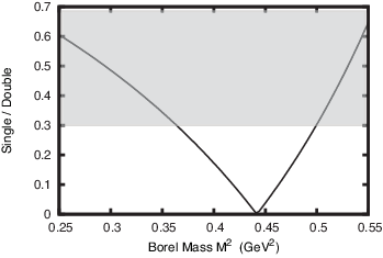
The choice of the Borel mass, , is, however, quite arbitrary, and deviation from the above result due to the different choice of the Borel mass should be taken into account as theoretical uncertainty. In Fig. 5, we plot the ratio of the single and double pole contributions as a function of . From this figure we find that the single pole contribution rapidly increases when the Borel mass is varied from . We here assume our sum rules to be valid within the region of the Borel mass in which the single pole contribution is less than of the double pole contribution. This assumption leads to GeV2, and in this region, takes the following values:
| (200) |
Here, the lower value corresponds to the upper limit of the Borel mass, and vice versa.
Next, we discuss the uncertainty of the OPE calculation. In this case, the truncation of the OPE leads to the uncertainty. Let us estimate it by evaluating the relative size of the higher-order contributions. Among them, the four-quark condensates such as are expected to yield sizable contributions, since they are free from loop suppression. On the assumption that these contributions vanish when one takes the quark masses to be zero, we expect that they are suppressed at least a factor of . Therefore, the uncertainty of the OPE calculation is estimated to be .
Taking the above discussion into account, we finally evaluate the neutron EDM with theoretical uncertainty as follows:
| (201) |
where the first uncertainty stems from the phenomenological calculation while the second one comes from the approximation in the OPE. We also include uncertainties originate from those in (See Eq. (193).), which is indicated by the third error in the above equation66 6 We approximate the error in as the r.m.s. of the statistical and systematic errors displayed in Eq. (193). . After all, it is found that there is almost factor of uncertainty in our sum rule calculation.
Let us compare the result with those obtained by using the values of calculated with the QCD sum rules. In Ref. [22], the authors adopt GeV3 for from the QCD sum rules derived for the nucleon mass. The for is equal to that for in the non-relativistic quark limit. In Ref. [25], it is shown that the neutron EDM prediction in the non-relativistic quark model with the SU(6) spin-flavor symmetry is derived in the QCD sum rules using the value of . By substituting the value into Eq. (199), one obtains . The “realistic” value of evaluated by the QCD sum rules in Ref. [24], GeV3, leads to a slightly larger result: . Thus, the overall factors of of these results are several times larger than that of our result.
For one’s convenience, we substitute the numerical values for the QCD parameters in Eq. (200). Here we take , , , and [18, 26]. Then, with those parameters the center values, we find
| (202) |
The contributions from and the quark CEDMs to may be changed furthermore by about , mainly due to the theoretical uncertainty of .
10 Under the Peccei-Quinn symmetry
It is known that induces too large neutron EDM, the strong CP problem. The Peccei-Quinn (PQ) symmetry is one of the solutions for the strong CP problem. If the PQ symmetry is introduced, vanishes dynamically. However, if the quark CEDMs are non-vanishing, a linear term is induced to the axion potential [27],
| (203) |
where is the topological susceptibility
| (204) |
and is calculated by
| (205) |
Minimizing the axion potential, an effective term is induced from the quark CEDM,
| (206) |
Taking the induced term into account, the neutron EDM in the presence of the PQ symmetry is estimated as
| (207) |
where
| (208) |
The contributions from the strange quark CEDM are cancelled in the presence of the PQ symmetry [15]. Again, we substitute the numerical values for the QCD parameters as presented in the previous section. The result is
| (209) |
11 Conclusion and discussion
We have studied the neutron EDM induced by the CP-violating interactions up to the dimension-five operators. In order to derive the relation between the CP-violating interactions and the neutron EDM, we have used the QCD sum rule technique. There are several phenomenological parameters to estimate the relation numerically. Pospelov and Ritz also analysed the neutron EDM using the QCD sum rules [14, 15] and they determined the low-energy constant within the framework in the QCD sum rules. On the other hand, we have extracted the parameter from lattice calculations. This approach allows us to reduce a theoretical uncertainty and leads to a conservative constraint on the CP violations. Our result is about 70 % smaller compared with the one obtained by Pospelov and Ritz. There still remains a sizable uncertainty resulting from the QCD sum rules itself due to a choice of the Borel mass scale. We have estimated the uncertainty from the Borel mass scale assuming that the single pole contribution is less than 30 % of the double pole contributions. This assumption leads to the theoretical error of about .
Finally, we briefly comment on the contribution of the CP-violating dimension-six operators. Among the dimension-six operators, the following operator, called Weinberg operator,
might be comparable to the quark EDM and CEDM contributions since they suffer from the chiral suppression. The other CP-violating dimension-six operators are effective four-quark operators of light quarks, which are negligible in the neutron EDM in typical high-energy models since the Wilson coefficients are suppressed by the quark masses77 7 If the CP-violating four-quark operators include heavy quarks, the CEDMs for the light quarks and the Weinberg operators are radiatively induced by integration of the heavy quarks as shown in Ref. [28].. In our QCD sum rule calculation it is found that the contribution from the Weinberg operator is and thus sub-dominant. There are a lot of discussions on the significance of the Weinberg operator [29], though no consensus has been reached yet.
Acknowledgments
One of the authors (JH) appreciates useful discussion with Yasumichi Aoki. This work is supported by Grant-in-Aid for Scientific research from the Ministry of Education, Science, Sports, and Culture (MEXT), Japan, No. 20244037, No. 20540252, No. 22244021 and No.23104011 (JH), and also by World Premier International Research Center Initiative (WPI Initiative), MEXT, Japan. The work of NN is supported by Research Fellowships of the Japan Society for the Promotion of Science for Young Scientists.
Appendix
In this Appendix, we list some techniques which we use to carry out the calculation.
Appendix A Quark condensates on the CP-violating background
In this section, we discuss the effects of the CP-violating interactions on the quark condensates as well as on the quark and gluon background fields. We begin by estimating it for the generic quark bi-linear condensate , with a constant matrix for which the quark bi-linear is an Hermitian operator. Then, by using the results obtained there, we derive the relations between the quark condensates and the background fields.
First, we evaluate the quark bi-linear on the CP-violating background. The contribution of the QCD term at the leading order is evaluated as [30]
| (213) |
Substituting Eq. (8) into the above expression, we obtain
| (214) |
with . The first term in the equation is calculated with the aid of the integration by parts:
| (215) | |||||
For the second term, we insert the intermediate states and keep only the contributions of the one-particle states of the pseudo Nambu-Goldstone bosons and :
| (216) |
where is the pion decay constant88 8 We use the PCAC relation for , (217) and a similar relation for . , and and denote the masses of and , respectively99 9 The effect of the - mixing is suppressed by a small factor of and we ignore it for brevity. . As a result, we obtain
| (218) |
Other contributions also may be evaluated through a similar procedure. For the contribution of the -mass terms,
| (219) |
while for the contribution of the quark CEDM terms,
| (220) |
Furthermore, it is found that the quark EDMs induce no contribution.
Taking all of the contributions into account, we obtain the CP-violating contribution to the quark condensates as
| (223) |
Here, the second equality comes from the conditions in Eq. (13). Thus, the choice of the quark mass phases in Eq. (15) reduces the contribution of the CP-violating interactions to the vacuum condensates into a quite simple expression.
Note that the CP-violating contribution to the quark condensates vanishes in the basis where the term is completely rotated out into the imaginary mass term. Thus, the choice of this basis, which is often adopted in the chiral Lagrangian approach, simplifies the calculation. In our paper, however, we remain in a general basis in order to display each contribution explicitly.
Next, we discuss the way of translating the quark and gluon background fields into their condensates. To begin with, we consider a single quark line . In this case, it is related with the quark condensate as follows:
| (224) |
Using the Fierz identity, the right-hand side of the expression leads to
These quark condensate terms are evaluated by conducting the short-distance expansion of the quark field in the Fock-Schwinger gauge as
| (242) |
We note that in this gauge one does not need to care about Wilson-line operators for the quark fields. (See Appendix C.)
In the case of CP-even vacuum, the Lorentz and CP invariance of vacuum tell us that
| (243) |
On the other hand, on an electromagnetic background, may have non-zero VEV proportional to the electromagnetic field strength . The electromagnetic field dependence for quark condensates is given as
| (244) |
where is called the quark condensate magnetic susceptibility [22]. Similar parametrization is used for the condensates including the gluon background field:
| (245) |
| (246) |
As in Ref. [22], we assume , and to be proportional to the quark charge:
| (247) |
This assumption corresponds to neglecting of the closed-loop contribution with gluon exchange.
Now let us consider the effect of the CP-violating interaction in Eq. (5) to the quark condensates. By using Eq. (223) and the expansion in Eq. (242), we evaluate each quark condensate on the CP-violating background as follows (with omitting the subscriptions and / for simplicity as long as it is not confusing):
| (248) |
| (249) |
| (254) |
where we use the classical equations of motion in the quark condensates and move the covariant derivatives with help of total derivative. The validity of this procedure is discussed in Appendix B. Furthermore,
| (259) |
and
| (262) |
Taking the above discussion into account and using the relation,
| (263) |
and
| (264) |
we finally obtain the expression for the single quark line as follows:
| (271) |
Lastly, we evaluate the interaction part of the quark and gluon background fields,
| (272) |
Again, we use the Fierz identity and the short-distance expansion of the quark field, and through a similar calculation, we find the following results:
| (275) |
Appendix B Equations of motion
Let us discuss the validity of using classical equations of motion for quark condensates. We investigate the following quantity:
| (276) |
where is a (-number) matrix. The subscript indicates that this quantity is evaluated in the vacuum. One may readily generalize the discussion here for the case with other CP-violating sources. The discussion presented in this section is based on Ref. [31].
First, we define the generating functional on the same background:
| (277) |
Here, the Lagrangian density is
| (278) |
The functional derivative of the generating function with respect to the function yields Eq. (276), that is,
| (279) |
Now we replace the integration variable with a new integration variable as
| (280) |
Since this step does not change the integral, then we obtain
| (281) |
where the inverse of the Jacobian comes from the transformation of the measure for the fermionic variable.
Next, we evaluate the Jacobian in the expression above. Since we are interested in the first order derivative of the generating function, we expand the Jacobian in and keep only terms linear in .
| (282) |
Using the identity
| (283) |
we readily obtain the Jacobian as
| (284) |
It is found that if the trace of the matrix is non-zero, the Jacobian yields a singular factor, while if it vanishes we need careful treatment for evaluating this term. So, in the following discussion, we divide into two types; one is the term proportional to the unit matrix and the other is the traceless part.
First, we consider the case . Using Eqs. (279), (281), and (284), we obtain the following equation:
| (285) |
Once you carry out the normal ordering for the composite operator , the singular factor in the right-hand side vanishes. Thus we conclude that after normal ordering,
| (286) |
when . This equation implies that we may use the equations of motion for quark condensates in this case.
Next, we shall turn to the traceless part. In this case the Jacobian in Eq. (284) is written in terms of the anomaly function defined as
| (287) |
With this function, Eq. (284) leads to
| (288) |
The usual analysis for the chiral anomaly tells us that the function in Eq. (287) does not vanish only for the case . Thus, if , Eq. (286) is satisfied. When , on the other hand, the function is evaluated as
| (289) |
From Eqs. (279), (281), and (288) we eventually find that
| (290) |
This expression is simplified via the axial current anomaly equation:
| (291) |
Then, Eq. (290) leads to
| (292) |
Therefore, we are not able to use the classical equations of motion for quark condensates in this case.
As a result, we find that
| (295) |
Also, its conjugate leads to
| (298) |
Before concluding the section, we add a comment on the condensate of the total derivative terms. As we have already conducted in Eq. (292), the Lorentz invariance of vacuum implies that condensates of the divergence of quark bi-linear always vanish, i.e.,
| (299) |
with a constant matrix which transforms as a vector under the Lorentz transformation, such as , , or so. On the other hand, the total derivative of the quark bi-linear is written as
| (300) |
Thus we find
| (301) |
Appendix C Wilson Line in Fock-Schwinger gauge
Quark fields are always accompanied by an appropriate Wilson-line operator in order to compensate the different gauge transformation property of the quark fields at different space-time points. In the Fock-Schwinger gauge, however, one may always choose a particular path which makes the Wilson-line operator equal to identity [32]. We show this statement in the following. The Wilson line is written as
| (302) |
where
| (303) |
and denotes path-ordering. This operator depends on the choice of the integration path. Here we take a path such that
| (304) |
Then,
| (305) |
In the Fock-Schwinger field, the gluon field is expanded as
| (306) |
Inserting this expression into Eq. (305), we readily find that all terms in the exponential vanish due to the antisymmetric property of the gluon field strength tensor. Therefore,
| (307) |
References
- [1] K. Nakamura et al. [Particle Data Group Collaboration], J. Phys. G G 37, 075021 (2010).
- [2] N. Cabibbo, Phys. Rev. Lett. 10, 531 (1963).
- [3] M. Kobayashi and T. Maskawa, Prog. Theor. Phys. 49, 652 (1973).
- [4] C. A. Baker, D. D. Doyle, P. Geltenbort, K. Green, M. G. D. van der Grinten, P. G. Harris, P. Iaydjiev and S. N. Ivanov et al., Phys. Rev. Lett. 97, 131801 (2006).
- [5] K. Bodek, S. .Kistryn, M. Kuzniak, J. Zejma, M. Burghoff, S. Knappe-Gruneberg, T. Sander-Thoemmes and A. Schnabel et al., arXiv:0806.4837 [nucl-ex].
- [6] D. H. Beck et al. [nEDM Collaboration], arXiv:1111.1273 [nucl-ex].
- [7] S. N. Balashov, K. Green, M. G. D. van der Grinten, P. G. Harris, H. Kraus, J. M. Pendlebury, D. B. Shiers and M. A. H. Tucker et al., arXiv:0709.2428 [hep-ex].
- [8]
Y. Arimoto et. al., [NOP Collaboration],
http://j-parc.jp/researcher/Hadron/
en/pac_1001/pdf/KEK_J-PARC-PAC2009-11.pdf - [9] Y. Masuda, Talk at UCN2010, April 2010, RCNP, Japan.
- [10] J. Hisano, M. Nagai and P. Paradisi, Phys. Lett. B 642, 510 (2006) ; Phys. Rev. D 78, 075019 (2008) ; Phys. Rev. D 80, 095014 (2009).
- [11]
E. Shintani, S. Aoki, N. Ishizuka, K. Kanaya, Y. Kikukawa, Y. Kuramashi, M. Okawa and Y. Tanigchi et al.,
Phys. Rev. D 72, 014504 (2005);
F. Berruto, T. Blum, K. Orginos and A. Soni, Phys. Rev. D 73, 054509 (2006);
E. Shintani, S. Aoki, N. Ishizuka, K. Kanaya, Y. Kikukawa, Y. Kuramashi, M. Okawa and A. Ukawa et al., Phys. Rev. D 75, 034507 (2007) ;
E. Shintani, S. Aoki and Y. Kuramashi, Phys. Rev. D 78 (2008) 014503;
S. Aoki, R. Horsley, T. Izubuchi, Y. Nakamura, D. Pleiter, P. E. L. Rakow, G. Schierholz and J. Zanotti, arXiv:0808.1428 [hep-lat]. - [12] M. A. Shifman, A. I. Vainshtein and V. I. Zakharov, Nucl. Phys. B 147, 385 (1979); Nucl. Phys. B 147, 448 (1979).
- [13]
A. Pich and E. de Rafael,
Nucl. Phys. B 367, 313 (1991);
J. Hisano and Y. Shimizu, Phys. Rev. D 70, 093001 (2004);
K. Ottnad, B. Kubis, U. G. Meissner and F. K. Guo, Phys. Lett. B 687, 42 (2010). - [14] M. Pospelov and A. Ritz, Phys. Rev. Lett. 83, 2526 (1999); Nucl. Phys. B 573, 177 (2000).
- [15] M. Pospelov and A. Ritz, Phys. Rev. D 63, 073015 (2001).
- [16] R. D. Peccei and H. R. Quinn, Phys. Rev. Lett. 38, 1440 (1977).
- [17] R. J. Crewther, P. Di Vecchia, G. Veneziano and E. Witten, Phys. Lett. B 88, 123 (1979) [Erratum-ibid. B 91, 487 (1980)].
- [18] V. M. Belyaev and B. L. Ioffe, Sov. Phys. JETP 56, 493 (1982) [Zh. Eksp. Teor. Fiz. 83, 876 (1982)].
- [19]
L. J. Reinders, H. Rubinstein and S. Yazaki,
Phys. Rept. 127, 1 (1985);
S. Narison, World Sci. Lect. Notes Phys. 26, 1 (1989);
M. A. Shifman, Prog. Theor. Phys. Suppl. 131, 1 (1998). - [20] S. Narison, Phys. Lett. B 666, 455 (2008) .
- [21] V. A. Novikov, M. A. Shifman, A. I. Vainshtein and V. I. Zakharov, Fortsch. Phys. 32, 585 (1984).
- [22] B. L. Ioffe and A. V. Smilga, Nucl. Phys. B 232, 109 (1984).
- [23] Y. Aoki et al. [RBC-UKQCD Collaboration], Phys. Rev. D 78, 054505 (2008).
- [24] D. B. Leinweber, Annals Phys. 254, 328 (1997).
- [25] M. Pospelov and A. Ritz, Annals Phys. 318, 119 (2005) .
- [26] I. I. Kogan and D. Wyler, Phys. Lett. B 274, 100 (1992).
- [27] I. I. Y. Bigi and N. G. Uraltsev, Sov. Phys. JETP 73, 198 (1991).
- [28] J. Hisano, K. Tsumura and M. J. S. Yang, arXiv:1205.2212 [hep-ph].
- [29] D. A. Demir, M. Pospelov and A. Ritz, Phys. Rev. D 67, 015007 (2003).
- [30] M. A. Shifman, A. I. Vainshtein and V. I. Zakharov, Nucl. Phys. B 166,493 (1980).
- [31] H. D. Politzer, Nucl. Phys. B 172, 349 (1980).
- [32] S. V. Mikhailov and A. V. Radyushkin, Phys. Rev. D 45, 1754 (1992).