Decode-and-Forward Based Differential Modulation for Cooperative Communication System with Unitary and Non-Unitary Constellations

The data received at the destination from the relay in the $n$-th time interval will be

$\displaystyle y_{r,d}[n]=h_{r,d}{v}_{r}[n]+e_{r,d}[n],$

(6)

where $h_{r,d}\sim\mathcal{CN}\left(0,\sigma^{2}_{r,d}\right)$ is the channel gain of the relay-destination link and $e_{r,d}[n]\sim\mathcal{CN}\left(0,N_{r,d}\right)$ is the AWGN noise. It is assumed that $h_{r,d}$ remains constant over at least two consecutive time intervals $n-1$ and $n$. From (1) and (6), we have

$\displaystyle y_{r,d}[n]=y_{r,d}[n-1]{x}_{r}[n]+e^{\prime}_{r,d}[n],$

(7)

where $e^{\prime}_{r,d}[n]=e_{r,d}[n]-e_{r,d}[n-1]{x}_{r}[n]$ is the zero mean AWGN noise with $2N_{r,d}$ variance. Depending upon the erroneous demodulation of the data of the source in the relay, the conditional p.d.f. of $y_{r,d}[n]$ can be written as

	$\displaystyle p_{y_{r,d}[n]}$	$\displaystyle\left(y|y_{r,d}[n-1],x[n]\right)$
		$\displaystyle=\left(1-\epsilon\right)p_{y_{r,d}[n]}\left(y|y_{r,d}[n-1],{x}_{r}[n]=x[n]\right)$
		$\displaystyle+\epsilon p_{y_{r,d}[n]}\left(y|y_{r,d}[n-1],{x}_{r}[n]\neq x[n]\right),$		(8)

where $\epsilon$ is the average probability of error of the source-relay link. It can be noticed from (7) that $p_{y_{r,d}[n]}\left(y|y_{r,d}[n-1],{x}_{r}[n]=x[n]\right)\sim\mathcal{CN}\left(y_{r,d}[n-1]x[n],2N_{r,d}\right)$. From (7) and [19, Section III], it can be seen that $p_{y_{r,d}[n]}\left(y|y_{r,d}[n-1],{x}_{r}[n]\neq x[n]\right)$ denotes the p.d.f. of a Gaussian mixture random variable. With this observation we have

		$\displaystyle p_{y_{r,d}[n]}\left(y|y_{r,d}[n-1],{x}_{r}[n]\neq x[n]\right)$
		$\displaystyle=\frac{1}{2\pi N_{r,d}(M-1)}\sum^{M}_{i=1,i\neq p}e^{-\frac{1}{2N_{r,d}}\left|y_{r,d}[n]-y_{r,d}[n-1]x_{i}\right|^{2}},$		(9)

where it is assumed that $x[n]=x_{p}$, $p\in\left\{1,2,...,M\right\}$, $x_{p}\in\mathcal{A}$, is the symbol transmitted by the source. By noticing that $y_{s,d}[n]\sim\mathcal{CN}\left(y_{s,d}[n-1]x[n],2N_{s,d}\right)$ and owing to independence of $y_{s,d}[n]$ and $y_{r,d}[n]$, an ML decoder can be obtained by maximizing the joint conditional p.d.f. of $y_{s,d}[n]$ and $y_{r,d}[n]$ as follows:

		$\displaystyle\hat{x}[n]=\text{arg}\;\;\underset{x\in\mathcal{A}}{\text{max}}\>\displaystyle\left\{\frac{1}{N_{s,d}}\text{Re}\left\{y^{*}_{s,d}[n]y_{s,d}[n-1]x\right\}\right.$
		$\displaystyle\left.+\text{ln}\left((1-\epsilon)e^{\frac{1}{N_{r,d}}\text{Re}\left\{y^{*}_{r,d}[n]y_{r,d}[n-1]x\right\}}\right.\right.$
		$\displaystyle\left.\left.+\frac{\epsilon}{M-1}\sum^{M}_{i=1,x_{i}\neq x}e^{\frac{1}{N_{r,d}}\text{Re}\left\{y^{*}_{r,d}[n]y_{r,d}[n-1]x_{i}\right\}}\right)\right\}.$		(10)

It can be seen from (10) that the proposed decoder requires the destination to possess knowledge of the average probability of error of the source-relay link $\epsilon$ which is a function of the average signal-to-noise ratio (SNR) of the source-relay link. The relay can estimate the average SNR of the source-relay link and feed forward it to the destination. The destination can calculate the value of $\epsilon$ by using the average SNR of the source-relay link and use it for the ML decoding. Since statistics of a channel vary slowly as compared to the instantaneous channel values, the destination requires less frequent updating of the average SNR value of the source-relay link. Further, (10) is applicable to the $M$-PSK constellation, whereas, the existing decoders of the differential cooperative system [14, 12] are applicable to binary signaling only. For $M=2$, (10) reduces to the existing ML decoder of the binary data [14, 12]. However, the proposed decoder is computationally complex. Therefore, it is desired to have a low complexity decoder of the DF based differential cooperative system, which can provide maximum possible diversity.

Let $y_{s,d}[n]=0,\forall n$, i.e., direct link between the source and the destination is absent, then a log-likelihood ratio (LLR) based symbol-wise decoder can be obtained from (8) and (9) as follows:

$\displaystyle\Lambda^{c}_{p,q}=\ln\left(\frac{a+g_{1}}{a+g_{2}}\right),$

(11)

where $p,q=1,2,...,M,x_{p},x_{q}\in\mathcal{A}$, $x_{p}\neq x_{q}$, $a=\frac{\epsilon}{M-1}\sum^{M}_{i=1\atop i\neq p,q}\displaystyle e^{\frac{1}{N_{r,d}}\text{Re}\left\{y^{*}_{r,d}[n]y_{r,d}[n-1]x_{i}\right\}}$, $g_{1}=(1-\epsilon)e^{\frac{1}{N_{r,d}}\text{Re}\left\{y^{*}_{r,d}[n]y_{r,d}[n-1]x_{p}\right\}}+\frac{\epsilon}{M-1}e^{\frac{1}{N_{r,d}}\text{Re}\left\{y^{*}_{r,d}[n]y_{r,d}[n-1]x_{q}\right\}}$, and $g_{2}=(1-\epsilon)e^{\frac{1}{N_{r,d}}\text{Re}\left\{y^{*}_{r,d}[n]y_{r,d}[n-1]x_{q}\right\}}+\frac{\epsilon}{M-1}\\ \times e^{\frac{1}{N_{r,d}}\text{Re}\left\{y^{*}_{r,d}[n]y_{r,d}[n-1]x_{p}\right\}}$. The LLR decoder of (11) is used as follows to decide about $x_{p}$ or $x_{q}$: $\Lambda^{c}_{p,q}\overset{x_{p}}{\underset{x_{q}}{\gtrless}}0$. Since $a,g_{1},g_{2}\geq 0$, it can be shown after some simple algebra that the decision rule $\ln\left(\frac{a+g_{1}}{a+g_{2}}\right)\overset{x_{p}}{\underset{x_{q}}{\gtrless}}0$ is the same as $\ln\left(\frac{g_{1}}{g_{2}}\right)\overset{x_{p}}{\underset{x_{q}}{\gtrless}}0$.

Hence, we have the following LLR decoder from (11):

$\displaystyle\Lambda^{c}_{p,q}=f(t)=\text{ln}\left(\frac{(1-\epsilon)e^{t}+\frac{\epsilon}{M-1}}{(1-\epsilon)+\frac{\epsilon}{M-1}e^{t}}\right),$

(12)

where $t=\frac{1}{N_{r,d}}\text{Re}\left\{y^{*}_{r,d}[n]y_{r,d}[n-1]\left(x_{p}-x_{q}\right)\right\}$. It can be seen from (12) that $f(t)$ clipps to $T=\pm\text{ln}\left((M-1)(1-\epsilon)/\epsilon\right)$ for very large and very small values of $t$. Further, it is shown in Table I and Fig. 2 for 16-PSK constellation that we can approximate $f(t)$ by a piecewise linear function as follows:

$\displaystyle f(t)\approx f_{\text{PL}}(t)\triangleq\left\{\begin{array}[]{ccc}-T,&\text{if}&t<-T,\\ t,&\text{if}&-T\leq t\leq T,\\ T,&\text{if}&t>T.\end{array}\right.$

From (10) and (III-B), we get the following suboptimal PL decoder in the destination if the direct link between the source and destination is present:

$\displaystyle\Lambda_{p,q}\approx t_{0}+f_{\text{PL}}(t),$

(16)

where $t_{0}=\frac{1}{N_{s,d}}\text{Re}\left\{y^{*}_{s,d}[n]y_{s,d}[n-1]\left(x_{p}-x_{q}\right)\right\}$. The proposed PL decoder is applied in a pair-wise manner to the constellation points for taking a decision of the symbol transmitted by the source. For example, for QPSK constellation containing the following four signal points: $x_{1},x_{2},x_{3},x_{4}$, the proposed PL decoder decides that $x_{k},k=1,2,3,4,$ is the transmitted symbol if $\Lambda_{k,l}>0,\forall l\in\left\{1,2,3,4\right\},k\neq l$, where $\Lambda_{k,l}$ is calculated from (16).

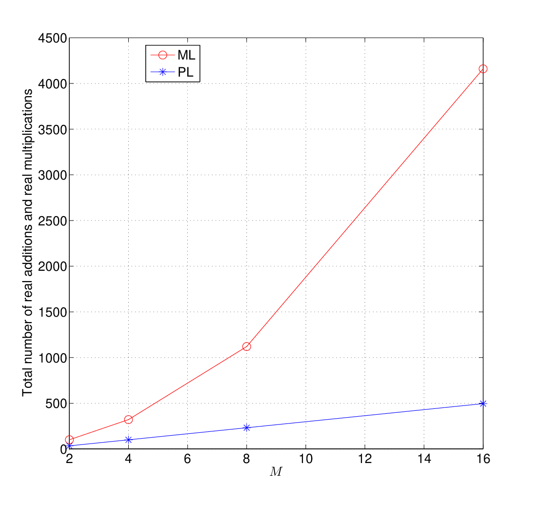
The total number of the real additions and real multiplications required by the proposed ML decoder (10) and the proposed PL decoder (16) for decoding a symbol belonging to the $M$-PSK, $M\geq 2$, constellation can be obtained after some manipulations as $15M^{2}+20M$ and $33(M-1)$, respectively. We have plotted the decoding complexity (the total number of the real additions and real multiplications) of the proposed ML and PL decoders for different $M$-PSK constellations in Fig. 3. It can be seen from Fig. 3 that the decoding complexity of the proposed PL decoder increases linearly, whereas, the decoding complexity of the proposed ML decoder increases exponentially with the size of the $M$-PSK constellation. Moreover, the proposed PL decoder significantly reduces the computational effort as compared to the proposed ML decoder for $M\geq 4$.

The non-unitary constellations like $M$-QAM are useful for increasing the data rate and coding gain as compared to the $M$-PSK constellation in communication systems. Therefore, treatment of the differential modulation based cooperative communication system with non-unitary constellation is imperative. For non-unitary constellation like $M$-QAM, $|x[n]|^{2}$ is not necessarily equal to unity, therefore, we need to modify (1) to satisfy the average power constraint as

$\displaystyle v[n]=v[n-1]\frac{x[n]}{\left|x[n-1]\right|},$

(17)

where $\left|\cdot\right|$ denotes the absolute value. From (3) and (17), we have

$\displaystyle y_{s,r}[n]=y_{s,r}[n-1]\frac{x[n]}{\left|x[n-1]\right|}+e^{\prime}_{s,r}[n],$

(18)

where $e^{\prime}_{s,r}[n]=e_{s,r}[n]-e_{s,r}[n-1]\frac{x[n]}{\left|x[n-1]\right|}\sim\mathcal{CN}\left(0,(1+\frac{\left|x[n]\right|^{2}}{\left|x[n-1]\right|^{2}})N_{s,r}\right)$. As $y_{s,r}[n]\!\!\sim\!\mathcal{CN}\!\left(\!y_{s,r}[n-1]\frac{x[n]}{\left|x[n-1]\right|},(1\!+\!\frac{\left|x[n]\right|^{2}}{\left|x[n-1]\right|^{2}})N_{s,r}\!\right)$, therefore, the relay demodulates $x[n]$ as

		$\displaystyle{x}_{r}[n]=\text{arg}\;\;\underset{x\in\mathcal{\chi}}{\text{min}}\left\{\text{ln}\left(1+\frac{|x|^{2}}{\left|x[n-1]\right|^{2}}\right)+\frac{1/N_{s,r}}{1+\frac{|x|^{2}}{\left|x[n-1]\right|^{2}}}\right.$
		$\displaystyle\left.\hskip 50.00008pt\times\left|y_{s,r}[n]-y_{s,r}[n-1]\frac{x}{\left|x[n-1]\right|}\right|^{2}\right\},$		(19)

where $\mathcal{\chi}$ is an $M$-QAM constellation. It can be seen from (19) that the differential decoder assumes that $x[n-1]$ is perfectly known to the receiver. Since it is not possible for the receiver to have perfect knowledge of $x[n-1]$, the differential decoder of (19) can utilize an estimate of $x[n-1]$.

From (2), (6), and (17), we can write

	$\displaystyle y_{s,d}[n]$	$\displaystyle=y_{s,d}[n-1]\frac{x[n]}{\left|x[n-1]\right|}+e^{\prime}_{s,d}[n],$
	$\displaystyle y_{r,d}[n]$	$\displaystyle=y_{r,d}[n-1]\frac{{x}_{r}[n]}{\left|x_{r}[n-1]\right|}+e^{\prime}_{r,d}[n],$		(20)

where $e^{\prime}_{s,d}[n]=e_{s,d}[n]-e_{s,d}[n-1]\frac{x[n]}{\left|x[n-1]\right|}\sim\mathcal{CN}\left(0,(1+|x[n]|^{2}/\left|x[n-1]\right|^{2})N_{s,d}\right)$ and $e^{\prime}_{r,d}[n]=e_{r,d}[n]-e_{r,d}[n-1]\frac{{x}_{r}[n]}{\left|x_{r}[n-1]\right|}$ $\sim\mathcal{CN}\left(0,(1+|{x}_{r}[n]|^{2}/\left|x_{r}[n-1]\right|^{2})N_{r,d}\right)$. The joint conditional p.d.f. of $y_{s,d}[n]$ and $y_{r,d}[n]$ can be maximized to obtain the following ML decoder of the differential $M$-QAM data:

		$\displaystyle\hat{x}[n]=\text{arg}\;\;\underset{x\in\chi}{\text{max}}\>\left\{-\text{ln}\left(1+\frac{|x|^{2}}{\left|x[n-1]\right|^{2}}\right)\right.$
		$\displaystyle\left.-\frac{\left|y_{s,d}[n]-y_{s,d}[n-1]\frac{x}{\left|x[n-1]\right|}\right|^{2}}{\left(1+\frac{|x|^{2}}{\left|x[n-1]\right|^{2}}\right)N_{s,d}}\right.$
		$\displaystyle\left.+\text{ln}\left(\frac{(1-\epsilon)}{1+\frac{|x|^{2}}{\left|{x}_{r}[n-1]\right|^{2}}}e^{-\frac{\left|y_{r,d}[n]-y_{r,d}[n-1]\frac{x}{\left|{x}_{r}[n-1]\right|}\right|^{2}}{\left(1+\frac{|x|^{2}}{\left|{x}_{r}[n-1]\right|^{2}}\right)N_{r,d}}}+\frac{\epsilon}{M-1}\right.\right.$
		$\displaystyle\left.\left.\times\sum^{M}_{i=1\atop x_{i}\neq x}\frac{1}{1+\frac{|x_{i}|^{2}}{\left|{x}_{r}[n-1]\right|^{2}}}e^{-\frac{\left|y_{r,d}[n]-y_{r,d}[n-1]\frac{x_{i}}{\left|{x}_{r}[n-1]\right|}\right|^{2}}{\left(1+\frac{|x_{i}|^{2}}{\left|{x}_{r}[n-1]\right|^{2}}\right)N_{r,d}}}\right)\right\}.$		(21)

Since the destination does not have perfect knowledge of $x[n-1]$ and ${x}_{r}[n-1]$, it can utilize the estimated values of $x[n-1]$ and ${x}_{r}[n-1]$ in (21) for decoding the currently transmitted data of the source. The estimate of ${x}_{r}[n-1]$ in the destination can be obtained by using the following differential decoder:

	$\displaystyle\hat{{x}}_{r}[n-1]=\text{arg}\!\!\;\;\underset{x\in\mathcal{\chi}}{\text{min}}$	$\displaystyle\!\left\{\frac{\left|y_{r,d}[n-1]-y_{r,d}[n-2]\frac{x}{\left|{x}_{r}[n-2]\right|}\right|^{2}}{\left(1+\frac{|x|^{2}}{\left|{x}_{r}[n-2]\right|^{2}}\right)N_{r,d}}\right.$
		$\displaystyle\left.+\text{ln}\left(\!1\!+\!\frac{|x|^{2}}{\left|{x}_{r}[n-2]\right|^{2}}\right)\!\!\right\}.$		(22)

It will be shown in Subsection VI-A through Fig. 6 that use of the estimated value of $x[n-1]$ in the relays and estimated values of $x[n-1]$ and ${x}_{r}[n-1]$ in the destination does not lead to error propagation in the performance of the destination receiver for different $M$-QAM constellations.

After some algebra, the PL decoder of the differential $M$-QAM data can be obtained as follows:

$\displaystyle\Lambda_{p,q}\approx u_{0}+f_{\text{PL}}(u_{r}),$

(23)

where

	$\displaystyle u_{0}=$	$\displaystyle\ln\left(\frac{\left|x[n-1]\right|^{2}+\left|x_{q}\right|^{2}}{\left|x[n-1]\right|^{2}+\left|x_{p}\right|^{2}}\right)$
		$\displaystyle\hskip 0.0pt+\frac{\left|y_{s,d}[n]-y_{s,d}[n-1]\frac{x_{q}}{\left|x[n-1]\right|}\right|^{2}}{\left(1+\left|x_{q}\right|^{2}/\left|x[n-1]\right|^{2}\right)N_{s,d}}$
		$\displaystyle\hskip 0.0pt-\frac{\left|y_{s,d}[n]-y_{s,d}[n-1]\frac{x_{p}}{\left|x[n-1]\right|}\right|^{2}}{\left(1+\left|x_{p}\right|^{2}/\left|x[n-1]\right|^{2}\right)N_{s,d}},$
	$\displaystyle u_{r}=$	$\displaystyle\ln\left(\frac{\left|{x}_{r}[n-1]\right|^{2}+\left|x_{q}\right|^{2}}{\left|{x}_{r}[n-1]\right|^{2}+\left|x_{p}\right|^{2}}\right)$
		$\displaystyle+\frac{\left|y_{r,d}[n]-y_{r,d}[n-1]\frac{x_{q}}{\left|{x}_{r}[n-1]\right|}\right|^{2}}{\left(1+{|x_{q}|^{2}}/{\left|{x}_{r}[n-1]\right|^{2}}\right)N_{r,d}}$
		$\displaystyle-\frac{\left|y_{r,d}[n]-y_{r,d}[n-1]\frac{x_{p}}{\left|{x}_{r}[n-1]\right|}\right|^{2}}{\left(1+{|x_{p}|^{2}}/{\left|{x}_{r}[n-1]\right|^{2}}\right)N_{r,d}},$		(24)

and $f_{\text{PL}}(u_{r})$ is given in (III-B). The proposed PL decoder of the $M$-QAM constellation given in (23) provides decoding complexity which is linear in $M$. Therefore, the proposed PL decoder of the $M$-QAM constellation also reduces the decoding complexity as compared to the proposed ML decoder (21).

Remark: We utilize one-way relaying in this paper for simplicity. The ML and PL decoders obtained in this paper can be extended to the two-way relaying based differential DF system. However, the extension can be more involved.

Let $x[n]=x_{p}$, $x_{p}\in\mathcal{A}$, be the $M$-PSK symbol transmitted by the source and the destination wrongly decides that $\hat{x}[n]=x_{q}$, $x_{q}\in\mathcal{A}$, is the transmitted $M$-PSK symbol. The probability of error of the destination receiver can be expressed in terms of three mutually exclusive events. The conditional uncoded pairwise error probability (PEP), given that the channel gains of the source-destination and relay-destination links are known in the destination, is

		$\displaystyle P^{x_{p},x_{q}}_{e}(h_{s,d},h_{r,d})$
		$\displaystyle=\text{Pr}\left\{t_{0}-T<0|t<-T,x[n]\!\!=\!\!x_{p}\right\}\text{Pr}\left\{t<-T|x[n]\!\!=\!\!x_{p}\right\}$
		$\displaystyle+\text{Pr}\left\{t_{0}+T<0|t>T,x[n]=x_{p}\right\}\text{Pr}\left\{t>T|x[n]=x_{p}\right\}$
		$\displaystyle+\text{Pr}\left\{t_{0}+t<0,-T\leq t\leq T|x[n]=x_{p}\right\},$		(25)

where $\text{Pr}\left\{\cdot\right\}$ represents the probability of an event. Let $\gamma_{s,d}=|h_{s,d}|^{2}/N_{s,d}$ and $\gamma_{r,d}=|h_{r,d}|^{2}/N_{r,d}$ be the instantaneous SNR of the source-destination and relay-destination link, respectively. It is shown in Appendix A that the conditional uncoded PEP of the PL decoder in a differential cooperative system utilizing the DF protocol when $h_{s,d}$ and $h_{r,d}$ are known in the destination, will be

		$\displaystyle P^{x_{p},x_{q}}_{e}(h_{s,d},h_{r,d})=P_{e_{1}}(h_{s,d})\left(P_{e_{2}}(h_{r,d})+P_{e_{3}}(h_{r,d})\right)$
		$\displaystyle+P_{e_{4}}(h_{s,d})\left(P_{e_{5}}(h_{r,d})+P_{e_{6}}(h_{r,d})\right)+P_{e_{7}}(h_{s,d},h_{r,d})$
		$\displaystyle+P_{e_{8}}(h_{s,d},h_{r,d})+P_{e_{9}}(h_{s,d},h_{r,d})+P_{e_{10}}(h_{s,d},h_{r,d}),$		(26)

where the terms $P_{e_{i}}\left(\cdot\right),i=1,2,..,6$ and $P_{e_{j}}\left(\cdot,\cdot\right),j=7,..,10$ are given in Appendix A.

If $h_{s,d}$ and $h_{r,d}$ are the complex-valued Gaussian random variables, then $\gamma_{s,d}$ and $\gamma_{r,d}$ will be Xi-square distributed with the following p.d.f.s [20]:

	$\displaystyle p_{\gamma_{s,d}}(\gamma)$	$\displaystyle=\frac{1}{\bar{\gamma}_{s,d}}e^{-\frac{\gamma}{\bar{\gamma}_{s,d}}}$
	$\displaystyle p_{\gamma_{r,d}}(\gamma)$	$\displaystyle=\frac{1}{\bar{\gamma}_{r,d}}e^{-\frac{\gamma}{\bar{\gamma}_{r,d}}},$		(27)

where $\bar{\gamma}_{s,d}=\sigma^{2}_{s,d}/N_{r,d}$ and $\bar{\gamma}_{r,d}=\sigma^{2}_{r,d}/N_{r,d}$ are the average SNRs of the source-destination and relay-destination links, respectively. The average uncoded PEP of decoding $x_{q}$ in place of $x_{p}$ can be obtained as

		$\displaystyle P^{x_{p},x_{q}}_{e}=E\left\{P^{x_{p},x_{q}}_{e}(h_{s,d},h_{r,d})\right\}$
		$\displaystyle=\int^{\infty}_{0}\int^{\infty}_{0}P^{x_{p},x_{q}}_{e}(\gamma_{1},\gamma_{2})p_{\gamma_{s,d}}(\gamma_{1})p_{\gamma_{r,d}}(\gamma_{2})d\gamma_{1}\>d\gamma_{2},$		(28)

where $E\left\{\cdot\right\}$ denotes the expectation. It is shown in Appendix A that the closed-form average PEP of decoding $x_{q}$ in place of $x_{p}$ in the DF based differential cooperative system using the $M$-PSK constellation will be

	$\displaystyle P^{x_{p},x_{q}}_{e}=$	$\displaystyle P_{e_{1}}(P_{e_{2}}+P_{e_{3}})+P_{e_{4}}(P_{e_{5}}+P_{e_{6}})+P_{e_{7}}+P_{e_{8}}$
		$\displaystyle+P_{e_{9}}+P_{e_{10}},$		(29)

where the terms $P_{e_{l}},l=1,2,..,10$ are given in Appendix A.

The constellation diagram of an arbitrary $M$-PSK constellation is shown in Fig.​ 4. The decision boundaries corresponding to the symbol $x_{1}$ are also shown. From equiprobability of the constellation points it can be deduced that

$\displaystyle\text{Pr}\left[\text{error}\right]=\frac{1}{M}\sum^{M}_{i=1}\text{Pr}\left[\text{error}|x_{i}\right]=\text{Pr}\left[\text{error}|x_{1}\right].$

(30)

Let $x_{p}=x_{1}=1$ is the transmitted symbol, then the SER of the $M$-PSK constellation can be approximated by using the nearest neighbors approach [21, Subsection 5.1.5] as

$\displaystyle P_{e}\approx P^{x_{2},1}_{e}+P^{x_{M},1}_{e},$

(31)

where $P^{x_{2},1}_{e}$ and $P^{x_{M},1}_{e}$ are the average probabilities of error of decoding $x_{2}$ and $x_{M}$, respectively, in place of the originally transmitted symbol $x_{1}=1$. We can calculate $P^{x_{2},1}_{e}$ and $P^{x_{M},1}_{e}$ by using (29).

Expression of the SER of the PL decoder given in (29) and (31) is very complicated and it is difficult to draw a conclusion from it. Therefore, we will derive an approximate SER of the proposed PL decoder with $M$-PSK constellation by ignoring the higher order noise in this subsection. For simplicity, we assume that $x_{q}$ is the transmitted symbol and the destination wrongly decides that $x_{p}$ was transmitted. It can be noticed that because of symmetry of the $M$-PSK constellation $P^{x_{p},x_{q}}_{e}=P^{x_{q},x_{p}}_{e}$. By ignoring the higher order noise terms in $t_{0}$ and $t$, it can be shown after some manipulations that $t_{0}\sim\mathcal{N}\left(\text{Re}\left\{\gamma_{s,d}x^{*}_{q}\bar{x}\right\},\gamma_{s,d}\left|\bar{x}\right|^{2}\right)$ and $t\sim\mathcal{N}\left(\text{Re}\left\{\gamma_{r,d}{x}^{*}_{r}\bar{x}\right\},\gamma_{r,d}\left|\bar{x}\right|^{2}\right)$, where $\bar{x}=x_{p}-x_{q}$ and $x_{r}$ is the symbol transmitted by the relay. After many algebraic manipulations, the average pairwise error probability of the proposed PL decoder can be obtained by ignoring the higher order noise as

$\displaystyle P^{x_{p},x_{q}}_{e}\approx I_{1}(\bar{\gamma},T)+I_{2}(\bar{\gamma},T)+I_{3}(\bar{\gamma},T)+I_{4}(\bar{\gamma},T),$

(32)

where

		$\displaystyle I_{1}(\bar{\gamma},T)=(1-\epsilon)\frac{1}{\bar{\gamma}_{s,d}}\int^{\infty}_{0}Q\left(\frac{T-z_{q}\gamma_{s,d}}{\left|\bar{x}\right|\sqrt{\gamma_{s,d}}}\right)e^{-\frac{\gamma_{s,d}}{\bar{\gamma}_{s,d}}}d\gamma_{s,d}$
		$\displaystyle\times\frac{1}{\bar{\gamma}_{r,d}}\int^{\infty}_{0}Q\left(\frac{T+z_{q}\gamma_{r,d}}{\left|\bar{x}\right|\sqrt{\gamma_{r,d}}}\right)e^{-\frac{\gamma_{r,d}}{\bar{\gamma}_{r,d}}}d\gamma_{r,d}$
		$\displaystyle+\frac{\epsilon}{M-1}\frac{1}{\bar{\gamma}_{s,d}}\int^{\infty}_{0}Q\left(\frac{T-z_{q}\gamma_{s,d}}{\left|\bar{x}\right|\sqrt{\gamma_{s,d}}}\right)e^{-\frac{\gamma_{s,d}}{\bar{\gamma}_{s,d}}}d\gamma_{s,d}$
		$\displaystyle\times\sum^{M}_{i=1\atop i\neq q}\left(\frac{1}{\bar{\gamma}_{r,d}}\int^{\infty}_{0}Q\left(\frac{T+z_{i}\gamma_{r,d}}{\left|\bar{x}\right|\sqrt{\gamma_{r,d}}}\right)e^{-\frac{\gamma_{r,d}}{\bar{\gamma}_{r,d}}}d\gamma_{r,d}\right),$
		$\displaystyle I_{2}(\bar{\gamma},T)=(1-\epsilon)\frac{1}{\bar{\gamma}_{s,d}}\int^{\infty}_{0}Q\left(\frac{-T-z_{q}\gamma_{s,d}}{\left|\bar{x}\right|\sqrt{\gamma_{s,d}}}\right)e^{-\frac{\gamma_{s,d}}{\bar{\gamma}_{s,d}}}d\gamma_{s,d}$
		$\displaystyle\times\frac{1}{\bar{\gamma}_{r,d}}\int^{\infty}_{0}Q\left(\frac{T-z_{q}\gamma_{r,d}}{\left|\bar{x}\right|\sqrt{\gamma_{r,d}}}\right)e^{-\frac{\gamma_{r,d}}{\bar{\gamma}_{r,d}}}d\gamma_{r,d}$
		$\displaystyle+\frac{\epsilon}{M-1}\frac{1}{\bar{\gamma}_{s,d}}\int^{\infty}_{0}Q\left(\frac{-T-z_{q}\gamma_{s,d}}{\left|\bar{x}\right|\sqrt{\gamma_{s,d}}}\right)e^{-\frac{\gamma_{s,d}}{\bar{\gamma}_{s,d}}}d\gamma_{s,d}$
		$\displaystyle\times\sum^{M}_{i=1\atop i\neq q}\left(\frac{1}{\bar{\gamma}_{r,d}}\int^{\infty}_{0}Q\left(\frac{T-z_{i}\gamma_{r,d}}{\left|\bar{x}\right|\sqrt{\gamma_{r,d}}}\right)e^{-\frac{\gamma_{r,d}}{\bar{\gamma}_{r,d}}}d\gamma_{r,d}\right),$
		$\displaystyle I_{3}(\bar{\gamma},T)=\frac{1-\epsilon}{\bar{\gamma}_{s,d}\bar{\gamma}_{r,d}}\int^{\infty}_{\gamma_{s,d}=0}\int^{\infty}_{\gamma_{r,d}=0}\frac{1}{\sqrt{2\pi\gamma_{r,d}}\left|\bar{x}\right|}$
		$\displaystyle\times\int^{T}_{-T}e^{-\frac{1}{2}\frac{\left(w-z_{q}\gamma_{r,d}\right)^{2}}{\left|\bar{x}\right|^{2}{\gamma_{r,d}}}}Q\left(\frac{-w-z_{q}\gamma_{s,d}}{\left|\bar{x}\right|\sqrt{\gamma_{s,d}}}\right)e^{-\frac{\gamma_{s,d}}{\bar{\gamma}_{s,d}}}$
		$\displaystyle\times e^{-\frac{\gamma_{r,d}}{\bar{\gamma}_{r,d}}}dwd\gamma_{r,d}d\gamma_{s,d},$
		$\displaystyle I_{4}(\bar{\gamma},T)=\frac{\epsilon}{\bar{\gamma}_{s,d}\bar{\gamma}_{r,d}}\int^{\infty}_{\gamma_{s,d}=0}\int^{\infty}_{\gamma_{r,d}=0}\frac{1}{\sqrt{2\pi\gamma_{r,d}}\left|\bar{x}\right|(M-1)}$
		$\displaystyle\times\int^{T}_{-T}Q\left(\frac{-w-z_{q}\gamma_{s,d}}{\left|\bar{x}\right|\sqrt{\gamma_{s,d}}}\right)\sum^{M}_{i=1\atop i\neq q}e^{-\frac{1}{2}\frac{\left(w-z_{i}\gamma_{r,d}\right)^{2}}{\left|\bar{x}\right|^{2}{\gamma_{r,d}}}}e^{-\frac{\gamma_{s,d}}{\bar{\gamma}_{s,d}}}$
		$\displaystyle\times e^{-\frac{\gamma_{r,d}}{\bar{\gamma}_{r,d}}}dwd\gamma_{r,d}d\gamma_{s,d},$		(33)

where $Q\left(\cdot\right)$ is the Q-function [22, Eq. (2.3.10)], $z_{q}=\text{Re}\left\{x_{q}\bar{x}^{*}\right\}$, and $z_{i}=\text{Re}\left\{x_{i}\bar{x}^{*}\right\}$. It is difficult to solve the integration in (32) analytically, therefore, the approximate average SER of the PL decoder can be obtained numerically from (31) and (32). We can use (32) for analytically finding the diversity of the PL decoder.

References

• [1] S. M. Alamouti, “A simple transmit diversity technique for wireless communications,” IEEE J. Select. Areas Commun., vol. 16, no. 8, pp. 1451–1458, Oct. 1998.
• [2] V. Tarokh and H. Jafarkhani, “A differential detection scheme for transmit diversity,” IEEE J. Select. Areas Commun., vol. 18, no. 7, pp. 1169–1174, Jul. 2000.
• [3] A. Sendonaris, E. Erkip, and B. Aazhang, “User cooperation diversity — Part I: System description,” IEEE Trans. Commun., vol. 51, no. 11, pp. 1927–1938, Nov. 2003.
• [4] A. Nosratinia, T. E. Hunter, and A. Hedayat, “Cooperative communication in wireless networks,” IEEE Commun. Mag., vol. 42, no. 10, pp. 74–80, Oct. 2004.
• [5] J. N. Laneman, D. N. C. Tse, and G. W. Wornell, “Cooperative diversity in wireless networks: Efficient protocols and outage behaviour,” IEEE Trans. Inform. Theory, vol. 50, no. 12, pp. 389–400, Dec. 2004.
• [6] J. N. Laneman and G. W. Wornell, “Distributed space-time-coded protocols for exploiting cooperative diversity in wireless networks,” IEEE Trans. Inform. Theory, vol. 49, no. 10, pp. 2415–2425, Oct. 2003.
• [7] Y. Jing and B. Hassibi, “Distributed space-time coding in wireless relay networks,” IEEE Trans. Wireless Commun., vol. 5, no. 12, pp. 3524–3536, Dec. 2006.
• [8] Y. Jing and H. Jafarkhani, “Using orthogonal and quasi-orthogonal designs in wireless relay networks,” IEEE Trans. Inform. Theory, vol. 53, no. 11, pp. 4106–4118, Nov. 2007.
• [9] L. Song, Y. Li, A. Huang, B. Jiao, and A. V. Vasilakos, “Differential modulation for bidirectional relaying with analog network coding,” IEEE Trans. Signal Process., vol. 58, pp. 3933–3938, Jul. 2010.
• [10] Q. Zhao and H. Li, “Performance of differential modulation with wireless relays in Rayleigh fading channels,” IEEE Commun. Lett., vol. 9, no. 4, pp. 343–345, Apr. 2005.
• [11] ——, “Performance analysis of an amplify-based differential modulation for wireless relay networks under Nakagami-m fading channels,” Proc. IEEE Int. Workshop on Signal Process. Advances in Wireless Communications, pp. 211–215, Jun. 2005, New York, USA.
• [12] ——, “Differential modulation for cooperative wireless system,” IEEE Trans. Signal Process., vol. 55, no. 5, pp. 2273–2283, May 2007.
• [13] T. Himsoon, W. Su, and K. J. R. Liu, “Differential transmission for amplify-and-forward cooperative communications,” IEEE Signal Process. Lett., vol. 12, no. 9, pp. 597–600, Sep. 2006.
• [14] D. Chen and J. N. Laneman, “Modulation and demodulation for cooperative diversity in wireless systems,” IEEE Trans. Wireless Commun., vol. 5, no. 7, pp. 1785–1794, July 2006.
• [15] Z. Fang, L. Li, X. Bao, and Z. Wang, “Generalized differential modulation for amplify-and-forward wireless relay networks,” IEEE Trans. Vehicular Technol., vol. 58, no. 6, pp. 3058–3062, July 2009.
• [16] Q. Zhao and H. Li, “Performance of decode-based differential modulation for wireless relay networks in Nakagami-m channels,” in Proc. 2006 IEEE Int. Conf. Acoustics, Speech, Signal Processing, pp. 673–675, May 2006, Toulouse, France.
• [17] Q. Zhao, H. Li, and P. Wang, “Performance of cooperative relay with binary modulation in Nakagami-m fading channels,” IEEE Trans. Vehicular Technol., vol. 57, no. 5, pp. 3310–3315, Sep. 2008.
• [18] T. Cui, F. Gao, and C. Tellambura, “Differential modulation for two-way wireless communications: A perspective of differential network coding at the physical layer,” IEEE Trans. Commun., vol. 57, no. 10, pp. 2977–2987, Oct. 2009.
• [19] L. Trailovic and L. Y. Pao, “Variance estimation and ranking of target tracking position errors modeled using Gaussian mixture distributions,” Automatica, vol. 41, no. 8, pp. 1433–1438, Aug. 2005.
• [20] J. G. Proakis, Digital Communications, 4th ed. Singapore: McGraw-Hill, 2001.
• [21] A. Goldsmith, Wireless Communications, 1st ed. Cambridge, UK: Cambridge Univ. Press, 2005.
• [22] J. G. Proakis and M. Salehi, Digital Communications, 5th ed. New York, USA: McGraw-Hill Book Company, 2008.
• [23] M. K. Simon and M.-S. Alouini, Digital Communication over Fading Channels. New Jersey, USA: John Wiley & Sons, Inc., 2005.
• [24] I. S. Gradshteyn and I. M. Ryzhik, Table of Integrals, Series, and Products, 6th ed. San Diego, CA, USA: Academic Press, 2000.
• [25] M. Abramowitz and I. A. Stegun, Handbook of Mathematical Functions. New York, USA: Dover Publications, Inc., 1972.
• [26] K. H. Biyari and W. C. Lindsey, “Statistical distributions of hermitian quadratic forms in complex Gaussian variables,” IEEE Trans. Inform. Theory, vol. 39, no. 3, pp. 1076–1082, May 1993.
• [27] E. G. Larsson and P. Stoica, Space-Time Block Coding for Wireless Communications. Cambridge, UK: Cambridge University Press, 2003.