A supersymmetric holographic dual of a fractional topological insulator
Martin Ammon and Michael Gutperle
Department of Physics and Astronomy
University of California, Los Angeles, CA 90095, USA
ammon, gutperle@physics.ucla.edu;
Abstract
We construct a supersymmetric generalization of the holographic dual of a fractional topological insulator found in [1]. This is accomplished by introducing a nontrivial gauge field on the world volume of the probe D7 brane. The BPS equations are derived from the -symmetry transformation of the probe brane. The BPS equations are shown to reduce to two first oder nonlinear partial differential equations. Solutions of the BPS equations correspond to a probe brane configuration which preserves four of the thirty-two supersymmetries of the background. Solutions of the BPS equations which correspond to a holographic fractional topological insulator are obtained numerically.
1 Introduction
The AdS/CFT correspondence, and more generally gauge/gravity dualities, provide a powerful tool for studying strongly coupled field theories in states with finite density, and hence might be useful in condensed matter physics (see [2, 3, 4] and references therein). For example, superfluids [5, 6, 7] and Non-Fermi liquids [8] can be realized in bottom-up models within this framework. Note that such bottom-up models are generically formulated in terms of four or five dimensional gravity theories coupled to scalars and gauge fields. It might or might not be possible to embed such models into string theory. Consequently, the dual field theory formulation in terms of elementary fields and a Lagrangian is in general not known or might even not exist. String theory embeddings of these bottom-up models can be realized by using probe branes in the background of D3–branes. In this case the dual field theory is known explicitly. For example p-wave superfluids [9, 10, 11], Fermi surfaces [12] and the gravity dual of a Quantum Hall Plateau transition [13] were investigated.
In this paper we consider the dual gravity description of a fractional topological insulator. A (conventional) topological insulator is a proposed new type of quantum matter which is not adiabatically connected to an ordinary insulator. They are characterized by fully gapped excitations in the bulk and gapless boundary modes, whose vanishing mass is protected by a discrete symmetry. Topological insulators have been a very active field of research in the past couple of years (see [14, 15, 16, 17] for reviews with references to the original literature).
A very simple model for a time reversal invariant topological insulator [18] is given by a Dirac fermion in 3+1 dimensions with a spatially varying mass
| (1.1) |
One considers an interface across which jumps from a positive to a negative real value. For such an interface there is are massless localized fermionic degrees of freedom [19, 20], realizing the gapless boundary mode of the topological insulator. The interface separates topological trivial and nontrivial phases of a topological invariant of the electron system (such as the term where corresponds to the trivial insulator while corresponds to the non–trivial insulator).
By analogy to the relation of the integer and fractional quantum hall effect we can ask whether it is possible to construct a time reversal invariant fractional topological insulator for which is a non–integer fractional multiple of In three spatial dimensions such a realization of a fractional topological insulator is known [21] (see also [22, 23]). The idea is that the charge carriers, i.e. electrons, are made up of partons which carry fractional charge. To ensure that the partons confine into electrons outside the topological insulator we have to add a statistical gauge field which is deconfined inside a topological insulator.
The structure of this paper is as follows. In section 2 we review the probe brane setup for a fractional topological insulator following [1]. Such a system breaks all supersymmetries due to the position dependent mass. In section 3 we present a field theory analysis that identifies a counterterm which restores some of the broken supersymmetries of the topological insulator. It is shown that the introduction of such a counterterm can be engineered by turning on a specific gauge field on the D7 brane probe, emulating ideas which were used in the construction of supersymmetric interface theories [24, 25, 26, 27]. In section 4 we construct the BPS equations from the -symmetry transformations of the probe D7 brane. The conditions that four of the thirty-two supersymmetries of the vacuum are preserved reduce to two first order nonlinear partial differential equations11 1 Note that a supersymmetric probe D7 brane preserves at most sixteen of the thirty two supersymmetries of the vacuum.. In section 5 we obtain solutions using various techniques. The solution which has the right asymptotic behavior to describe a topological insulator and is everywhere regular is obtained numerically. We discuss possible applications and generalizations of our results in section 6. Conventions, review material and technical details of the calculations are relegated to various appendices.
2 A holographic fractional topological insulator
In [21] (see also [22, 23]) the idea of a fractional topological insulator was introduced. In this model the charge carriers fractionalize into partons with fractional charge. Consequently, while the system is still time reversal invariant, the topological invariant does not have to be valued any more. Additional degrees of freedom (i.e. a strongly interacting gauge field coupled to the partons) ensure that outside the topological insulator the partons are confined and only integer charged electrons appear.
A holographic realization of a fractional topological insulator was presented in [1, 28], where the partons are realized by adding matter to a SYM ”phonon” bath. We give a brief review of this construction following [29]. The starting point is the intersection of D3 and D7 branes in ten dimensional flat spacetime (with coordinates ).
| 0 | 1 | 2 | 3 | 4 | 5 | 6 | 7 | 8 | 9 | |
| D3 | ||||||||||
| D7 |
Whe choose the coincident D3 branes to be located at The massless modes in the D3-D3 string sector give rise to an supersymmetric Yang-Mills theory with gauge group From the point of the fractional topological insulator, these supersymmetric gauge theory degrees of freedom should be viewed as ”phonons”.
Moreover, we also add fundamental matter degrees of freedom to our setup by embedding coincident D7 branes. The D7 branes are aligned along the direction. The world volume coordinates () can therefore be identified with i.e. . If the D7 branes are located at the lowest energy excitations of the D3-D7 strings describe massless matter. The symmetries of this configuration are rotations in the - space and rotations in the plane. The massless modes in the D3-D7 string sector can be written in terms hypermultiplets where the rotations correspond to the superconformal R-symmetry. Moving the location of D7 brane away from breaks the symmetry and introduces mass terms for the hypermultiplets.
In the large limit, for the coincident D3 branes can be replaced by the geometry, which is conveniently expressed as follows
| (2.2) |
where
| (2.3) |
In these coordinates the boundary is located at . is the curvature radius of and is given by From now on we will set and therefore
Let us now embed the coincident D7 branes. In the present paper we will only consider the the probe limit (i.e ), where the back-reaction of the D7 brane can be neglected. Then the flavor degrees of freedom are described by embedding the D7 brane world volume along an (asymptotically) subspace inside the with world volume coordinates
Without loss of generality, let us single out the field theory direction and consider a non-trivial profile for the mass of the hypermultiplets. On the gravity side, this corresponds to a non-trivial embedding of the D7 branes in the transverse space of the form
| (2.4) |
Since the symmetry is broken. In principle, can be any function of with In order to preserve the symmetry depends only on and not on with explicitly. The mass can be read off from the boundary behavior of
| (2.5) |
Besides the scalar functions there are also gauge fields living on the D7 branes. In case of coincident D-branes the gauge fields are valued in The dynamics of coincident D7 branes is given in terms of a Dirac-Born-Infeld (DBI) term, as well as a Wess-Zumino (WZ) term. As we will be interested only in the U(1) part of the world-volume gauge fields and scalars, the relevant part of their action reads
| (2.6) |
with
| (2.7) |
where is the Abelian field strength tensor22 2 In order to restore the correct factors in the DBI and WZ action we have to rescale and is the induced metric defined by33 3 We do not distinguish between and , i.e. .
| (2.8) |
The Wess-Zumino part of the D7 brane action, is given by
| (2.9) |
where denotes the pull back of the background p-form field and . The integral in (2.9) singles out the correct p-form, i.e. in our case a 8-form with legs along the world volume coordinates.
For the embedding considered in (2.4) with all field strength tensors the WZ action does not contribute and the DBI action reads
| (2.10) |
A holographic topological insulator is given by a solution of the equations of motion following from the Lagrangian (2.10) with the following boundary condition in the asymptotic AdS region
| (2.11) |
Since is interpreted as the mass of the flavor degrees of freedom is can be identified with the position dependent mass for the fermions (and their superpartners) in (1.1). The equations of motion are quite complicated and an exact solution with these boundary conditions is not known at present since. In [1] numerical solutions of the equations of motion were found using the heat method.
3 Ansatz for a supersymmetric topological insulator
In this section we show that the position dependent mass of the field theoretic topological insulator model presented in the previous section breaks all supersymmetries. However adding a localized counterterm can restore some of the supersymmetries. This argument motivates the modification of the holographic model by introducing a nontrivial gauge field on the probe D7 brane.
3.1 Field theory analysis
The low energy theory of the D3/D7 brane intersection considered in the previous section is given by supersymmetric Yang-Mills theory with gauge group coupled to supersymmetric hypermultiplets. The supersymmetric vector multiplet – describing the low energy theory of strings ending on the D3-branes – can be decomposed into one vector multiplet and three chiral multiplets called and The lowest components of the chiral multiplets, i.e. the scalar fields and can be identified with the six coordinates transverse to the D3-branes: and
The low energy theory of the strings connecting the D3-branes and the D7 branes are given in terms of supersymmetric hypermultiplets. For simplicity, we restrict ourselves to the case in the following discussion. An supersymmetric hypermultiplet contains four fermionic and four bosonic degrees of freedom. It can be decomposed into an chiral multiplet and an anti-chiral multiplet , or equivalently into two chiral multiplets and The scalar fields of these chiral multiplets are denoted by and respectively, while the fermions are denoted by and
In the language, the interactions of the vector and hypermultiplets are specified by the superpotential
| (3.1) |
In the following only the superpotential term involving the mass of the quarks, will be important. Although not obvious in the superspace language, the field theory is supersymmetric and has a symmetry as well as a global symmetry. Note that both symmetries are also present in the brane intersection giving rise to the rotational invariance in the space. Note that the pair transforms as under while the fermions are singlets under
The realization of the topological insulator makes the mass of the fermions dependent on one of the spatial coordinates, where we choose without loss of generality. This can be achieved by replacing by in the superpotential (3.1), introducing a position dependent masses for both the fermions and the scalar superpartners. It was shown [30] that position dependent couplings in the superpotential break all of the supersymmetries since the supersymmetric variation of the Lagrangian is no longer a total derivative.
In [30] is was also shown that half of the original supersymmmetries can be restored by adding a counter-term to the action of the form (we give a review of the argument in appendix B)
| (3.2) |
where is given by
| (3.3) | |||||
In the last step of equation (3.3) we assumed that is real. Note that if the position dependence is of the form (2.11), i.e. , the counterterm (3.3) will be delta-function localized at the interface location . For a real mass and for the superpotential (3.1) the counterterm (3.3) becomes
| (3.4) |
Let us compose the scalar fields and into a vector (whose components are denoted by with )
| (3.5) |
We can write the part of the counterterm quadratic in the scalar fields and as
| (3.6) | |||||
where and are the Pauli matrices. The terms represented by in equation (3.6) are quadratic in the fermions and
Recall that field theory has symmetry for a massive hypermultiplet and transforms under Hence the counterterm (3.6) has the following important properties: It has scaling dimension and transforms as under the symmetry.
The two components of the four supersymmetry which is preserved by the addition of the counterterm is given by (B.6). Since our field theory model is really supersymmetric the counterterm preserves four supersymmetries.
3.2 Modified holographic ansatz
The field theory analysis showed that in order to restore some supersymmetry a counterterm has to be introduced. In this section we present an ansatz for the holographic realization of such a counterterm. We need to identify a world volume field which can reproduce (3.3) at the AdS boundary. The counterterm corresponds to an operator of dimension and it transforms under the symmetry in the spin representation. In [31] the excitation spectrum on the probe D7 brane was analyzed in detail. It was shown an operator with these properties is dual to a KK excitation of the gauge field called . In the following we give an explicit realization of that particular gauge field excitation.
As we shall show the counterterm can be realized by turning on a world volume gauge field which gives rise to a non-vanishing field strength tensor with components . The ansatz for the gauge field we choose is given by
In the second equality we have defined a second set of coordinates will be useful in the calculation of the BPS projectors later on. Note that the dependence of on the coordinates breaks the down to .
The relevant parts of the D7 brane action are given by
| (3.20) |
where is given by
| (3.21) |
The represent terms in which do not have legs along but have to be present in order to guarantee the self-duality condition for the field strength
For the gauge field ansatz (3.2) the Wess Zumino term of the D7 brane action reads
| (3.22) |
The DBI term of the D7 brane is not illuminating and will be evaluated later in (4.9) and in (4.10).
Let us first study study the effects of the gauge field ansatz (3.2) and in particular determine the conformal dimension of the dual operator. Therefore we study the linearized equation of the gauge field for a D7 brane located at With the ansatz (3.2) the term quadratic in of the action for the Born-Infeld part is given by (converting to polar coordinates which introduces a term in the integration measure)
| (3.23) |
while the WZ term (3.22) gives
| (3.24) | |||||
The equation of motion of for the action becomes
| (3.25) |
Near the AdS boundary the asymptotic behavior of f is given by
| (3.26) |
By the standard holographic dictionary, turning on corresponds to turning on a source for a operator of dimension .
3.3 Equations of motion
The gauge field (3.2) is clearly not the most general form and one has to check that our ansatz is consistent. This means that the equations of motion for the gauge fields allow for all other components to be set to zero consistently. This is equivalent to the statement that all components of
| (3.27) |
can be reduced to a single partial differential equation for . One can indeed show that the component of the bracket in (3.27) is identically satisfied, whereas the components are given by
| (3.28) |
where is defined in (3.2). The function is a scalar function which is invariant under rotations in the space. Furthermore it depends only on and their derivatives with respect to and . If one expands the variation in terms of spherical harmonics, all of them vanish but the one proportional to (3.2). This implies that there is no linear coupling of (3.2) to other spherical harmonics in the action44 4 Such a statement can also be derived from purely group theoretical arguments. and hence the truncation is consistent.
Both the equation of motion for and are highly nonlinear coupled second order partial differential equations whose form is very complicated and not very illuminating. We will not display their explicit form in this paper but they can be easily derived from the action (3.20).
4 -symmetry for the D7 brane probe
The -symmetry transformation on the world volume of the D7 brane takes the form
| (4.1) |
and is responsible for gauging away half the spinor degrees of freedom ensuring space time supersymmetry. The condition for an unbroken supersymmetry for the D7 brane probe is given by
| (4.2) |
where are Killing spinors generating the 32 supersymmetries in the background [32]. It was shown in [33] (see also [34]) that for the space parameterized by (2.2) 16 of the supersymmetries the AdS Killing spinors can be written in terms of constant spinor
| (4.3) |
where is a doublet of ten dimensional Majorana Weyl spinors which satisfy
| (4.4) |
The spinor (4.3) generates the sixteen Poincare supersymmetries. In addition there are sixteen superconformal supersymmetries. For an embedding with nonzero conformal invariance is broken and we only need to consider the Poincare supersymmetries. Since the dependence of (4.3) is an overall factor, we can drop the overall factor in (4.3) and work with a constant spinor instead.
The form of the -symmetry projector for the D-brane probe is given by [32].
| (4.5) |
where
| (4.6) |
The gamma matrices are the pull-backs of the tangent space gamma matrices on the world volume and given by
| (4.7) |
The explicit expressions for can be found in appendix C. For the case of the D7 brane and a gauge field ansatz (3.2) the expansion of the projector in the field strength terminates at quadratic order. The -symmetry projector (4.5) can be expressed in terms of three prices with zero, one and two powers of the gauge fields respectively.
| (4.8) | |||||
The determinant contains the metric determinant of the three sphere which can be extracted, where we define
| (4.9) |
and is given by
| (4.10) | |||||
4.1 Projection conditions on the spinors
In order to simplify the form of the -symmetry projector and solve the conditions for the existence of unbroken supersymmetries we will impose three projection conditions on the infinitesimal supersymmetry transformation parameter .
| (4.11) | |||||
| (4.12) | |||||
| (4.13) |
Note that the first projection (4.11) was already imposed by singling out the Poincare supersymmetries (4.4).
Since the three matrices on the left hand side all commute, the three projectors are compatible and reduce the 32 supersymmetries of the background to 4. The expressions for are evaluated in detail in appendix D, where the final form of the projector can be found in (D.4). We display this result again for the convenience of the reader:
It is remarkable after employing the conditions (4.11)-(4.13) the complete projector can be written as the sum of four terms involving only four linearly independent combinations of gamma matrices. The conditions (4.11)-(4.13) reduce the Poincare supersymmetry from 32 to 4. Consequently the -symmetry projector (4.2) should not reduce the number of unbroken supersymmetries further.
It follows that has to be equal to the unit operator. This implies that the term in (4.1) proportional to has to be equal to one, or equivalently
| (4.15) |
where is given by (4.10). Furthermore, the linearly independent terms proportional to , and have to vanish separately, Note that the vanishing of terms proportional to and give the same condition, hence we have two additional BPS equations
| (4.16) | |||||
| (4.17) |
A lengthy calculation shows that if (4.16) and (4.17) are satisfied then both (4.15), as well as the equations of motion, are automatically satisfied. Hence finding a D7 brane embedding which preserves four supersymmetries boils down to finding solutions two BPS equations (4.16) and (4.17).
5 Solutions of the BPS equations
The main result from the last section was the the there are four unbroken supersymmetries if the BPS equations (4.16) and (4.17) are satisfied. The two equations are considerably simpler than the equations of motion, since they involve only first derivatives. They are however still nonlinear partial differential equations and hence not easy to solve. In the following we will present some solutions to the BPS equations using a variety of methods. The solution corresponding to a supersymmetric holographic topological insulator will be obtained numerically.
5.1 A solution using scaling symmetry
The two BPS equations (4.16) and (4.17) are invariant under the following scaling transformation (which generalizes the scaling transformation of [1]).
| (5.1) |
One can use the scaling symmetry to obtain an ansatz for the fields which only depend on the scaling invariant combination
| (5.2) |
The BPS equations become
| (5.3) |
The first equation can be integrated and determines
| (5.4) |
The second equation of (5.3) then takes the following form
| (5.5) |


While this ordinary differential equation does not seem to have an explicit solution in terms of known functions, it can be easily integrated numerically. Note that if one imposes the initial condition the solution indeed satisfies which is equivalent to the condition that the 3-sphere closes off smoothly at . In figure 1 we display an example for and .
Note that this solution does not correspond to a topological insulator. This follows from the fact that which means that the fermion mass cannot behave as in (2.11).
5.2 Perturbation theory
In this section we will give a perturbative solutions of the BPS equations (4.16) and (4.17). First, we redefine such that the BPS equation (4.16) becomes
| (5.6) |
while the second BPS equation (4.17) reads
| (5.7) |
Equation (5.6) can be solved by
| (5.8) |
where can is a harmonic function satisfying
| (5.9) |
We should consider as a fluctuation on top of the embedding. Since we are only interested in the embedding, we set from now on and plug equation (5.9) into the second BPS equation (5.7). This leads to a complicated partial differential equation for the function
| (5.10) |
Unfortunately, we were not able to solve equation (5.10) analytically. Following [1] we take the ansatz for the perturbation expansion for as follows
| (5.11) |
The order contribution to (5.10) is given by, renaming
| (5.12) |
which has the most general solution
| (5.13) |
In the following we set since it corresponds to a constant mass term. In this case the order contribution to (5.10) has the form
| (5.14) |
This equation can be integrated and one gets
| (5.15) |
where the second and third terms are solutions to the homogeneous part of the (5.14). We note that the term of order is dominant near the boundary, i.e. as one obtains from (5.13) and (5.8)
| (5.16) |
It is in principle possible to find the higher orders of the perturbation series (5.11), which are all sub-leading in powers of . However the perturbative solution shares the same problem as [1]. For the leading term in one has
| (5.17) |
One can easily convince oneself that the non vanishing of at is a general feature of the perturbation series (stemming from the scaling symmetry of section 5.1). However has to vanish at for the sphere to close off smoothly. Consequently, while the perturbation expansion has a reasonable behavior at , the behavior as does not correspond to a smooth solution.
5.3 Numerical solution of the BPS equations
In this section we solve the BPS equation (5.10) numerically by using a heat method. This method was also used to obtain solutions for the non-supersymmetric setup of [1].

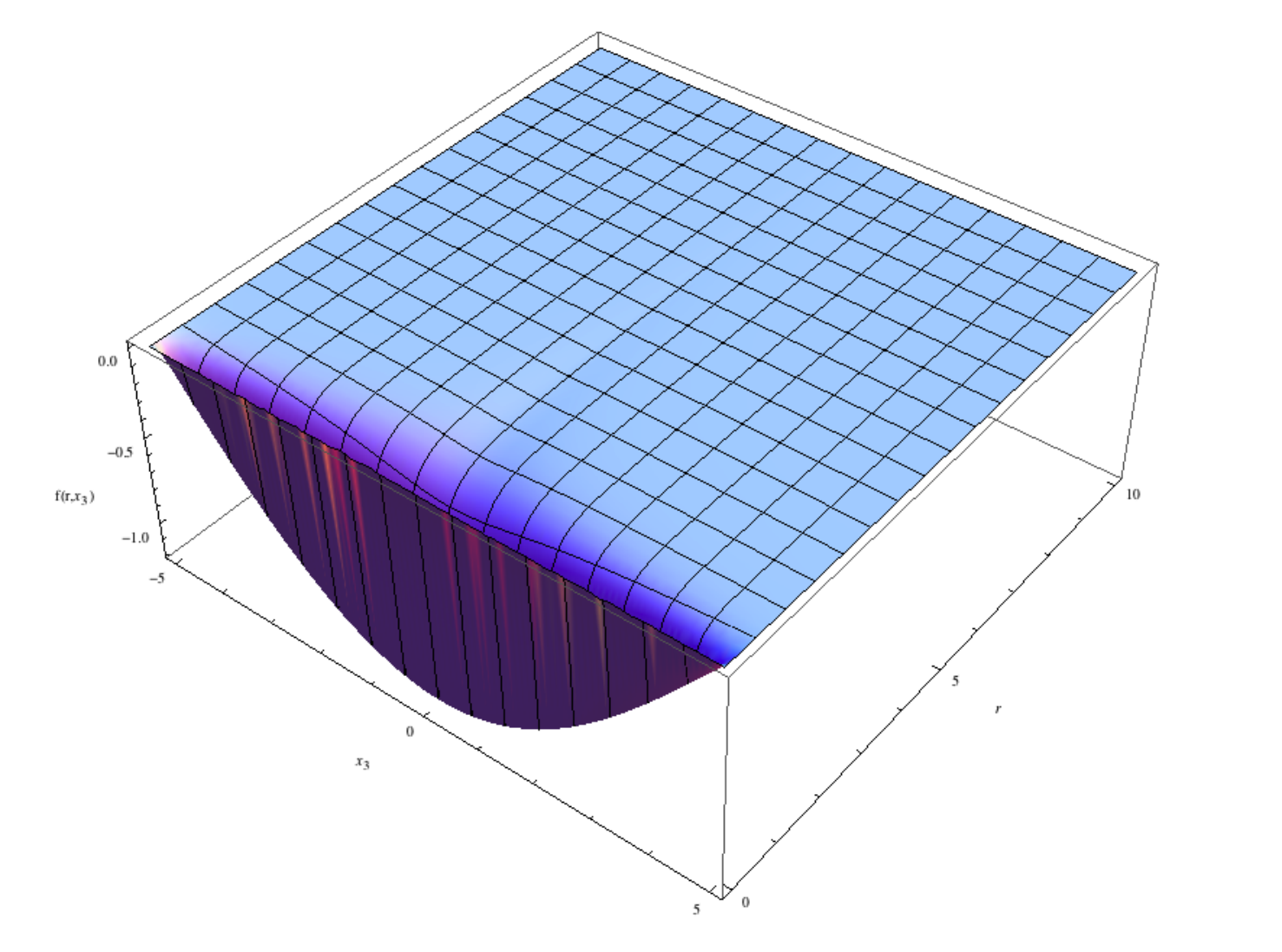
for large .
In particular we make dependent on an imaginary time . The derivative with respect to is given by the left-hand side of equation (5.10) multiplied by .
| (5.18) | |||||
After a sufficiently long time the field configuration approaches a solution of the right hand side equation. We solved this equation for a spatial region and . As a good initial function at time we use the first order solution (5.13) (with ) which we can trust for large . At the boundaries of the spatial regions, we impose Neumann boundary conditions for at and Dirichlet boundary conditions (given by the first order solution). The numerical solution of the equations was obtained using Mathematica and unlike the perturbative solution the numerical solution has the correct behavior both in the region and in the large region.
6 Discussion
Making coupling constants dependent on space time coordinates generically breaks all the supersymmetries of a supersymmetric field theory. Examples are Janus solutions [35] and the holographic topological insulator solutions constructed in [1]. Turning on a world volume gauge field allowed us to preserve four of the sixteen supersymmetries of the probe D7 brane. On the field theory side this corresponds to turning on localized counterterms as expected from the weak coupling analysis. A supersymmetric generalization of the topological insulator might be interesting in its own right from a theoretical perspective.
The BPS equations we have found are considerably simpler than the equations of motion, since they are first order instead of second order partial differential equations. Utilizing the scaling symmetry we have been able to generate exact smooth solutions. These solutions do however not have the boundary behavior which describes topological insulators. We have been unable so far to obtain closed form solutions corresponding to holographic topological insulators. Instead we had to resort to other methods such as perturbation theory and numerical methods. A closed form solution would be very useful as it is possible to study fluctuations about the solution and calculate correlation functions and transport quantities.
It is an interesting open problem to determine whether the difficulty of obtaining closed form solutions is a fundamental problem due to the small amount of preserved supersymmetry or simply due to the lack of ingenuity on the authors’ side55 5 Note that in the case of supersymmetric Janus solutions [24] the original form of the BPS equations looked too complicated to be solved. Only a sequence of clever variable changes made a solution possible..
Even with the numerical solutions it might be feasible to extract observable quantities, like transport quantities from the numerical solutions. We leave such questions for future work.
Acknowledgements
This work was in part supported by NSF grant PHY-07-57702. We are grateful to Carlos Hoyos, Kristan Jensen, Andreas Karch and Andy O’Bannon for useful conversations and correspondence. We are grateful to Brian Shieh for initial collaboration on this project. MG gratefully acknowledges the hospitality of the Newton Institute for Mathematical Sciences while this paper was finalized.
Appendix A Conventions
We will briefly review our conventions for the IIB supergravity and ten dimensional gamma matrices which follow [32]. The supersymmetry transformation parameters of type IIB supergravity can be written as a doublet
| (A.1) |
The flat space gamma matrices are matrices and the spinors are Majorana-Weyl spinors
| (A.2) |
The matrices in the -symmetry projectors are of the form
| (A.3) |
where and the Pauli matrices act on the doublet (A.1)
Appendix B Supersymmetry and counter-terms
In this appendix we review and adapt the results given in [30] for the field theory description of the topological insulator discussed in the body of the paper.
The theory is most conveniently formulated in terms in chiral multiplets, where only the supersymmetry is manifest. We consider chiral multiplets denotes with the field content.
| (B.1) |
where is a complex scalar, is a Majorana spinor and is an auxiliary field. In components the Lagrangian density is given by
| (B.2) |
where . The supersymmetry transformations are given by
| (B.3) |
Here is a Majorana spinor parameter. is the superpotential which parameterizes the self interactions of the chiral superfields. It was shown [30] that couplings in the superpotential which position dependent break all of the supersymmetries (B.3). Assuming that the superpotential depends on one coupling constant , the supersymmetry variation of the Lagrangian (B.2) is given by
| (B.4) |
is not a total derivative. Consequently, all supersymmetries are broken by the position dependent mass. Furthermore it was shown in [30] that some - but not all - supersymmmetries can be restored by adding a counter-term to the action of the form
| (B.5) |
The supersymmetry which is preserved is given by
| (B.6) |
For the theory discussed in section 3.1 the coupling is identified with the mass , the chiral superfields are identified with the superpotantial is given by
| (B.7) |
Appendix C D7 brane embedding
In this appendix we present the details of the D7 brane embedding for completeness. The background metric is given by
| (C.1) |
where
| (C.2) |
Note that we have introduced two different set of indices: and The corresponding coordinates and parametrize the field theory coordinates and the internal coordinates, respectively. The D7 brane world volume coordinates are identified with and In order to embed the D7 brane into we have to specify and as a function of the world volume coordinates. In this paper we restrict ourselves to
| (C.3) |
The induced metric on the world volume of the brane, with components is defined by
| (C.4) |
and takes the following form
| (C.5) |
where and The non-vanishing components of the field strength are, for
| (C.6) |
Note that and The pull back of the gamma matrices on the world volume (4.7) are given by
| (C.7) |
Appendix D Calculation of the -symmetry projector
In this appendix we will present the detailed calculation of and . We use the three projection conditions (4.11)-(4.13) as well as the properties of the world volume gauge field to bring the projector in a minimal form.
D.1 Calculation of
D.2 Calculation of
The contribution to which is linear in the field strength is given by
| (D.3) | |||||
where is the totally antisymmetric tensor in space normalized such that
We can use the formulae for the pull back of the gamma matrices (C.7) to determine
| (D.4) |
In addition we need the following relation involving the field strength
| (D.5) |
where the coordinates were defined in (3.2). There are three additional identities involving the field strength, which we need in the following
| (D.6) |
as well as
| (D.7) |
and
| (D.8) |
where we used the projection condition (4.12) to simplify the expressions above. Employing these identities together (D.3) can be expressed as follows
| (D.9) | |||||
This can be simplified by using (4.11),
| (D.10) | |||||
The dependence on the can be removed by employing (4.13) from which the following identities can be derived
| (D.11) |
Then the projector becomes
| (D.12) | |||||
D.3 Calculation of
The part of the projector which is quadratic in the field strength is given by
| (D.13) | |||||
Expressing the world volume gamma matrices in terms of flat space ones gives
| (D.14) |
and using the following relations which follow from the explicit ansatz for the gauge field (3.2)
| (D.15) |
we obtain
Using the projector (4.11) the expression can be simplified further to give
D.4 Final form of the projector
References
- [1] C. Hoyos-Badajoz, K. Jensen and A. Karch, “A Holographic Fractional Topological Insulator,” Phys. Rev. D 82 (2010) 086001 [arXiv:1007.3253 [hep-th]].
- [2] S. A. Hartnoll, “Lectures on holographic methods for condensed matter physics,” Class. Quant. Grav. 26, 224002 (2009) [arXiv:0903.3246 [hep-th]].
- [3] C. P. Herzog, “Lectures on Holographic Superfluidity and Superconductivity,” J. Phys. A A 42, 343001 (2009) [arXiv:0904.1975 [hep-th]].
- [4] J. McGreevy, “Holographic duality with a view toward many-body physics,” Adv. High Energy Phys. 2010, 723105 (2010) [arXiv:0909.0518 [hep-th]].
- [5] S. A. Hartnoll, C. P. Herzog and G. T. Horowitz, “Building a Holographic Superconductor,” Phys. Rev. Lett. 101, 031601 (2008) [arXiv:0803.3295 [hep-th]].
- [6] S. S. Gubser and S. S. Pufu, “The Gravity dual of a p-wave superconductor,” JHEP 0811, 033 (2008) [arXiv:0805.2960 [hep-th]].
- [7] G. T. Horowitz, “Introduction to Holographic Superconductors,” arXiv:1002.1722 [hep-th].
- [8] H. Liu, J. McGreevy and D. Vegh, “Non-Fermi liquids from holography,” Phys. Rev. D 83, 065029 (2011) [arXiv:0903.2477 [hep-th]].
- [9] M. Ammon, J. Erdmenger, M. Kaminski and P. Kerner, “Superconductivity from gauge/gravity duality with flavor,” Phys. Lett. B 680, 516 (2009) [arXiv:0810.2316 [hep-th]].
- [10] P. Basu, J. He, A. Mukherjee and H. -H. Shieh, “Superconductivity from D3/D7: Holographic Pion Superfluid,” JHEP 0911, 070 (2009) [arXiv:0810.3970 [hep-th]].
- [11] M. Ammon, J. Erdmenger, M. Kaminski and P. Kerner, “Flavor Superconductivity from Gauge/Gravity Duality,” JHEP 0910, 067 (2009) [arXiv:0903.1864 [hep-th]].
- [12] M. Ammon, J. Erdmenger, M. Kaminski and A. O’Bannon, “Fermionic Operator Mixing in Holographic p-wave Superfluids,” JHEP 1005, 053 (2010) [arXiv:1003.1134 [hep-th]].
- [13] J. L. Davis, P. Kraus and A. Shah, “Gravity Dual of a Quantum Hall Plateau Transition,” JHEP 0811, 020 (2008) [arXiv:0809.1876 [hep-th]].
- [14] C .L . Kane, ”An Insulator with a Twist” , Nature Physics 4, (2008) 348.
- [15] M. Z. Hasan and C. L. Kane, “Topological Insulators,” Rev. Mod. Phys. 82 (2010) 3045 [arXiv:1002.3895 [cond-mat.mes-hall]].
- [16] J. Moore, ”Topological insulators: The next generation”, Nature Phys. 5, (2009) 278.
- [17] X. L. Qi and S. C. Zhang, ”The quantum spin Hall effect and topological insulators” Physics Today 63, (2010) , 33-38.
- [18] X. -L. Qi, T. Hughes and S. -C. Zhang, “Topological Field Theory of Time-Reversal Invariant Insulators,” Phys. Rev. B 78 (2008) 195424 [arXiv:0802.3537 [cond-mat.mes-hall]].
- [19] R. Jackiw and C. Rebbi, “Solitons with Fermion Number 1/2,” Phys. Rev. D 13, 3398 (1976).
- [20] C. G. Callan, Jr. and J. A. Harvey, “Anomalies and Fermion Zero Modes on Strings and Domain Walls,” Nucl. Phys. B 250 (1985) 427.
- [21] J. Maciejko, X. -L. Qi, A. Karch and S. -C. Zhang, “Fractional topological insulators in three dimensions,” Phys. Rev. Lett. 105 (2010) 246809 [arXiv:1004.3628 [cond-mat.str-el]].
- [22] B. Swingle, M. Barkeshli, J. McGreevy and T. Senthil, “Correlated Topological Insulators and the Fractional Magnetoelectric Effect,” Phys. Rev. B 83 (2011) 195139 [arXiv:1005.1076 [cond-mat.str-el]].
- [23] J. Maciejko, X. -L. Qi, A. Karch and S. -C. Zhang, “Models of three-dimensional fractional topological insulators,” arXiv:1111.6816 [cond-mat.str-el].
- [24] E. D’Hoker, J. Estes and M. Gutperle, “Exact half-BPS Type IIB interface solutions. I. Local solution and supersymmetric Janus,” JHEP 0706 (2007) 021 [arXiv:0705.0022 [hep-th]].
- [25] E. D’Hoker, J. Estes and M. Gutperle, “Gravity duals of half-BPS Wilson loops,” JHEP 0706 (2007) 063 [arXiv:0705.1004 [hep-th]].
- [26] E. D’Hoker, J. Estes, M. Gutperle and D. Krym, “Exact Half-BPS Flux Solutions in M-theory. I: Local Solutions,” JHEP 0808 (2008) 028 [arXiv:0806.0605 [hep-th]].
- [27] M. Chiodaroli, M. Gutperle and D. Krym, “Half-BPS Solutions locally asymptotic to and interface conformal field theories,” JHEP 1002 (2010) 066 [arXiv:0910.0466 [hep-th]].
- [28] A. Karch, J. Maciejko and T. Takayanagi, “Holographic fractional topological insulators in 2+1 and 1+1 dimensions,” Phys. Rev. D 82 (2010) 126003 [arXiv:1009.2991 [hep-th]].
- [29] A. Karch and A. Katz, “Adding flavor to AdS/CFT,” Fortsch. Phys. 51 (2003) 759.
- [30] A. B. Clark, D. Z. Freedman, A. Karch and M. Schnabl, “The dual of Janus an interface CFT,” Phys. Rev. D 71 (2005) 066003 [arXiv:hep-th/0407073].
- [31] M. Kruczenski, D. Mateos, R. C. Myers and D. J. Winters, “Meson spectroscopy in AdS/CFT with flavour,” JHEP 0307 (2003) 049 [arXiv:hep-th/0304032].
- [32] E. Bergshoeff, R. Kallosh, T. Ortin and G. Papadopoulos, “kappa-symmetry, supersymmetry and intersecting branes,” Nucl. Phys. B 502 (1997) 149 [arXiv:hep-th/9705040].
- [33] A. Kehagias, “New type IIB vacua and their F-theory interpretation,” Phys. Lett. B 435 (1998) 337 [arXiv:hep-th/9805131].
- [34] M. Grana and J. Polchinski, “Supersymmetric three-form flux perturbations on AdS(5),” Phys. Rev. D 63, 026001 (2001) [arXiv:hep-th/0009211].
- [35] D. Bak, M. Gutperle and S. Hirano, “A Dilatonic deformation of AdS(5) and its field theory dual,” JHEP 0305 (2003) 072 [hep-th/0304129].