eurm10 \checkfontmsam10
Resonant behaviour of an oscillating wave energy converter in a channel
Abstract
A mathematical model is developed to study the behaviour of an oscillating wave energy converter in a channel. During recent laboratory tests in a wave tank, peaks in the hydrodynamic actions on the converter occurred at certain frequencies of the incident waves. This resonant mechanism is known to be generated by the transverse sloshing modes of the channel. Here the influence of the channel sloshing modes on the performance of the device is further investigated. Within the framework of a linear inviscid potential-flow theory, application of the Green theorem yields a hypersingular integral equation for the velocity potential in the fluid domain. The solution is found in terms of a fast-converging series of Chebyshev polynomials of the second kind. The physical behaviour of the system is then analysed, showing sensitivity of the resonant sloshing modes to the geometry of the device, that concurs in increasing the maximum efficiency. Analytical results are validated with available numerical and experimental data.
keywords
Authors should not enter keywords on the manuscript, as these must be chosen by the author during the online submission process and will then be added during the typesetting process (see http://journals.cambridge.org/data/relatedlink/jfm-keywords.pdf for the full list)2Centre de Mathématiques et de Leurs Applications (CMLA), Ecole Normale Supérieure de Cachan, 94235 Cachan, France
1 Introduction
Renewed interest in wave power extraction has arisen in the recent years, following the need for clean energy resources alternative to fossil fuels. As a consequence, a lot of work has been done recently to discover effective design layouts for wave energy converters (see McCormick, 2007; Cruz, 2008, for an extensive review of wave energy conversion techniques). The work of Folley et al. (2005) and Whittaker et al. (2007) on a number of different devices showed that an effective solution to harness energy from water waves is represented by oscillating wave energy converters. Their simplest form is that of a buoyant flap hinged at the bottom of the ocean and has been named Oscillating Wave Surge Converter (OWSC). Under the action of incoming incident waves, the flap is forced to a pitching motion about the hinge, that is eventually converted into energy with the use of a generator. The converter is naturally placed in shallow waters, where the pitching of the flap combines well with the amplified horizontal motion (surge) of the fluid particles (hence the name OWSC). During the wave tank tests of Whittaker et al. (2007), Henry (2008) and van’t Hoff (2009), peaks in the hydrodynamic actions on the converter occurred at certain frequencies of the incident waves. This resonant phenomenon is known to be due to the excitation of the transverse sloshing modes of the channel (Shemer et al., 1987). However, there is still uncertainty on how the resonant transverse waves interact with the device and affect its efficiency (van’t Hoff, 2009). Here we address this unresolved issue by developing a three-dimensional mathematical model of an oscillating wave energy converter, namely the OWSC, inside a channel. Although much analytical modelling has been done for a large number of wave energy converters (WECs) (see Falnes, 2002; Mei et al., 2005; McCormick, 2007, for a collection of theories on WECs), few analytical studies are available in the literature concerning OWSCs.
Indeed, the hydrodynamics of flaps has been widely studied in the past due to their usage as wavemakers (see Dean & Dalrymple, 1991, for a compendium of wavemaker theories), with Milgram (1970) being among the first to suggest the employment of a moving paddle not only as a wave generator, but also as a wave energy absorber. Later on, the hydrodynamic characteristics of flat plates have been studied by Parsons & Martin (1992); Parsons & Martin (1994); Parsons & Martin (1995) and more recently by Evans & Porter (1996) for both submerged and surface-piercing plates. In particular, the work of Parsons & Martin (1992) is a seminal example of the application of hypersingular integral equations to problems in water waves. Nevertheless, all these analytical studies deal with two-dimensional (2D) geometries. Hence they are inadequate to describe the complex three-dimensional (3D) behaviour of the wave field around the flap noticed in the experimental analysis of the OWSC. A non-linear 3D analytical model has been developed by Mei et al. (1994) and Sammarco et al. (1997) for the flap gates of the barriers designed to protect Venice from flooding. Mei et al. (1994) and Sammarco et al. (1997) showed that trapped modes exist near a barrier of oscillating flaps in a channel. Since the narrowly spaced flaps span the whole channel width, this system is closed and can resonate only subharmonically (i.e. non-linearly). The work of Sammarco et al. (1997) aims at reducing the resonant effects that could lead to undesired large oscillations of the flaps, thus undermining the effectiveness of the barrier.
Going back to wave energy, a wise design of the OWSC should exploit the beneficial effect of resonance in enhancing the amplitude of oscillation of the flap, thus allowing to capture more wave power. For bodies of various geometries in a channel, Eatock Taylor & Hung (1985), Yeung & Sphaier (1989), Linton & Evans (1992) and Chen (1994) already showed that linear resonance mechanisms influence the radiation and diffraction properties significantly. This influence manifests itself by the presence of peaks in the hydrodynamic characteristics of the system, at periods corresponding to the resonance of symmetric transverse standing waves within the channel lateral walls. As already mentioned, similar dynamics has been shown to occur also during wave tank tests of the OWSC, rising the following questions: (i) how linear resonance of transverse waves is triggered for a typical OWSC configuration in a channel, (ii) how do the transverse sloshing modes interact with the OWSC and modify its performance, and (iii) to what extent the results obtained in an experimental wave tank can be applied to predict the behaviour of the device in the open ocean.
A mathematical model of the OWSC in a channel is developed in the following sections to address the above points. The fluid is assumed to be inviscid and incompressible, the flow irrotational, the perturbation time harmonic. In §2 the governing equations are scaled and linearised according to first-order potential flow theory. The hydrodynamic problem is then decomposed into a radiation and a diffraction problem, which are solved separately using the hypothesis of thin plate and eventually summed up to obtain the total potential. The solution is achieved with the integration of a hypersingular problem, resulting from the application of the Green theorem to the physical domain. In §3 the hydrodynamic characteristics of the system, such as the excitation torque, added inertia torque and radiation damping are fully investigated and the efficiency of the OWSC is assessed. Analytical results agree well with available numerical and experimental data. It is shown that all the above quantities are characterised by the occurrence of spikes at the cut-off frequencies of the transverse sloshing modes. The latter are excited in the channel by the diffraction of the incident wave field at the edges of the flap and influence the performance of the OWSC. Finally, a parametric analysis reveals how the transverse modes can increase the efficiency of the device, depending on the geometry of the system.
2 Analytical model
2.1 Governing equations
Referring to figure 1(), consider an OWSC in water of depth , where the prime indicates a physical dimensional quantity.

For the sake of generality, we shall represent the converter by a rectangular flap of width and thickness , hinged along a straight axis upon a rigid platform, at a distance from the bottom of the ocean (see figure 1). The device is located in the middle of a straight channel, whose impermeable walls are placed at a mutual distance and extend to infinity to either side (see figure 1). Incident waves are coming from the right with wave crests parallel to the OWSC and set the flap into an oscillating motion. This is eventually converted into useful energy by means of a generator linked to the device. Note that, due to the mirroring effect of the side walls, the layout of figure 1() can also be employed to model the behaviour of an infinite array of identical OWSCs in the open ocean, subject to beam seas. The converters in this array have spatial period and oscillate at unison. Returning to the channel layout, let us now define a plane reference system of coordinates . Let lie on the centre line of the channel, along the axis of the OWSC at rest position and rise up from the undisturbed water level , positive upwards. The flap is able to oscillate on the vertical plane about the horizontal axis at , thus representing a system with one degree of freedom, i.e. pitch. Its time-dependent amplitude of rotation is defined positive if counter-clockwise; denotes time. We also assume that the bottom foundation does not oppose the flap movement (Sammarco, 1996, ideal foundation, see) and that the hinge is frictionless. As in many gravity-wave problems (Mei et al., 2005, see for example) the fluid is deemed to be inviscid and incompressible and the flow irrotational. Hence there exists a potential for the velocity field , where is the nabla operator. Subscripts with commas denote differentiation with respect to the relevant variable. The complete set of nonlinear equations governing the system is detailed in Appendix A. Since the resonance of the channel sloshing modes is a linear phenomenon (Shemer et al., 1987), here we shall consider a linearised theory. The first-order analysis presented in this paper constitutes the basis for further investigation of higher-order phenomena occurring in the system (see §3). Now let denote the amplitude scale of the wave field and the acceleration due to gravity. Then introduce the following non-dimensional variables
| (1) |
where is the physical scale of the angular rotation, and constants
| (2) |
The linear governing equations are derived in the limit of small-amplitude oscillations of the flap, i.e. , by considering the terms in the fully nonlinear system (49)–(57) scaled according to (1). The potential is governed by the Laplace equation
| (3) |
where is the fluid domain. On the free-surface, the kinematic-dynamic boundary condition reads
| (4) |
The no-flux conditions on the solid boundaries require
| (5) |
on the channel lateral walls and
| (6) |
on the bottom. Allowing only tangential motion along the lateral surfaces of the OWSC yields
| (7) |
where denotes the Heaviside step function. Finally the linearised equation of motion of the flap reads
| (8) |
where is the elastic moment of inertia due to net buoyancy, and are respectively the first and second moment of inertia of the flap and is the first-order torque exerted by the generator on the flap, all in non-dimensional variables; is water density. Without loss of generality, we shall assume to depend on time via and to be partly inertial, partly elastic and partly damping (see Mei et al., 2005, for a similar example)
| (9) |
In the latter expression and are respectively the inertial and elastic characteristic of the generator, while is the energy extraction rate. Now note that the physical scale of the OWSC width is (Henry, 2008), so that . Hence the thickness of the OWSC can be neglected if compared to the reference length scale and the hypothesis of thin obstacle (Linton & McIver, 2001) can be applied to evaluate the potential . As a consequence, in the boundary condition on the lateral surfaces (7) and in the right-hand side of the equation of motion (8).
2.2 Solution of the radiation and scattering problems
In this section solution is found to the Laplace equation (3) with linearised boundary conditions (4) on the free-surface, (5) on the channel walls, (6) on the bottom and (7) on the flap lateral surfaces. Once having solved this system, expression (8) will be employed to determine the motion of the flap. Assume that the flap undergoes simple harmonic oscillations of frequency about its rest position, so that
| (10) |
where Re is the real part and the complex amplitude of rotation. Position (10) allows to separate the time factor in the time-dependent variables, so that the velocity potential can be rewritten as
| (11) |
where the symbol Re is omitted for the sake of brevity. Due to the linearity of the problem, the spatial potential is analysed by resorting to the classical decomposition (Linton & McIver, 2001; Mei et al., 2005, see for example)
| (12) |
In the latter, is the solution of the radiation problem, in which the flap is set to oscillate without incoming incident waves, and is the solution of the scattering problem, where the flap is held fixed in incoming waves. In turn, the scattering potential can be decomposed into
| (13) |
where
| (14) |
is the potential of the incident wave and the potential of the diffracted waves (Linton & McIver, 2001; Mei et al., 2005, see). In (14) and are respectively the non-dimensional incident wave amplitude and wavenumber, the latter depending on the wave frequency according to the dispersion relation . In the following, the radiation and scattering problems will be investigated and their results summed up to obtain the total wave field.
The boundary-value problems for the radiation potential and the diffraction potential can be determined by employing the factorizations (10)–(11) and the decompositions (12)–(13) into the governing equations (3)–(7). As a consequence, and must satisfy the Laplace equation
| (15) |
where the shorthand notation denotes either potential, the kinematic-dynamic boundary condition on the free-surface
| (16) |
the no-flux condition on the bottom
| (17) |
and on the channel walls
| (18) |
and the kinematic conditions on the lateral surfaces of the flap
| (19) |
Finally, must be outgoing at large . Separation of variables
| (20) |
yields the well-known vertical eigenmodes (Mei et al., 2005, see for example)
| (21) |
which satisfy the orthogonality relation
| (22) |
being the Kronecker delta, . In (21)
| (23) |
are the solutions of the dispersion relationships
| (24) |
respectively. Hence an equivalent form of (21) for is , i.e. an oscillating function of . By making use of (20) and (21), the Laplace equation (15) becomes
| (25) |
governing the plane radiation and diffraction potentials in the 2D fluid domain (see figure 1), where will be omitted from now on for brevity. Note that (25) is an ordinary Helmholtz equation when , for which , and a modified Helmholtz equation when , for which . With the same steps as above, the no-flux condition on the channel walls (18) gives
| (26) |
Now consider the kinematic conditions on the flap (19). Using the factorization (20), multiplying both sides by , integrating along the vertical line from to and using the orthogonality relation (22) yields
| (27) |
In the latter expression
| (28) |
is the complex angular velocity of the flap, while
| (29) |
and
| (30) |
are real constants depending on the modal order . Finally must be outgoing disturbances along the channel. In summary, the 2D -th mode potentials must solve the Helmholtz equation (25) with the boundary conditions (26)–(27) and be outgoing. Here we shall solve this boundary-value problem by employing an integral-equation method based on the application of Green’s theorem with an appropriate channel Green function. In the literature Achenbach & Li (1986) and Martin & Rizzo (1989) already used a similar procedure to solve plane sound-wave problems, while Parsons & Martin (1992); Parsons & Martin (1994); Parsons & Martin (1995) applied this method to the scattering and trapping of surface waves by plates. Later, Martin & Farina (1997) used the integral-equation approach to solve the radiation problem for a heaving submerged horizontal disc, but without bounding walls and in water of infinite depth. In this paper, the boundary-value problem (25)–(27) is solved in Appendix B by applying an integral-equation technique based on the decomposition of the Green function into a singular part and an analytical remainder. Such a procedure is inspired by Chen (1994)’s analysis of the tank Green function for numerical models. The integral-equation technique allows to solve the plane boundary-value problems for and ultimately to express the potentials (20) in an appealing fast-converging semi-analytical form (see Appendix B for details). The radiation potential is given by
| (31) |
where is the Hankel function of the first kind and first order and the are the Chebyshev polynomials of the second kind and order . Finally, the are the complex solutions of the linear system of equations (96) which ensures that the boundary condition on the plate (27) is satisfied. This system is solved numerically with a collocation scheme (see again Appendix B), therefore the solution is partly numerical. Note that the radiation potential (31) is an odd function of , as suggested by the antisymmetric pitching motion of the flap. Physically, (31) represents the sum of outgoing waves within the waveguides imposed by the lateral walls and is similar in form to the solutions of other problems of water waves propagating past sharp obstacles (see for example Evans & Porter, 1997; Lovas et al., 2010, who also employ Chebyshev polynomials). The inner series in (31) represents a sum of disturbances radiated by sources arranged periodically along the axis and converges as for large . Numerically, summation from up to ensures convergence of the series with relative error close to resonance and elsewhere. The central series in (31) is truncated at and its coefficients are calculated numerically as described in Appendix B. Numerical investigation showed that is sufficient to ensure convergence with virtually no relative error. The outer series in (31) over the vertical eigenmodes was found to converge quickly already for with a relative error . Hence the method of solution adopted here, based on the appropriate decomposition of the Green function (63)–(65), proves to be reliable and computationally efficient. Turning to the scattering problem, the diffraction potential is given by
| (32) |
In the latter expression the are the complex solutions of the linear system of equations (96) for , which ensures that the no-flux condition on the flap (19) is satisfied. Thanks to linearity, the total potential is obtained by simply summing up the solutions (31) and (32) of the radiation and diffraction problem, respectively, to the incident wave potential (14). The equation of motion of the flap can now be solved.
2.3 Flap motion
2.3.1 Hydrodynamic parameters
Consider the law of motion of the flap (8). By using the factorizations (10) and (11) for and respectively, applying the decomposition , employing the solutions (31) and (32) for and respectively and expressing with (9), (8) yields
| (33) |
In the latter expression is the unknown complex amplitude of rotation of the flap, while
| (34) |
is the added torque due to inertia and
| (35) |
is the radiation damping, both depending on the solutions to the linear system (96) for the radiation problem. Finally
| (36) |
is the complex excitation torque, corresponding to the action on the plate as if it was held fixed in incoming waves.
2.3.2 Extracted power and capture factor
Expression (33) formally describes a simple harmonic oscillator in the frequency domain; hence the average extracted power from the OWSC over a period is
| (37) |
where again and is the solution of (33). Returning to physical variables via (1), the power take-off expressed in Watts is then
| (38) |
The rate of power take-off (37) can be maximized according to the optimizing criteria
In the latter, condition ( ( 39 a , b ) ) corresponds to the tuning between the incident wave frequency and the natural pitching frequency of the flap, while ( ( 39 a , b ) ) requires the equality of the rate of power take-off to the radiation damping (35). A quick numerical assessment of the tuning condition ( ( 39 a , b ) ) for a typical OWSC configuration (see §3.1) reveals that the natural pitching period is larger than the ordinary wave periods on site, about (Henry, 2008). Hence the tuning condition ( ( 39 a , b ) ) is not achieved in normal operating circumstances. Away from body resonance, the extracted power (37) can still be optimized by adjusting the damping rate such as , which yields
| (40) |
as the optimum damping rate (Falnes, 2002, see). Then the optimum power is obtained by substituting in (37). Now, the rate of extracted power and the optimum power are functions of the wave climate, so that the amount of energy extracted from a given floating body strongly depends on the sea state. Therefore both the rate of power take-off and the optimum power are not reliable indicators of the efficiency of the system (Cruz, 2008). A more rational efficiency assessment is done by considering the capture factor, defined as the ratio between the optimum power extracted per unit flap width and the power of the incident wave field per unit crest length, i.e.
| (41) |
where and
| (42) |
are respectively the amplitude and the group velocity of the incident waves in physical variables. In the following, all the parameters describing the performance of the OWSC will be assessed in physical variables.
In the next sections, the analytical theory will be validated against numerical and experimental models. Discussion will follow on the physical behaviour of the system and further analysis will investigate the dependence of the system on its main parameters, such as the frequency of the incident waves and the width of the flap. Resonance will be shown to occur at special frequencies, namely the cut-off frequencies of sloshing waves in open channels. The response curves of the system dynamic characteristics show that the OWSC performance is largest under resonance conditions.
3 Discussion
3.1 Numerical and experimental comparison
In order to validate the theory, comparison is made with the numerical results of van’t Hoff (2009). In the analytical model, the width of the flap is , while the width of the channel is , giving a blockage ratio . The depth of the channel is and the distance between the bottom and the hinge is . The amplitude of the incident wave is , which gives . This justifies the assumption of linear theory for this case. The numerical data have been obtained with the software package WAMIT (WAMIT Inc., 2008) for the linear analysis of the interaction of surface waves with offshore structures. The geometry of the flap used in the numerical simulations is that of an wide rectangular box standing on a triangular prism pointing downwards (see van’t Hoff, 2009, for specifications). The flap in turn is hinged on a high rectangular platform lying on the bottom of a deep ocean. In the numerical calculations of van’t Hoff (2009) the device is placed in open water, so that the model does not simulate the effect of the lateral walls. Figures 2() and 2(), respectively, show the values of the added inertia torque and the absolute value of the excitation torque in physical variables versus the wave period , for both the analytical and the numerical model.

While in the analytical model the flap has zero thickness, in the numerical model the simulations have been carried on with different non-zero values of the total thickness (see again figure 2,). The agreement between both models is satisfactory. However for the added inertia torque (figure 2), the analytical values are slightly larger than the numerical ones. This is likely due to the differences in the shape of the flap, a perfect rectangular box in the analytical model and a rectangular box sitting on a triangular base in the numerical model. Also, note that the analytical values are larger than the numerical ones next to the peaks of either the added inertia torque ( in figure 2) and the excitation torque ( in figure 2). This is a consequence of the bounding effect of the lateral walls, absent in the numerical model of van’t Hoff (2009), that will be discussed in depth in §3.2. Finally, the numerical results in figure 2(,) clearly show that the hydrodynamic coefficients do not vary noticeably while varying the flap thickness. The initial assumption of neglecting the thickness of the flap to calculate the hydrodynamic actions, namely the thin-plate approximation, is then validated. The theoretical results of §2 are further validated by comparison with the data of Henry (2008). These have been obtained during an experimental campaign at Queen’s University Belfast on a scale model of the OysterTM wave energy converter developed by Aquamarine Power Ltd 11 1 www.aquamarinepower.com (Folley et al., 2007; Whittaker et al., 2007; Henry et al., 2010, see) having similar dimensions to those already specified for the theoretical models. In figure 3 the behaviour of the excitation torque with the incident wave period is reported for both the equivalent analytical box-shaped flap and the experimental model of the OysterTM WEC.

Very good agreement is found between the two sets of data: the theoretical model described in §2 is also capable to simulate the behaviour of a real - and more complex - OWSC.
3.2 Resonance
After having shown a good agreement between the analytical and the numerical/exper- imental data, we shall investigate in more depth the 3D dynamics of the flap in the channel and the influence of the channel lateral walls in enhancing the efficiency of the converter. First, let us consider the diffraction problem and analyse the modifications induced by the 3D wave field in the 3D channel model of §2 with respect to a simplified reference model, in which , i.e. the flap spans the entire width of the channel. Here the behaviour of the fluid is clearly two dimensional, so that this layout will be referred to as the 2D channel. As already demonstrated in the literature (Linton & McIver, 2001; Falnes, 2002), the excitation torque acting on the flap in the 2D channel is, in physical variables,
| (43) |
In figure 4 the excitation torque is plotted against the wave period in physical variables, for either the 3D-channel model of §2 and the 2D-channel reference model.

While the 2D excitation torque regularly increases with the period up to the asymptotic long-wave value
| (44) |
the 3D torque reaches its maximum value at a finite period . Then it decreases while moving towards longer periods, with a secondary spike at . Hence an immediately noticeable effect of the 3D dynamics is the lowering of the peak period to finite values. Though the two curves of figure 4 have a very different aspect, they show the interesting property that (see again figure 4). Hence to further study the 3D effects on the system, it is convenient to consider the non-dimensional ratio
| (45) |
between the excitation torque in the 3D channel and the maximum excitation torque in the 2D channel. In figure 5() is plotted versus the non-dimensional wavelength of the incident wave, for the same geometry as above.

The graph of figure 5() exhibits the typical spiky behaviour already noticed by Achenbach & Li (1986) when studying the reflection coefficients for normal incidence of sound waves on an array of screens. Similar spikes have also been found by Eatock Taylor & Hung (1985), Yeung & Sphaier (1989), Linton & Evans (1992) and Chen (1994) in the analysis of the hydrodynamic coefficients of bodies of various shapes in a channel. Note that in figure 5() the spikes, either in the form of local maxima or changes in slope, occur at special values of , i.e. The latter correspond to the well-known values of the cut-off wavelengths of the symmetric sloshing modes in a channel (Shemer et al., 1987; Mei et al., 2005, see for example)
| (46) |
The sloshing modes are transverse standing waves whose crests are parallel to the axis of the channel, oscillating back and forth between the two bounding lateral walls. The physical behaviour of the sloshing waves is strongly dependent on the width of the channel and on the wavelength of the incident wave. As shown by Mei et al. (2005), if , then the -th sloshing component propagates along the channel, carrying the associated wave energy towards infinity. On the other hand, if , the amplitude of the -th sloshing mode decays exponentially while moving along the channel. In our case, this means that the energy associated to these modes is trapped near the OWSC and available for extraction. A further insight on this fundamental influence of the sloshing modes can be achieved by considering the ratio between the -th sloshing mode group velocity (Mei et al., 2005, see) and the group velocity of the incoming waves (42), i.e.
| (47) |
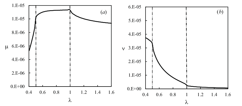
Recall that the group velocity is the speed of energy transport. As soon as , and the energy of the -th sloshing mode is no longer propagating along the channel: the sloshing mode is trapped near the flap. Figure 5() shows the behaviour of the group velocity ratio (47) for the first three sloshing modes versus the wavelength of the incident wave. Let us first consider the group velocity ratio for the mode (dotted line). When , the group velocity ratio quickly decays to zero, so that the third sloshing mode is now trapped near the flap. The trapping of the energy associated to this mode determines a sudden increase of the excitation torque acting on the flap, which results in having a spike at , as shown in figure 5(). By further increasing , the group velocity ratio of the second sloshing mode quickly decays too, being for (dashed line of figure 5). Due to the trapping of the second sloshing mode, the excitation torque acting on the flap further increases, leading to the peak of occurring exactly at the cut-off frequency of the second sloshing mode, (see figure 5). Additionally increasing makes the incoming waves so long that they pass through the flap almost as a uniform swelling. As a consequence, the net pressure acting on the flap diminishes, leading to a decrease of the excitation torque which also reflects on (see again figure 5). Nevertheless, as soon as , (see the solid line in figure 5) and the first sloshing mode is also trapped near the flap. This results in having a ultimate spike at , as shown in figure 5(). The physical picture is now clear. The incoming plane waves, initially 2D, impact the flap in the middle of the channel. Differently from the 2D channel, in which the incident waves are totally reflected back to the source, in the 3D channel the waves are also transmitted beyond the flap, due to the lateral gaps between the body and the channel walls. Diffraction at the edges of the flap modifies the behaviour of the wave field and dominates the shape of the hydrodynamic coefficient curves, making them different from the 2D scenario (see figure 4). As a consequence of this enriched dynamics, transverse sloshing modes, a feature of the channel, are ultimately excited. Hence the initial 2D motion shatters into a series of symmetric 3D sloshing waves, resonating each at its own cut-off frequency. When a sloshing mode resonates, the relevant energy is trapped near the flap, resulting in an increase of the excitation torque. Similar conclusions can be drawn also for the radiation problem, where the waves are generated by the pitching motion of the plate. Figure 6() shows the plots of the added inertia torque (34) and the radiation damping (35) versus the wavelength of the generated waves in non-dimensional variables. Note that spikes occur here at the same resonant wavelengths as those of (45) for the scattering problem (see again figure 5). This correspondence is due to the relationship between the radiation and scattering problems
shown in Appendix C, for which the excitation torque acting on the fixed flap in incoming waves is associated to the radiation potential of the pitching motion of the body. We now investigate the OWSC performance.
3.3 Wave power extraction
After having analysed the radiation and scattering problems separately, we now turn to study the performance of the OWSC in terms of wave power extraction. First, let us consider the flap pitching amplitude , solution of (33). For easiness of representation, but without loss of generality, in expression (33) we take the generator inertial and linear terms and make use of the optimizing criterion (40) for the rate of power take-off, such that . Finally, we use the values of the moment of inertia and buoyancy factor for a typical configuration of the OysterTM wave power device (private communication with Aquamarine Power Ltd). In figure 7() the absolute value of the flap pitching amplitude is plotted versus the period of the incident wave in physical variables.

Note that the amplitude of oscillation of the flap increases smoothly while moving to longer waves, not showing the characteristic spiky behaviour of the hydrodynamic coefficients. Since is related to the displacement in the direction via the pitching movement of the flap, it seems unaffected by the sloshing modes resonating in the orthogonal direction. Let us now consider the capture factor , defined by (41) as a measure of the OWSC efficiency in catching the energy available in incident waves. In figure 7() the capture factor is plotted against the incident wave period. Comparison between figures 4 and 7() reveals that both the excitation torque and the capture factor have a peak at , which corresponds to the resonant period of the second sloshing mode. Hence the capture factor is dominated by the excitation torque, which is the power generating action. Overall, figure 7() reveals that the average capture factor of the 3D-channel model is larger than the maximum theoretical value of the 2D-channel model (Mei et al., 2005, see for example). This shows again that the 3D dynamics described in §3.2 altogether increases the efficiency of the device with respect to the 2D layout. Finally, the maximum capture factor at resonance is , indicating that the interference between the transverse sloshing modes occurring in the 3D channel can further enhance the OWSC performance. Resonance of the sloshing modes is therefore beneficial for wave energy extraction. Despite the fact that the dynamics of the OWSC in the channel is affected by the bounding effect of the lateral walls, the general behaviour of the device in the open ocean can also be inferred. There the dominant physical mechanism is still the transmission of the incident waves beyond the flap, but no sloshing modes are present. Hence the OWSC is expected to perform in the open ocean similarly as it does in the 3D channel, exception made for the narrow bandwidths close to the resonant frequencies of the sloshing modes. However, to simulate properly the behaviour of a single device in the open ocean a different mathematical model is needed, in which the waves are allowed to propagate in all directions. In summary, care should be taken when using experimental results obtained in wave tank testing as a benchmark for predicting real on-site behaviour. In the following we shall investigate the influence of the system main parameter, namely the width ratio , on the performance of the OWSC.
3.4 Parametric analysis and further research directions
The response of the capture factor (41) to variations of the flap width is shown in figure 8. Here the plots of against the wave period are shown for different widths of the OWSC, i.e. (corresponding to ), () and (), for fixed width of the channel, .
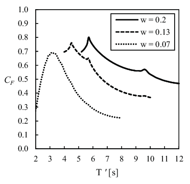
Note that for all widths the capture factor is largest in short periods, thus matching the experimental observations of Whittaker et al. (2007). Indeed at larger periods (not shown here), tuning of the incoming wave frequency with the natural pitching frequency of the flaps ( ( 39 a , b ) ) can occur, thus yielding additional peaks in the capture factor curves. Unfortunately, this event is unlikely to occur in normal operating conditions of the device (Henry et al., 2010) and won’t be investigated here. Further examination of figure 8 also reveals that the wider the flap the larger the capture factor, for a given width of the channel. This fundamental result, already noticed experimentally by Henry (2008) and Henry et al. (2010), reveals a selective behaviour of the sloshing modes with respect to the width of the flap, for which the most powerful resonance occurs with the largest flaps. Now, to what extent can we increase the flap width to exploit this mechanism, in a channel of fixed width? Of course, growth in the structural loads on the device is a heavy limit on the enlargement of the flap (Henry, 2008). Hence we consider the alternative way of decreasing the width of the channel, while holding fixed. By decreasing so that , the width of the channel becomes comparable to the width of the flap. Hence the 3D effects become less noticeable, the geometry approaching that of a 2D device. Figure 9 shows a preliminary analysis of the torque with the incident wave period for .

Here 3D effects are largely inhibited by the body, so that the device shows a “quasi-2D” behaviour (Yeung & Sphaier, 1989). As a consequence, when the selective behaviour of the sloshing modes is expected to have a weaker impact on the performance of the OWSC, whose maximum efficiency will decrease closer to the theoretical 2D values. This suggests that an optimal layout maximising the resonant actions on the device must lie in between the two extremes (open ocean) and (2D channel). A supplementary investigation of the response of the system to variations of the channel width is then needed. This analysis is currently ongoing and will be disclosed in the near future.
Finally, recall that resonance of sloshing modes is a linear mechanism. Nevertheless, resonant mechanisms can also excite the second-order transverse modes (Shemer et al., 1987, cross waves, see). A preliminary numerical analysis with a weakly nonlinear Boussinesq model showed nonlinear amplification of the dynamic pressure on the flap to occur near the cross-wave resonant frequencies (Schmitt et al., 2012, see). A nonlinear mathematical model based on the governing equations of Appendix A and on the linear results obtained here is to be developed to investigate whether the nonlinear interactions can further increase the performance of the device.
4 Conclusion
A mathematical 3D model of an oscillating wave energy converter (i.e. the OWSC) in a channel is developed to investigate the influence of the channel sloshing modes on the performance of the system, in a layout common to many experimental studies (Folley et al., 2005; Whittaker et al., 2007; Henry et al., 2010, see). The linearised theory, based on the solution of a hypersingular problem in the fluid domain, is satisfactorily validated by comparison with numerical and experimental models (van’t Hoff, 2009; Henry, 2008, see respectively). When the flap is set to oscillations by incident waves, the incoming 2D wave field is modified by the diffraction occurring at the edges of the flap and by the waves radiating from the device. Then a complex 3D wave field develops in the channel, increasing the average efficiency of the OWSC with respect to that of a 2D pitching flap. In addition, this 3D dynamics leads to the excitation of transverse sloshing waves which resonate each at its own cut-off frequency. Transverse modes trapped near the flap are responsible for the spiky behaviour of the hydrodynamic characteristics of the system and further increase the efficiency of the device near resonance. Finally, parametric analysis reveals a selective behaviour of the sloshing modes, whose resonant capacity depends on the width of the device. In response to the three issues we anticipated in the introductory section, we conclude that (i) resonance of the channel sloshing modes is a linear mechanism and occurs for every width of the flap; (ii) the sloshing modes show a selective behaviour with respect to the width of the flap, that concurs in increasing the performance of the device near resonance; (iii) care should be taken when employing the results obtained in an experimental wave tank to predict the behaviour of the device in the open ocean, especially near resonant frequencies.
This work was funded by Science Foundation Ireland (SFI) under the research project “High-end computational modelling for wave energy systems”. Numerical simulations of van’t Hoff (2009) and experimental data provided by Henry (2008) in agreement with Aquamarine Power Ltd have been very useful for the validation of the model. Fruitful discussions with Prof. P. Sammarco, Dr K. Doherty and Dr S. Bourdier are kindly acknowledged. The Authors wish to thank the wave research group at Queen’s University Belfast for having let them partake in the June 2011 experimental campaign.
Appendix A Nonlinear governing equations
Consider the geometry of figure 1 representing the OWSC in the channel as described in §2. During the motion, the position of each side of the converter (made up by the bottom foundation and the flap) is at , where
| (48) |
In the latter, the () superscript denotes the right (left) side of the OWSC and is the free-surface elevation along the wetted line of the flap on the right (left) lateral surface (see figure 1). Clearly, in (48) the upper equivalence holds for all points on the fixed bottom foundation, while the lower one is valid on the lateral surfaces of the moving flap. As in many gravity-wave problems (Mei et al., 2005, see for example) the fluid is deemed to be inviscid and incompressible and the flow irrotational. Hence there exists a potential for the velocity field such that
| (49) |
where is the fluid domain. To set up a boundary-value problem governing the behaviour of the fluid in , the Laplace equation (49) must be supplied with appropriate boundary conditions. On the free-surface, the kinematic-dynamic boundary condition reads
| (50) |
where is the acceleration due to gravity. In (50) the free-surface elevation is obtained via the Bernoulli equation
| (51) |
where is the water density and the fluid pressure. By evaluating (51) at and considering only the excess pressure over the atmospheric value, the free-surface elevation is
| (52) |
Boundary conditions must also be applied at the solid frontiers delimiting the domain. We require absence of normal flux through the channel walls
| (53) |
through the moving sides of the OWSC parallel to the -axis
| (54) |
and through the impermeable bottom of the channel
| (55) |
Finally, a kinematic boundary condition allowing only tangential motion along the lateral surfaces of the OWSC is to be applied. Following the reasoning of Sammarco (1996) for the mobile gates of the Venice storm barriers, we require , which yields
| (56) |
where (48) has been employed. In (56) usage of the Heaviside step function assures absence of flux through the bottom foundation.
The equation of motion of the flap
| (57) |
expresses the dynamic equilibrium of torque about the hinge. In (57) is the second moment of inertia of the flap, assumed to be given, while and are respectively the torque due to gravity and to the fluid pressure. Finally is the torque exerted on the flap by the generator, which in general is partly inertial, partly elastic and partly damping (Mei et al., 2005, see). Torque is positive when it makes the flap rotate counter-clockwise, according to the convention adopted for (see figure 1). Since the fluid is considered inviscid and the hinge frictionless, there is no torque induced by viscous tangential stresses. The torque due to gravity is
| (58) |
where is the first moment of inertia of the plate. In the latter expression is the mass of the flap and is the distance between the centre of mass and the hinge (Mei et al., 1994; Sammarco, 1996, see). Both and are assumed to be given. The net torque exerted by the fluid pressure on the flap is obtained by integrating the product between the unit pressure force and the arm respectively on the right and left surfaces of the flap:
| (59) |
Summarizing, the complete set of nonlinear differential equations governing the coupled motion of the water and the flap includes: the Laplace equation (49), the kinematic-dynamic boundary condition (50) at the free surface (52), the no-flux conditions respectively on the channel walls (53), on the sides of the OWSC parallel to (54) and on the bottom of the channel (55), the kinematic condition on the lateral surfaces of the OWSC (56) and finally the equation of motion of the flap (57).
Appendix B Solution of the plane radiation and scattering problems
Solution to the plane radiation and scattering problems of §2.2 is sought here with an integral-equation technique based on an appropriate decomposition of the channel Green function.
B.1 The channel Green function
Define the Green function singular at as the outgoing solution of the Helmholtz equation
| (60) |
where is the 2D fluid domain of figure 1(), with boundary conditions
| (61) | |||||
| (62) |
where and are the eigenvalues (23) of the dispersion relationship (24), The solution of the boundary-value problem (60)–(62) is given in its classical form by Linton (1998). Here we shall use the decomposition
| (63) |
where
| (64) |
and
| (65) |
with the Hankel function of first kind and order . Expressions (63)–(65) represent a sum of sources equally spaced along the -axis, due to the mirroring effect of the side walls (as anticipated in §2.1). Note that (64) is singular at , while (65) has no poles in . The simple Green function decomposition (63) into a singular part and a converging series will enable us to find appealing fast-convergent semi-analytical solutions to the radiation and diffraction problems.
B.2 Solution
Consider the plane potentials solving the system (25)–(27), outgoing at large . Application of the Green theorem (Mei, 1997, see for example) to and in the domain yields after some algebra
| (66) |
where
| (67) |
denotes the jumps in radiation and diffraction potentials from the left to the right side of the flap in the direction, still unknown. In (66) the subscript indicates the point at which the term in brackets is to be calculated. Application of the boundary conditions (27) on the wet contour of the plate to (66) gives
| (68) |
which are integro-differential equations for . The structure of (68) would suggest to bring the outer derivative under the integral sign. However, due to the singular behaviour of (64), this would lead to a divergent integrand near the poles . Nevertheless, Martin & Rizzo (1989) demonstrated that in integro-differential equations like (68) the inversion between the outer derivative and the integral is possible provided the latter is interpreted as a Hadamard finite-part integral (Linton & McIver, 2001). By virtue of Martin & Rizzo (1989)’s theorem, (68) can be rewritten as
The latter are hypersingular integral equations for the jumps in potential across the flap. The singularity lies in the first term of the left-hand side and is due indeed to the divergent component of the Green function (63). To reveal the nature of the singularity, substitute the series (64) and (65) respectively for and into (B.2). Then perform the double differentiation with respect to and and use the property (see Gradshteyn & Ryzhik, 2007, §3.022) to get
for the boundary condition on the wet contour of the flap. In the latter,
| (85) |
while
| (86) |
denote the jumps in potential in the new variables. Note that and because of symmetry. Again, as a result of the decomposition (63), the singular behaviour of (B.2) is restricted to the finite-part integral of the left-hand side. We must focus on this term to circumvent the singularity. First, expand the Hankel function according to the series representation (see Gradshteyn & Ryzhik, 2007, §8.444)
| (87) |
where
| (88) |
is the remainder, is the Bessel function of first kind and first order and the Euler constant. Then, by making use of (87), rewrite the hypersingular integral equations (B.2) as
| (89) |
In the latter expression
| (90) |
is an integral function. Note that as , from (88), hence has a convergent kernel. The singularity in (89) is finally isolated in the Hadamard integral, whose kernel has a 2nd-order pole at . This fundamental result now allows us to solve the hypersingular integral equation (89) in terms of the jumps in radiation and diffraction potentials, and respectively. Indeed the Hadamard integral in (89) admits eigenfunctions that are proportional to the second-kind Chebyshev polynomials , (Linton & McIver, 2001). The latter constitute a complete set of eigenfunctions in the domain . Then the analytical form of (89) itself suggests to seek for solutions of the type
| (91) |
where the and are unknown complex constants. Note that the position (91) also reflects the asymptotic behaviour of the jump in potential near the tips of the flap , where and the velocity has a square-root singularity (Newmann, 1971; Linton & McIver, 2001, see). Now the Chebyshev polynomials satisfy the integral relationship (Parsons & Martin, 1992, see)
| (92) |
where according to (85) and . Substitution of the series expansions (91) in the relevant hypersingular integral equations (89) and application of the property (92) yield finally
| (93) |
with
| (94) | |||||
The latter can be evaluated by solving numerically the convergent integral in (94). For given , expression (93) defines two different linear equations, both valid for any . The upper equation is for the coefficients of the jump in the plane radiation potential across the plate, while the lower equation is for the coefficients of the jump in the plane diffraction potential . Theoretically there exists an infinity of points where (93) can be evaluated, thus yielding a system of an infinite number of equations (one for each ) for an infinite number of unknowns. For (93) to be solved numerically, the unknowns must be truncated to a finite integer number and a finite number of evaluation points , must be also chosen in the domain . Parsons & Martin (1992) showed that the fastest numerical convergence for such a system is achieved when the are the zeros of the Chebyshev polynomial of first kind (Gradshteyn & Ryzhik, 2007, see), i.e.
| (95) |
Hence (93) reduces to two truncated algebraic systems
| (96) |
for each Once (96) has been solved in terms of the and for a given modal order , the jump in the -th modal potentials across the plate can be determined with (91) together with the change of variable dictated by (85) and (86). Now substituting into Green’s theorem (66), differentiating the Green function (63) inside the integral and summing up all the eigenmodes yield the expressions of the plane potentials. The -th modal plane radiation potential is given by
| (97) |
where . In (97) only the even terms survive because the odd terms give no contribution when integrated and summed up over symmetric domains. Finally, the plane diffraction potential is given by
| (98) |
Here only the -th modal component is non-zero; in other words, the diffraction problem only admits the fundamental mode . This happens since for (see 30). Hence the , which are homogeneous solutions of (96) for , must be zero to ensure uniqueness of the non-homogeneous solutions for . This is a solvability condition of the coupled radiation-diffraction problems, which substituted into (91) and then into (66) yields ultimately , .
Appendix C Further relations between radiation and scattering
In this section we provide some relations between the radiation and the scattering problems discussed in §2. First consider the excitation torque given by (36). The latter depends on , solution of the linear system (96) for the scattering problem. Here we show that that can also be written in terms of the solutions to the linear system (96) for the radiation problem. Consider the two systems of equations (96) for and respectively. Since the coefficients are the same in either system, then one must have to ensure uniqueness of the solution. Hence substitution of the latter expression into (36) and the use of (30) for yield after some algebra
| (99) |
for the complex excitation torque. In (99) is given by the solution of the system (96) for the radiation problem, which then suffices to describe the dynamic actions on the flap. In addition, a direct relationship between the diffraction torque and the radiation damping (35) can also be found. First, numerical evaluation of the coefficients reveals that for all . As a consequence, expression (35) for the radiation damping simplifies as
| (100) |
Then by taking the real part of (99) and making use of (100) to express in terms of , the sought relationship between the radiation damping and the excitation torque is found
| (101) |
being the non-dimensional group velocity corresponding to (42). Expression (101) is the counterpart of the 2D Haskind-Hanaoka relation that associates the excitation torque acting on the fixed flap in incoming waves with the radiation potential of the pitching motion of the body (Mei et al., 2005, see for example). According to (101) a close link exists between the radiation and the scattering problems, for which they both exhibit the same resonant behaviour, as pointed out in §3.2. Finally, (101) has also been employed as a benchmark to double-check the solution of the whole system.
References
- Achenbach & Li (1986) Achenbach, J. D. & Li, Z. L. 1986 Reflection and transmission of scalar waves by a periodic array of screens. Wave Motion 8, 225–234.
- Chen (1994) Chen, X. 1994 On the side wall effects upon bodies of arbitrary geometry in wave tanks. Appl. Ocean Res. 16, 337–345.
- Cruz (2008) Cruz, J., ed. 2008 Ocean Wave Energy. Springer.
- Dean & Dalrymple (1991) Dean, R. G. & Dalrymple, R. A. 1991 Water wave mechanics for engineers and scientists. World Scientific.
- Eatock Taylor & Hung (1985) Eatock Taylor, R. & Hung, S.M. 1985 Mean drift forces on an articulated column oscillating in a wave tank. Appl. Ocean Res. 7 (2), 66–78.
- Evans & Porter (1996) Evans, D. V. & Porter, R. 1996 Hydrodynamic characteristics of a thin rolling plate in finite depth of water. Appl. Ocean Res. 18, 215–228.
- Evans & Porter (1997) Evans, D. V. & Porter, R. 1997 Efficient calculation of hydrodynamic properties of OWC-type devices. J. Offshore Mech. Arct. Eng. 119 (4), 210–218.
- Falnes (2002) Falnes, J. 2002 Ocean waves and oscillating systems. Cambridge University Press.
- Folley et al. (2005) Folley, M., Whittaker, T. & Henry, A. 2005 The performance of a wave energy converter in shallow water. In 6th European Wave and Tidal Energy Conference. Glasgow, UK.
- Folley et al. (2007) Folley, M., Whittaker, T. & van’t Hoff, J. 2007 The design of small seabed-mounted bottom-hinged wave energy converters. In 7th European Wave and Tidal Energy Conference. Porto, Portugal.
- Gradshteyn & Ryzhik (2007) Gradshteyn, I.S. & Ryzhik, I. M. 2007 Tables of integrals series and products. Academic Press.
- Henry (2008) Henry, A. 2008 The hydrodynamics of small seabed mounted bottom hinged wave energy converters in shallow water. PhD thesis, Queen’s University Belfast.
- Henry et al. (2010) Henry, A., Doherty, K., Cameron, L., Whittaker, T. & Doherty, R. 2010 Advances in the design of the Oyster wave energy converter. In RINA Marine and Offshore Renewable Energy. London, UK.
- van’t Hoff (2009) van’t Hoff, J. 2009 Hydrodynamic modelling of the oscillating wave surge converter. PhD thesis, Queen’s University Belfast.
- Linton (1998) Linton, C. M. 1998 The Green’s function for the two-dimensional Helmholtz equation in periodic domains. J. Eng. Math. 33, 377–402.
- Linton & Evans (1992) Linton, C. M. & Evans, D. V. 1992 The radiation and scattering of surface waves by a vertical circular cylinder in a channel. Phil. Trans. R. Soc. Lond. A 338, 325–357.
- Linton & McIver (2001) Linton, C. M. & McIver, P. 2001 Mathematical Techniques for Wave/Structure Interactions. Chapman & Hall/CRC.
- Lovas et al. (2010) Lovas, S., Mei, C.C. & Liu, Y. 2010 Oscillating water column at a coastal corner for wave power extraction. Appl. Ocean Res. 32, 267–283.
- Martin & Farina (1997) Martin, P. A. & Farina, L. 1997 Radiation of water waves by a heaving submerged horizontal disc. J. Fluid Mech. 337, 365–379.
- Martin & Rizzo (1989) Martin, P. A. & Rizzo, F. J. 1989 On boundary integral equations for crack problems. Proc. R. Soc. Lond. A 421, 341–355.
- McCormick (2007) McCormick, M. E. 2007 Ocean Wave Energy Conversion. Dover Publications.
- Mei (1997) Mei, C. C. 1997 Mathematical analysis in engineering. Cambridge University Press.
- Mei et al. (1994) Mei, C. C., Sammarco, P., Chan, E. S. & Procaccini, C. 1994 Subharmonic resonance of proposed storm gates for Venice lagoon. Proc. R. Soc. Lond. A 444, 257–265.
- Mei et al. (2005) Mei, C. C., Stiassnie, M. & Yue, D.K.-P. 2005 Theory and application of ocean surface waves. World Scientific.
- Milgram (1970) Milgram, J. H. 1970 Active water-wave absorbers. J. Fluid Mech. 43 (4), 845–859.
- Newmann (1971) Newmann, J. N. 1971 Marine Hydrodynamics. MIT Dept. of Naval Architecture and Marine Engineering.
- Parsons & Martin (1992) Parsons, N. F. & Martin, P. A. 1992 Scattering of water waves by submerged plates using hypersingular integral equations. Appl. Ocean Res. 14, 313–321.
- Parsons & Martin (1994) Parsons, N. F. & Martin, P. A. 1994 Scattering of water waves by submerged curved plates and by surface-piercing flat plates. Appl. Ocean Res. 16 (3), 129–139.
- Parsons & Martin (1995) Parsons, N. F. & Martin, P. A. 1995 Trapping of water waves by submerged plates using hypersingular integral equations. J. Fluid Mech. 284, 359–375.
- Sammarco (1996) Sammarco, P. 1996 Theory of subharmonic resonance of storm gates for Venice lagoon. PhD thesis, Massachusetts Institute of Technology.
- Sammarco et al. (1997) Sammarco, P., Tran, H. H. & Mei, C. C. 1997 Subharmonic resonance of Venice gates in waves. Part 1. Evolution equation and uniform incident waves. J. Fluid Mech. 349, 295–325.
- Schmitt et al. (2012) Schmitt, P., Bourdier, S., Sarkar, D., Renzi, E., Dias, F., Doherty, K., Whittaker, T. & van’t Hoff, J. 2012 Hydrodynamic loading on a bottom hinged oscillating wave surge converter. In 22nd International Ocean and Polar Engineering Conference. Rhodes, Greece.
- Shemer et al. (1987) Shemer, L., Kit, E. & Miloh, T. 1987 Measurements of two- and three-dimensional waves in a channel, including the vicinity of cut-off frequencies. Exp. Fluids 5, 66–72.
- WAMIT Inc. (2008) WAMIT Inc. 2008 WAMIT User Manual. Chestnut Hill, MA 02467-2504, USA.
- Whittaker et al. (2007) Whittaker, T., Collier, D., Folley, M., Osterried, M., Henry, A. & Crowley, M. 2007 The development of Oyster - A shallow water surging wave energy converter. In 7th European Wave and Tidal Energy Conference. Porto, Portugal.
- Yeung & Sphaier (1989) Yeung, R. W. & Sphaier, S. H. 1989 Wave-interference on a truncated cylinder in a channel. J. Eng. Math. 23, 95–117.