Wireless Information Transfer with Opportunistic Energy Harvesting
Abstract
Energy harvesting is a promising solution to prolong the operation of energy-constrained wireless networks. In particular, scavenging energy from ambient radio signals, namely wireless energy harvesting (WEH), has recently drawn significant attention. In this paper, we consider a point-to-point wireless link over the narrowband flat-fading channel subject to time-varying co-channel interference. It is assumed that the receiver has no fixed power supplies and thus needs to replenish energy opportunistically via WEH from the unintended interference and/or the intended signal sent by the transmitter. We further assume a single-antenna receiver that can only decode information or harvest energy at any time due to the practical circuit limitation. Therefore, it is important to investigate when the receiver should switch between the two modes of information decoding (ID) and energy harvesting (EH), based on the instantaneous channel and interference condition. In this paper, we derive the optimal mode switching rule at the receiver to achieve various trade-offs between wireless information transfer and energy harvesting. Specifically, we determine the minimum transmission outage probability for delay-limited information transfer and the maximum ergodic capacity for no-delay-limited information transfer versus the maximum average energy harvested at the receiver, which are characterized by the boundary of so-called “outage-energy” region and “rate-energy” region, respectively. Moreover, for the case when the channel state information (CSI) is known at the transmitter, we investigate the joint optimization of transmit power control, information and energy transfer scheduling, and the receiver’s mode switching. The effects of circuit energy consumption at the receiver on the achievable rate-energy trade-offs are also characterized. Our results provide useful guidelines for the efficient design of emerging wireless communication systems powered by opportunistic WEH.
Index Terms:
Energy harvesting, wireless power transfer, power control, fading channel, outage probability, ergodic capacity.I introduction
In conventional energy-constrained wireless networks such as sensor networks, the lifetime of the network is an important performance indicator since sensors are usually equipped with fixed energy supplies, e.g., batteries, which are of limited operation time. Recently, energy harvesting has become an appealing solution to prolong the lifetime of wireless networks. Unlike battery-powered networks, energy-harvesting wireless networks potentially have an unlimited energy supply from the environment. Consequently, the research of wireless networks powered by renewable energy has recently drawn a great deal of attention (see e.g. [1] and references therein).
In addition to other commonly used energy sources such as solar and wind, ambient radio signals can be a viable new source for wireless energy harvesting (WEH). Since radio signals carry information as well as energy at the same time, an interesting new research direction, namely “simultaneous wireless information and power transfer”, has recently been pursued [2]-[4]. The above prior works have studied the fundamental performance limits of wireless information and energy transfer systems under different channel setups, where the receiver is assumed to be able to decode the information and harvest the energy from the same signal, which may not be realizable yet due to practical circuit limitations [4]. Consequently, a so-called “time switching” scheme, where the receiver switches over time between decoding information and harvesting energy, was proposed in [4] and [5] as a practical design. In this paper, we investigate further the time-switching scheme for a point-to-point single-antenna flat-fading channel subject to time-varying co-channel interference, as shown in Fig. 1. Our motivations for investigating time switching are as follows. Firstly, with time switching, off-the-shelf commercially available circuits that are separately designed for information decoding and energy harvesting can be used, thus reducing the receiver’s complexity as compared to other existing designs, e.g., “power splitting” [4] and “integrated receiver” [6]. Secondly, time switching judiciously exploits the facts that (1) information and energy receivers in practice operate with very different power sensitivity (e.g., -10dBm for energy receivers versus -60dBm for information receivers); and (2) wireless transmissions typically experience time-varying channels (e.g., due to shadowing and fading) and/or interferences (e.g., in a spectrum sharing environment), which fluctuate in very large power ranges (e.g., tens of dBs). Therefore, a time-switching receiver can utilize both the energy/information receiver power sensitivity difference and channel/interference power dynamics to optimize its switching operation. For example, the receiver can be switched to harvest energy when the channel (or interference) is strong, or decode information when the channel (or interference) is relatively weaker.
In this paper, we assume that the transmitter has a fixed power supply (e.g., battery), whereas the receiver has no fixed power supplies and thus needs to replenish energy via WEH from the received interference and/or signal sent by the transmitter. We consider an opportunistic WEH at the single-antenna receiver, i.e., the receiver can only decode information or harvest energy at any given time, but not both. As a result, the receiver needs to decide when to switch between an information decoding (ID) mode and an energy harvesting (EH) mode, based on the instantaneous channel gain and interference power, which are assumed to be perfectly known at the receiver. In this paper, we derive the optimal mode switching rule at the receiver to achieve various trade-offs between the minimum transmission outage probability (if the information transmission is delay-limited) or the maximum ergodic capacity (if the information transmission is not delay-limited) in ID mode versus the maximum average harvested energy in EH mode, which are characterized by the boundary of the so-called “outage-energy (O-E)” region and “rate-energy (R-E)” region, respectively. Moreover, for the case when the channel state information (CSI) is known at both the transmitter and the receiver, we examine the optimal design of transmit power control and scheduling for information and energy transfer jointly with the receiver’s mode switching, to achieve different boundary pairs of the O-E region or R-E region. One important property of the proposed optimal resource allocation scheme is that the received signals with large power should be switched to the EH mode rather than ID mode, which is consistent with the fact that the energy receiver in general has a poorer sensitivity (larger received power) than the information receiver.
It is worth noting that from a traditional viewpoint, interference is an undesired phenomenon in wireless communication since it jeopardizes the wireless channel capacity if not being decoded and subtracted completely. In the literature, fundamental approaches have been applied to deal with the interference in wireless information transfer, e.g., decoding the interference when it is strong [7] or treating the interference as noise when it is weak [8, 9]. Recently, another approach, namely “interference alignment”, was proposed [10], where interference signals are properly aligned in a certain subspace of the received signal at each receiver to achieve the maximum degrees of freedom (DoF) for the sum-rate. Different from the above works, this paper provides a new approach to deal with the interference by utilizing it as a new source for WEH. However, the fundamental role of interference in emerging wireless networks with simultaneous information and power transfer still remains unknown and is thus worth further investigation.
It is also worth pointing out that recently, another line of research on wireless communication with energy-harvesting nodes has been pursued (see e.g. [11]-[14] and references therein). These works have addressed energy management policies at the transmitter side subject to intermittent and random harvested energy, which are thus different from our work that mainly addresses opportunistic wireless energy harvesting at the receiver side.
The rest of this paper is organized as follows. Section II presents the system model and illustrates the encoding and decoding schemes for wireless information transfer with opportunistic energy harvesting. Section III defines the O-E and R-E regions and formulates the problems to characterize their boundaries. Sections IV and V present the optimal mode switching rules at the receiver, and power control and scheduling polices for information and energy transfer at the transmitter (if CSI is known) to achieve various O-E and R-E trade-offs, respectively. Section VI extends the optimal decision rule of the receiver to the case where the receiver energy consumption is taken into consideration. Section VII provides numerical results to evaluate the performance of the proposed schemes as compared against other heuristic schemes. Finally, Section VIII concludes the paper.
II System Model
As shown in Fig. 1, this paper considers a wireless point-to-point link consisting of one pair of single-antenna transmitter (Tx) and receiver (Rx) over the flat-fading channel. It is assumed that there is an aggregate interference at Rx, which is within the same bandwidth as the transmitted signal from Tx, and changes over time. For convenience, we assume that the channel from Tx to Rx follows a block-fading model [15]. Since the coherence time for the time-varying interference is in general different from the channel coherence time, we choose the block duration to be sufficiently small as compared to the minimum coherence time of the channel and interference such that they are both assumable to be constant during each block transmission. It is worth noting that the above model is an example of the “block interference” channel introduced in [16]. The channel power gain and the interference power at Rx for one particular fading state are denoted by and , respectively, where denotes the joint fading state. It is assumed that and are two random variables (RVs) with a joint probability density function (PDF) denoted by . At any fading state , and are assumed to be perfectly known at Rx. In addition, the additive noise at Rx is assumed to be a circularly symmetric complex Gaussian (CSCG) RV with zero mean and variance .

We consider block-based transmissions at Tx and the time-switching scheme [4] at Rx for decoding information or harvesting energy at each fading state. Next, we elaborate the encoding and decoding strategies for our system of interest in the following two cases: Case I: and are unknown at Tx for all the fading states of , referred to as CSI Unknown at Tx; and Case II: and are perfectly known at Tx at each fading state , referred to as CSI Known at Tx (CSIT).
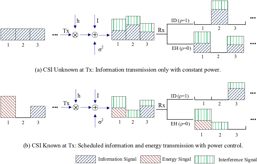
First, consider the case of CSI Unknown at Tx. As shown in Fig. 2(a), in this case Tx transmits information continuously with constant power for all the fading states due to the lack of CSIT. At each fading state , Rx decides whether to decode the information or harvest the energy from the received signal based on and . For example, as shown in Fig. 2(a), time slots 1 and 3 are switched to EH mode at Rx, while time slot 2 is switched to ID mode. For convenience, we define an indicator function to denote the receiver’s mode switching at any given as follows:
Next, we consider the case of CSI Known at Tx, i.e., the channel gain and interference power are known at Tx for each fading state . In this case, Tx is able to schedule transmission for information and energy transfer to Rx based on the instantaneous CSI. As shown in Fig. 2(b), Tx allocates time slot 1 for energy transfer, time slot 3 for information transfer, and transmits no signals in time slot 2. Accordingly, Rx will be in EH mode (i.e., ) to harvest energy from the received signal (including the interference) in time slot 1 or solely from the received interference in time slot 2, but in ID mode (i.e., ) to decode the information in time slot 3. In addition to transmission scheduling, Tx can implement power control based on the CSI to further improve the information/energy transmission efficiency. Let denote the transmit power of Tx at fading state . In this paper, we consider two types of power constraints on , namely average power constraint (APC) and peak power constraint (PPC) [15]. The APC limits the average transmit power of Tx over all the fading states, i.e., , where denotes the expectation over . In contrast, the PPC constrains the instantaneous transmit power of Tx at each of the fading states, i.e., , . Without loss of generality, we assume . For convenience, we define the set of feasible power allocation as
| (3) |
III Information Transfer and Energy Harvesting Trade-offs in Fading Channels
In this paper, we consider three performance measures at Rx, which are the outage probability and the ergodic capacity for wireless information transfer and the average harvested energy for WEH. For delay-limited information transmission, outage probability is a relevant performance indicator. Assuming that the interference is treated as additive Gaussian noise at Rx and the transmitted signal is Gaussian distributed, the instantaneous mutual information (IMI) for the Tx-Rx link at fading state is expressed as
| (4) |
Note that if Rx switches to EH mode (i.e., . Thus, considering a delay-limited transmission with constant rate , following [17] the outage probability at Rx can be expressed as
| (5) |
where denotes the probability. For information transfer without CSIT, the receiver-aware outage probability is usually minimized with a constant transmit power, i.e., , [17], whereas in the case with CSIT, the transmitter-aware outage probability can be further minimized with the “truncated channel inversion” based power allocation [18], [19].
Next, consider the case of no-delay-limited information transmission for which the ergodic capacity is a suitable performance measure expressed as
| (6) |
For information transfer, if CSIT is not available, the ergodic capacity can be achieved by a random Gaussian codebook with constant transmit power over all different fading states [20]; however, with CSIT, the ergodic capacity can be further maximized by the “water-filling” based power allocation [19].
On the other hand, the amount of energy (normalized to the transmission block duration) that can be harvested at Rx at fading state is expressed as , where is a constant that accounts for the loss in the energy transducer for converting the harvested energy to electrical energy to be stored; for convenience, it is assumed that in this paper. Moreover, since the background thermal noise has constant power for all the fading states and is typically a very small amount for energy harvesting, we may ignore it in the expression of . Thus, in the rest of this paper, we assume
| (7) |
The average energy that can be harvested at Rx is then given by
| (8) |
It is easy to see that there exist non-trivial trade-offs in assigning the receiver mode and/or transmit power (in the case of CSIT) to balance between minimizing the outage probability or maximizing the ergodic capacity for information transfer versus maximizing the average harvested energy for WEH. To characterize such trade-offs, for the case when information transmission is delay-limited, we introduce a so-called Outage-Energy (O-E) region (defined below) that consists of all the achievable non-outage probability (defined as with outage probability given in (5)) and average harvested energy pairs for a given set of transmit power constraints, while for the case when information transmission is not delay-limited, we use another Rate-Energy (R-E) region (defined below) that consists of all the achievable ergodic capacity and average harvested energy pairs. More specifically, in the case without (w/o) CSIT, the corresponding O-E region is defined as
| (9) |
while in the case with CSIT, the O-E region is defined as
| (10) |
On the other side, in the case without CSIT, the R-E region is defined as
| (11) |
while in the case with CSIT, the R-E region is defined as
| (12) |


Fig. 3(a) and Fig. 3(b) show examples of the O-E region without or with CSIT (see Sections IV-A and IV-B for the details of computing the O-E regions for these two cases) and the R-E region without or with CSIT (see Sections V-A and V-B for the corresponding details), respectively. It is assumed that , , , , and are independent exponentially distributed RVs with mean and , respectively. It is observed that CSIT helps improve both the achievable outage-energy and rate-energy trade-offs.
It is observed from Fig. 3 that in each region, there are two boundary points that indicate the extreme performance limits, namely, and for the O-E region, or and for the R-E region. For brevity, characterizations of these vertex points are given in Appendix.
Since the optimal trade-offs between the non-outage probability/ergodic capacity and the average harvested energy are characterized by the boundary of the corresponding O-E/R-E region, it is important to characterize all the boundary or pairs in each case with or without CSIT. From Fig. 3, it is easy to observe that if , the non-outage probability or ergodic capacity can still be achieved for both cases with and without CSIT. Thus, the remaining boundary of the O-E region yet to be characterized is over the intervals and , while that of the R-E region is over the intervals and .
For the O-E region, we introduce the following indicator function for the event of non-outage transmission at fading state for the convenience of our subsequent analysis:
It thus follows that the non-outage probability can be reformulated as
| (15) |
Then, we consider the following two optimization problems.
where is a target average harvested energy required to maintain the receiver’s operation. By solving Problem (P1) or (P2) for all , we are able to characterize the entire boundary of the O-E region for the case without CSIT (defined in (9)) or with CSIT (defined in (10)).
Similarly, for the R-E region, we consider the following two optimization problems.
Then, by solving Problem (P3) or (P4) for all , we can characterize the boundary of the R-E region for the case without CSIT (defined in (11)) or with CSIT (defined in (12)).
It is observed that the objective function of Problem (P2) is in general not concave in even if ’s are given. Furthermore, due to the integer constraint , , Problems (P1)-(P4) are in general non-convex optimization problems. However, it can be verified that all of them satisfy the “time-sharing” condition given in [21]. To show this for Problem (P1), let denote the optimal problem value given the harvested energy constraint , and and denote the optimal solutions given the harvested energy constraints and , respectively. We need to prove that for any , there always exists at least one solution such that and , where and is defined accordingly as in (III). Due to the space limitation, the above proof is omitted here. In fact, the “time-sharing” condition implies that is concave in , which then guarantees the zero duality gap for Problem (P1) according to the convex analysis in [22]. Similarly, it can be shown that strong duality holds for Problems (P2)-(P4). Therefore, in the following two sections, we apply the Lagrange duality method to solve Problems (P1)-(P4) to obtain the optimal O-E and R-E trade-offs, respectively.
IV Outage-Energy Trade-off
In this section, we study the optimal receiver mode switching without/with transmit power control to achieve different trade-offs between the minimum outage probability and the maximum average harvested energy for both cases without and with CSIT by solving Problems (P1) and (P2), respectively.
IV-A The Case Without CSIT: Optimal Receiver Mode Switching
We first study Problem (P1) for the CSIT-unknown case to derive the optimal rule at Rx to switch between EH and ID modes. The Lagrangian of Problem (P1) is formulated as
| (16) |
where is the dual variable associated with the harvested energy constraint . Then, the Lagrange dual function of Problem (P1) is expressed as
| (17) |
The maximization problem (17) can be decoupled into parallel subproblems all having the same structure and each for one fading state. For a particular fading state , the associated subproblem is expressed as
| (18) |
where . Note that we have dropped the index for the fading state for brevity.
To solve Problem (18), we need to compare the values of for and . It follows from (7), (III) and (16) that when ,
and when ,
| (21) |
Thus, the optimal solution to Problem (18) is obtained as
With a given , Problem (17) can be efficiently solved by solving Problem (18) for different fading states. Problem (P1) is then solved by iteratively solving Problem (17) with a fixed , and updating via a simple bisection method until the harvested energy constraint is met with equality [23].
Next, we examine the optimal solution to Problem (P1) to gain more insights to the optimal receiver mode switching in the case without CSIT. With a given harvested energy constraint , we define the region on the plane consisting of all the points for which the optimal solution to Problem (P1) is (versus ) as the optimal ID region (versus the optimal EH region). Furthermore, let denote the optimal dual solution to Problem (P1) corresponding to the given . Then, from (V-A) the optimal ID region for Problem (P1) is expressed as
| (24) |
The rest of the non-negative plane is thus the optimal EH region, i.e.,
| (25) |
where denotes the two-dimensional nonnegative real domain, and denotes the set .

An illustration of and is shown in Fig. 4 with . It is noted that to meet the harvested energy constraint , we need to sacrifice (increase) the outage probability for information transfer by allocating some non-outage fading states in the region to EH mode. An interesting question here is to decide which portion of should be allocated to EH mode. It is observed from Fig. 4 that the optimal way is to allocate all pairs satisfying or in to EH mode, i.e., the fading states with sufficiently large signal plus interference total power values at Rx should be allocated to EH mode. This is reasonable since if we have to allocate a certain number of fading states in to EH mode, i.e., increase the transmission outage probability by the same amount, these fading states should be chosen to maximize the harvested energy at Rx.
Furthermore, note that increases monotonically with . Thus, the boundary line that separates the optimal ID and EH regions in Fig. 4 will be shifted down as increases, and as a result shrinks. It can be shown that if , then , which corresponds to the point of the O-E region shown in Fig. 3(a) for the case without CSIT.
It is worth noting that if , , then the optimal ID region reduces to , and the rest of the -axis is thus the EH region. In this case, the outage fading states are all allocated to EH mode since they cannot be used by ID mode. However, the harvested energy in the outage states only accounts for a small portion of the total harvested energy due to the poor channel gains. Most of the energy is harvested in the interval , i.e., when the channel power is above a certain threshold.
IV-B The Case With CSIT: Joint Information/Energy Scheduling, Power Control, and Receiver Mode Switching
In this subsection, we address the case of CSI known at Tx and jointly optimize the energy/information scheduling and power control at Tx, as well as EH/ID mode switching at Rx, as formulated in Problem (P2). Let and denote the nonnegative dual variables corresponding to the average harvested energy constraint and average transmit power constraint, respectively. Similarly as for Problem (P1), Problem (P2) can be decoupled into parallel subproblems each for one particular fading state and expressed as (by ignoring the fading index )
| (26) |
where . To solve Problem (26), we need to compare the optimal values of for and , respectively, as shown next.
When , it follows that
where . It can be verified that the optimal power allocation for the ID mode to maximize (IV-B) subject to is the well-known “truncated channel inversion” policy [19] given by
where .
When , it follows that
| (31) |
Define . Then the optimal power allocation for the EH mode can be expressed as
To summarize, we have
Then, given any pair of and , the optimal solution to Problem (26) for fading state can be expressed as
Next, to find the optimal dual variables and for Problem (P2), sub-gradient based methods such as the ellipsoid method [23] can be applied. It can be shown that the sub-gradient for updating is , where and denote the harvested energy and transmit power at fading state , respectively, after solving Problem (26) for a given pair of and . Hence, Problem (P2) is solved.
Next, we investigate further the optimal information/energy transfer scheduling and power control at Tx, as well as the optimal mode switching at Rx. For simplicity, we only study the case of , . From the above analysis, it follows that there are three possible transmission modes at Tx for the case with CSIT: “information transfer mode” with channel inversion power control, “energy transfer mode” with peak transmit power, and “silent mode” with no transmission, where the first transmission mode corresponds to ID mode at Rx and the second transmission mode corresponds to EH mode at Rx. We thus define , , and on the non-negative -axis as the regions corresponding to the above three modes, respectively. Since the explicit expressions for characterizing these regions are complicated and depend on the values of and , in the following we will study , , and in the special case of to shed some light on the optimal design. Let and denote the optimal dual solutions to Problem (P2). With , it can be shown that , and , where is the largest root of the equation: . The proof is omitted here due to the space limitation.
An illustration of , , and for the case of , , and is shown in Fig.5. Similar to the case without CSIT (cf. Fig. 4), the optimal design for the case with CSIT is still to allocate the best channels to the EH mode rather than the ID mode. However, unlike the case without CSIT, when the channel condition is poor, the transmitter in the case with CSIT will shut down its transmission to save power.

V Rate-Energy Trade-off
In this section, we investigate the optimal resource allocation schemes to achieve different trade-offs between the maximum ergodic capacity and maximum averaged harvested energy for the two cases without and with CSIT by solving Problems (P3) and (P4), respectively.
V-A The Case Without CSIT: Optimal Receiver Mode Switching
First, we study Problem (P3) for the CSIT-unknown case to derive the optimal switching rule at Rx between EH and ID modes for characterizing different R-E trade-offs. Similarly as in Section IV-A, Problem (P3) can be decoupled into parallel subproblems each for one particular fading state , expressed as
| (44) |
where with denoting the dual variable associated with the harvested energy constraint . Note that we have dropped the index of the fading state for brevity.
To solve Problem (44), we need to compare the values of for and . When , it follows that
| (45) |
When , it follows that
| (46) |
Thus, the optimal solution to Problem (44) is obtained as
To find the optimal dual variable to Problem (P3), a simple bisection method can be applied until the harvested energy constraint is met with equality. Thus, Problem (P3) is efficiently solved.
Similar to Section IV-A, in the following we characterize the optimal ID region and EH region to get more insights to the optimal receiver mode switching for characterizing different R-E trade-offs. Let denote the optimal dual variable corresponding to a given energy target . The optimal ID region can then be expressed as
| (49) |
The rest of the non-negative plane is thus the optimal EH region, i.e.,
| (50) |
Define . Fig. 6 gives an illustration of the optimal ID region and EH region for a particular value of .

Next, we discuss the optimal mode switching rule at Rx for achieving various R-E trade-offs in the case without CSIT. Similar to the case of O-E trade-off, for meeting the harvested energy constraint , we need to sacrifice (decrease) the ergodic capacity for information transfer by allocating some fading states to EH mode. Similar to the discussions in Section IV, the optimal rule is to allocate fading states with largest values of for information transfer to EH mode. The reason is that although fading states with good direct channel gains are most desirable for ID mode, from (45) and (46) it is observed that the Lagrangian value of ID mode increases logarithmically with , while that of EH mode increases linearly with . As a result, when is above a certain threshold, the value of will be larger than that of . In other words, when is good enough, we can gain more by switching from ID mode to EH mode.
It is also observed that as the value of increases, the optimal ID region shrinks. In the following, we derive the value of corresponding to the point in Fig. 3(b). From Fig. 6 it can be observed that has two intersection points with the -axis, one of which is . It can be shown that is a monotonically increasing function of in the interval , and decreasing function of in the interval . Consequently, if , i.e., , the other intersection point of with the -axis will coincide with the point , and thus if .
V-B The Case With CSIT: Joint Information/Energy Scheduling, Power Control, and Receiver Mode Switching
In this subsection, we study Problem (P4) to achieve different optimal R-E trade-offs for the case of CSIT by jointly optimizing energy/information scheduling and power control at Tx, together with the EH/ID mode switching at Rx. For Problem (P4), let and denote the nonnegative dual variables corresponding to the average harvested energy constraint and average transmit power constraint, respectively. Then, Problem (P4) can be decoupled into parallel subproblems each for one particular fading state and expressed as (by ignoring the fading index )
| (51) |
where . To solve Problem (51), we need to compare the maximum values of for and , respectively, as shown next.
When , it follows that
| (52) |
It can be shown that the optimal power allocation for this case is the well-known “water-filling” policy [19]. Let . The optimal power allocation for information transfer can be expressed as
| (53) |
where .
When , it follows that has the same expression as that given in (31), and consequently, the optimal power allocation for EH mode, , is given by (IV-B).
To summarize, for ID mode, if , we have
If , we have
For EH mode, the expression of is the same as that given in (IV-B).
Then, given a pair of and , the optimal solution to Problem (51) for fading state can be expressed as
Next, to find the optimal dual variables and for Problem (P4), similarly as in Section IV-B, the ellipsoid method can be applied. Thus, Problem (P4) is efficiently solved.
Next, we investigate further the optimal information/energy transfer scheduling and power control at Tx, as well as the optimal mode switching rule at Rx. For simplicity, we only consider the case of , . Since there is no interference, it can be observed from (V-B) and (V-B) that there are three possible transmission modes at Tx for the case with CSIT: “information transfer mode” with water-filling power control, “energy transfer mode” with peak transmit power, and “silent mode” with no transmission, where the first transmission mode corresponds to ID mode at Rx and the second transmission mode corresponds to EH mode at Rx. Similar to the analysis in Section IV-B, we can define , , and on the non-negative -axis as the regions corresponding to the above three modes, respectively. Let and denote the optimal dual solutions to Problem (P4). For brevity, in the following we only present the expressions of the above regions in the case of . It can be shown that in this case, , and , where is the largest root of the equation: , which can be obtained by the bisection method over the interval . The proof is omitted here due to the space limitation.
An illustration of , , and in the case without interference and is given in Fig. 7. Compared with the case without CSIT (cf. Fig. 6), it can be similarly observed that the channels with largest power are allocated to EH mode. However, when the channel condition is very poor, the transmitter will shut down its transmission to save power in the case with CSIT, instead of transmitting constant power in the case without CSIT.

VI Consideration of Receiver Energy Consumption
In the above analysis, we have ignored energy consumptions at the receiver for the purpose of exposition. In this section, we extend the result by considering the receiver energy consumption. Firstly, we explain in more details the operations of the receiver in each block and their corresponding energy consumptions as follows. At the beginning of each block, the receiver estimates the channel and interference power gains to determine which of the EH/ID mode it will switch to, where we assume a constant energy being consumed. After that, suppose the receiver switches to EH mode. Since practical energy receivers are mostly passive [6], we assume that the energy consumed by the energy receiver is negligibly small and thus can be ignored. However, if the receiver switches to ID mode, more substantial energy consumption is required [6]; for simplicity, we assume that a constant power incurs due to the information receiver when it is switched on. In the following, we will study the effect of the above receiver power consumptions on the optimal operation of the time-switching receiver. Due to the space limitation, we will only study the O-E trade-off in the case without CSIT, while similar results can be obtained for other cases.
Let denote the receiver power consumption due to ID mode at fading state , and denote the net harvested energy obtained by subtracting and from the harvested energy . To study the O-E trade-off in the case without CSIT, we modify Problem (P1) as
Since is a constant for all fading states, without loss of generality we absorb this term into and assume in the rest of this paper for convenience.
Let denote the optimal dual variable corresponding to the net harvested energy constraint. We then solve Problem (P5) in a similar way as for Problem (P1). The optimal solution of Problem (P5) can be expressed as
As a result, the optima ID region when the receiver energy consumption is considered can be defined as
| (67) |
and the rest of the plane is the optimal EH region. An illustration of the optimal ID region and EH region is given in Fig. 8. By comparing it with Fig. 4 for the case without considering the receiver energy consumption, we observe that to harvest the same amount of net energy we need to allocate more fading states in (24) to EH mode, i.e., allocating all pairs satisfying to EH mode with .


Fig. 9 shows an example of the O-E region without CSIT but considering the receiver power consumption. The setup is the same as that for Fig. 3. It is observed that the receiver power consumption degrades the O-E trade-off. However, does not change the value because it is achieved when all the fading states are allocated to EH mode and thus has no effects. Moreover, it is observed that when , the same maximum non-outage probability as that of the case without receiver energy consumption (i.e., ) is achieved, while when , a smaller is achieved. The reason is as follows. If is not large enough, the energy harvested in the outage fading states can offset the receiver power consumption in the non-outage fading states. As a result, all the non-outage fading states can still be allocated to ID mode. Otherwise, if is too large, then we have to sacrifice some non-outage fading states to EH mode to harvest more energy for ID mode, and thus the value of is reduced.
VII Numerical Results
In this section, we evaluate the performance of the proposed optimal schemes as compared to three suboptimal schemes (to be given later) that are designed to reduce the complexity at Rx and thus yields suboptimal O-E or R-E trade-offs. We assume that Rx needs to have an average harvested energy to maintain its normal operation. Thus, with a given , we will compute and then compare the minimum outage probability or the maximum ergodic capacity achievable by the optimal and suboptimal schemes.
First, we introduce three suboptimal receiver mode switching rules, namely, Periodic Switching, Interference-Based Switching, and SINR-Based Switching as follows.
- •
Periodic Switching: In this scheme, Rx switches between ID mode and EH mode periodically regardless of the CSI. For convenience, let with denote the portion of time switched to EH mode; then denotes the portion of time for ID mode. The value of is determined such that the given energy constraint is satisfied. For example, for the O-E trade-off without CSIT, the maximum harvested energy is given in (69). Thus, can be obtained as . For other trade-off cases, can be obtained similarly.
- •
Interference-Based Switching: In this scheme, we assume that Rx’s mode switching is determined solely by the interference power . When where denotes a preassigned threshold, Rx switches to EH mode; otherwise, it switches to ID mode. The value of is determined so as to meet the given energy constraint , and the derivation of ’s for different trade-off cases are omitted for brevity.
- •
SINR-Based Switching: In this scheme, the mode switching is based on the receiver’s signal-to-noise-plus-interference ratio (SINR) . If where denotes a predesigned SINR threshold, Rx switches to ID mode; otherwise, it switches to EH mode. The value of is determined so as to meet the given energy constraint , while the derivation of ’s for different trade-off cases are omitted due to the space limitation.
Moreover, if CSIT is available, Tx can implement the optimal power control to minimize the outage probability or maximize the ergodic capacity for information transfer, according to each of the above three suboptimal Rx’s mode switching rules.


Next, we show the performance comparison of the three suboptimal schemes with the optimal scheme given in Section IV-A for delay-limited transmission without CSIT and that given in Section V-B for no-delay-limited transmission with CSIT in Figs. 10 and 11, respectively. The setup is as follows. The PPC is , the noise power is , and for the O-E case, the constant rate requirement is . We further assume that and are independent exponentially distributed RVs with mean and , respectively. In addition, the energy target at Rx is set to be .
Fig. 10 shows the achievable minimum outage probability of different schemes with given for the delay-limited information transmission without CSIT. It is observed that in general the interference-based switching works pretty well since its performance is similar to that of the optimal switching derived in Section IV-A for all values of with only a small gap. On the contrary, the periodic switching rule does not perform well with an outage probability loss of about as compared to the optimal switching.
Another interesting observation is on the performance of the SINR-based switching. It is observed from Fig. 10 that when , the performance of SINR-based switching is the same as that of the optimal switching. However, as increases, its performance degrades. When , its achievable outage probability is even higher than that of periodic switching. The above observations can be explained as follows. It can be seen from (70) in Appendix that if we view as a function of , the following trade-off arises: if the value of is larger, less number of fading states are allocated to EH mode, but more energy are harvested in each fading state allocated to EH mode. To analyze the behavior of over , for the case with and , we can derive an explicit expression of as follows:
| (68) |
It can be shown that in our setup (, , and ), is a monotonically decreasing function with respect to when . Moreover, when , . Thus, if , it follows that . In other words, if , the minimum outage probability with harvested energy constraint is achieved when Rx switches to ID mode in the fading states and switches to EH mode in any subset of to meet the energy constraint. Consequently, the SINR-based switching is optimal when is small. When , the minimum harvested energy cannot meet the energy constraint, and as shown in Section IV-A, the optimal switching is to allocate some fading states with the largest value of in to EH mode. However, the SINR-based switching does the opposite way: it tends to allocate the fading states with small value of to EH mode. Thus, when is large and a certain number of fading states are allocated to EH mode, the incremental harvested energy by the SINR-based switching is far from that by the optimal switching. To recover this energy loss, more fading states need to be allocated to EH mode. This is why the SINR-based switching results in very high outage probability when becomes large.
Fig. 11 shows the achievable maximum rate of different schemes with given for the no-delay-limited information transmission with CSIT. Similar to Fig. 10, it is observed from Fig. 11 that the performance of the interference-based switching is very close to that of the optimal switching derived in Section V-B, while the performances of the other two suboptimal switching rules are notably worse. Under certain conditions (e.g., when SNRdB in Fig. 11), the performance of the SINR-based switching can be even worse than that of the periodic switching. This is as expected since although high SINR is preferred by information decoding, the optimal mode switching rule derived in Section V-B is determined by both the values of and , but has no direct relationship to the ratio of them, i.e., the SINR value. Thus, the performance of the SINR-based switching cannot be guaranteed.
VIII Concluding Remarks
This paper studied an emerging application in wireless communication where the receiver opportunistically harvests the energy from the unintended interference and/or intended signal in addition to decoding the information. Under a point-to-point flat-fading channel setup with time-varying interference, we derived the optimal ID/EH mode switching rules at the receiver to optimize the outage probability/ergodic capacity versus harvested energy trade-offs. When the CSI is known at the transmitter, joint optimization of transmitter information/energy scheduling and power control with the receiver ID/EH mode switching was also investigated. Somehow counter-intuitively, we showed that for wireless information transfer with opportunistic energy harvesting, the best strategy to achieve the optimal O-E and R-E trade-offs is to allocate the fading states with the best direct channel gains to power transfer rather than information transfer. Moreover, three heuristic mode switching rules were proposed to reduce the complexity at Rx, and their performances were compared against the optimal performance.
There are important problems unaddressed yet in this paper and thus worth further investigation, some of which are highlighted as follows:
- •
In this paper, we assumed that the interference is within the same band as the transmitted signal from Tx. As a result, the algorithms proposed in this paper to achieve the optimal O-E or R-E trade-offs cannot be directly applied to the case of wide-band interference. It is thus interesting to investigate how to manage the wide-band interference in a wireless energy harvesting communication system.
- •
In this paper, we studied the optimal mode switching and/or power control rules in a single-user setup subject to an aggregate interference at the receiver. However, how to extend the results of this paper to the multi-user setup is an unsolved problem. For the multi-user interference channel, interference management is a key issue. Traditionally, interference is either decoded and subtracted when it is strong or treated as noise when it is weak. In this paper, we provide a new approach to deal with the interference by utilizing it as a new source for energy harvesting. Thus, how should the Tx-Rx links in an interference channel cooperate with each other to manage the interference by optimally balancing between information and power transfer is an intricate problem requiring further investigation.
In this appendix, we characterize the vertex points on the boundary of the O-E region and R-E region (cf. Fig. 3) for both the cases with and without CSIT.
-1 O-E region without CSIT
As shown in Fig. 3(a), is given by
| (69) |
when , , i.e., EH mode is active all the time at Rx and thus the resulting non-outage probability (corresponding to the outage probability equal to 1). Moreover, and are given by
| (70) | ||||
| (71) |
Note that is the minimum average harvested energy at Rx when the maximum non-outage probability (or minimum outage probability) is achieved. Since the set for the outage fading states is non-empty in (70), in general.
-2 O-E region with CSIT
As shown in Fig. 3(a), the point is achieved when all the fading states are allocated to EH mode, i.e., , . Thus, the resulting non-outage probability is . Moreover, the harvested energy can be expressed as , where the first term is the energy harvested from the signal, while the second term is due to the interference. To maximize the first term under both the PPC and APC, the optimal power control policy is to transmit at peak power at the fading states with the largest possible ’s. Let be the threshold that satisfies
| (72) |
Then can be expressed as
| (73) |
To obtain , we need to minimize the outage probability under both the APC and PPC without presence of the energy harvester. It can be shown that the optimal power allocation to achieve the maximum non-outage probability can be expressed as the well-known truncated channel inversion policy [18], [19]:
where with denoting the optimal dual variable associated with the APC that satisfies . Then the maximum non-outage can be expressed as
| (76) |
On the other hand, is achieved when Rx harvests energy at all the outage fading states. Let denote the value of that satisfies
| (77) |
Then the minimum harvested energy can be expressed as
| (78) |
Note that if , then , i.e., no power is available for energy transfer at Tx. Thus, is only due to the interference power. Since the set for the outage fading states is non-empty, since the receiver can at least harvest energy from the interference in the outage fading states.
-3 R-E region without CSIT
As shown in Fig. 3(b), the maximum harvested energy is achieved when all the fading states are allocated to EH mode, i.e., , , and thus has the same expression as that given in (69). Moreover, . On the other hand, the ergodic capacity is maximized when all the fading states are allocated to ID mode, i.e., , . Consequently, and
| (79) |
-4 R-E region with CSIT
As shown in Fig. 3(b), similar to the case of O-E region with CSIT, the maximum harvested energy is given in (73), and . As for the point , to maximize the ergodic capacity under both the APC and PPC, the optimal transmit power policy is the well-known “water-filling“ power allocation given by [19]
| (80) |
where , and is the optimal dual variable associated with satisfying . Thus, the maximum rate is given by
| (81) |
Then, for the fading states satisfying , Rx can harvest energy from the interference. Thus the minimum harvested energy is in general non-zero and can be expressed as
| (82) |
References
- [1] S. Sudevalayam and P. Kulkarni, “Energy harvesting sensor nodes: survey and implications,” IEEE Commun. Surveys Tuts., vol. 13, no. 3, pp. 443-461, 2011.
- [2] L. R. Varshney, “Transporting information and energy simultaneously,” in Proc. IEEE Int. Symp. Inf. Theory (ISIT), pp. 1612-1616, July 2008.
- [3] P. Grover and A. Sahai, “Shannon meets Tesla: wireless information and power transfer,” in Proc. IEEE Int. Symp. Inf. Theory (ISIT), pp. 2363-2367, June 2010.
- [4] R. Zhang and C. K. Ho, “MIMO broadcasting for simultaneous wireless information and power transfer,” submitted for publication. (Available online at arXiv:1105.4999)
- [5] L. R. Varshney, ”Unreliable and resource-constrained decoding,” Ph.D Thesis, EECS Department, MIT, June 2010.
- [6] X. Zhou, R. Zhang, and C. Ho, “Wireless information and power transfer: architecture design and rate-energy tradeoff,” to appear in IEEE Globecom, 2012. (Available online at arXiv:1205.0618).
- [7] T. Han and K. Kobayashi, “A new achievable rate region for the interference channel,” IEEE Trans. Inf. Theory, vol. 27, pp. 49-60, Jan. 1981.
- [8] X. Shang, G. Kramer, and B. Chen, “A new outer bound and the noisy-interference sum-rate capacity for Gaussian interference channels,” IEEE Trans. Inf. Theory, vol. 55, no. 2, pp. 689-699, Feb. 2009.
- [9] V. Annapureddy and V. Veeravalli, “Gaussian interference networks: sum capacity in the low interference regime and new outer bounds on the capacity region,” IEEE Trans. Inf. Theory, vol. 55, no. 7, pp. 3032-3050, July 2009.
- [10] V. R. Cadambe and S. A. Jafar, “Interference alignment and degrees of freedom of the K-user interference channel,” IEEE Trans. Inf. Theory, vol. 54, no. 8, pp. 3425-3441, Aug. 2008.
- [11] C. K. Ho and R. Zhang, “Optimal energy allocation for wireless communications with energy harvesting constraints,” IEEE Trans. Sig. Process., vol. 60. no. 9, pp. 4808-4818, Sep. 2012.
- [12] R. Rajesh, V. Sharma, and P. Viswanath, “Capaciy of fading Gaussian channel with an energy harvesting sensor node,” in Proc. Global Commun. Conf. (Globecom), Dec. 2011.
- [13] V. Sharma, U. Mukherji, V. Joseph, and S. Gupta., “Optimal energy management policies for energy harvesting sensor nodes,” IEEE Trans. Wireless Commun., vol. 9, no. 4, pp. 1326-1336, Apr. 2010.
- [14] O. Ozel, K. Tutuncuoglu, J. Yang, S. Ulukus, and A. Yener, “Transmission with energy harvesting nodes in fading wireless channels: optimal policies,” IEEE J. Sel. Area Commun., vol. 29, no. 8, pp. 1732-1743, Sep. 2011.
- [15] E. Biglieri, J. Proakis, and S. Shamai (Shitz), “Fading channels: information-theoretic and communications aspects,” IEEE Trans. Inf. Theory, vol. 44, no. 6, pp. 2619-2692, Oct. 1998.
- [16] R. J. McEliece and W. E. Stark, “Channels with block interference,” IEEE Trans. Inf. Theory, vol. 30, pp. 44-53, Jan. 1984.
- [17] L. H. Ozarow, S. Shamai, and A. D. Wyner, “Information theoretic considerations for cellular mobile radio,” IEEE Trans. Veh. Technol., vol. 43 no. 2, pp. 359-378, 1994.
- [18] G. Caire, G. Taricco, and E. Biglieri, “Optimal power control over fading channels,” IEEE Trans. Inf. Theory, vol. 45, no. 5, pp. 1468-1489, Jul. 1999.
- [19] A. Goldsmith and P. P. Varaiya, “Capacity of fading channels with channel side information,” IEEE Trans. Inf. Theory, vol. 43, no. 6, pp. 1986-1992, Nov. 1997.
- [20] G. Caire and S. Shamai (Shitz), “On the capacity of some channels with channel state information,” IEEE Trans. Inf. Theory, vol. 45, no. 6, pp. 2007-2019, Sep. 1999.
- [21] W. Yu and R. Lui, “Dual methods for nonconvex spectrum optimization of multicarrier systems,” IEEE Trans. Commun., vol. 54, no. 7, pp. 1310-1322, July 2006.
- [22] R. T. Rockafellar, Convex Analysis, Princeton Univ. Press, 1970.
- [23] S. Boyd and L. Vandenberghe, Convex Optimization, Cambidge Univ. Press, 2004.