Multi-intersection Traffic Light Control Using Infinitesimal Perturbation Analysisfootnoteinfo
Abstract
We address the traffic light control problem for multiple intersections in tandem by viewing it as a stochastic hybrid system and developing a Stochastic Flow Model (SFM) for it. Using Infinitesimal Perturbation Analysis (IPA), we derive on-line gradient estimates of a cost metric with respect to the controllable green and red cycle lengths. The IPA estimators obtained require counting traffic light switchings and estimating car flow rates only when specific events occur. The estimators are used to iteratively adjust light cycle lengths to improve performance and, in conjunction with a standard gradient-based algorithm, to obtain optimal values which adapt to changing traffic conditions. Simulation results are included to illustrate the approach.
keywords
Traffic Light Control, SFM, IPA.1 Introduction
The Traffic Light Control (TLC) problem aims at dynamically controlling the flow of traffic at an intersection through the timing of green/red light cycles with the objective of reducing congestion, hence also the delays incurred by drivers. The more general problem involves a set of intersections and traffic lights with the objective of reducing overall congestion over an area covering multiple urban blocks. Since the control of one intersection influences the traffic flow from or towards others, this is a complex problem further complicated by the fact that traffic flows constantly change depending on the time of day, accidents, weather conditions, etc. Recent technological developments involving better, inexpensive sensors and wireless sensor networks have enabled the collection of data (e.g., counting vehicles in a specific road section) which can be used to optimally select traffic light cycles over specific time intervals in a day or even to dynamically control them based on real-time data. Thus, methodologies that would not be possible to implement not long ago are now becoming feasible. The approach proposed in this paper to the TLC problem is specifically intended to exploit these recent developments.
Several different approaches have been proposed to solve the TLC problem. It is formulated as a Mixed Integer Linear Programming (MILP) problem in Dujardin et al. (2011), and as an Extended Linear Complementary Problem (ELCP) in DeSchutter (1999). A Markov Decision Process (MDP) approach has been proposed in Yu and Recker (2006) and Reinforcement Learning (RL) was used in Thorpe (1997), with several extensions found in Prashanth and Bhatnagar (2011); Wiering et al. (2004). A game theoretic viewpoint is given in Alvarez and Poznyak (2010), while a hybrid system formulation is presented in Zhao and Chen (2003). Due to its complexity when viewed as an optimization problem, fuzzy logic is often used in both a single (isolated) junction Murat and Gedizlioglu (2005) and multiple junctions Choi et al. (2002). Expert systems Findler and Stapp (1992) and evolutionary algorithms Taale et al. (1998) have also been applied to develop a traffic light controller for a single intersection. Perturbation analysis techniques were used in Head et al. (1996) and a formal approach using Infinitesimal Perturbation Analysis (IPA) to solve the TLC problem was presented in Panayiotou et al. (2005) for a single intersection.
In Geng and Cassandras (2012), we study the TLC problem for a single intersection using a Stochastic Flow Model (SFM) and Infinitesimal Perturbation Analysis (IPA). In this paper, we extend our analysis to two tandem intersections. We still adopt a stochastic hybrid system modeling framework (see Cassandras and Lafortune (2008),Cassandras and Lygeros (2006)), since the problem involves both event-driven dynamics in the switching of traffic lights and time-driven dynamics that capture the flow of vehicles through an intersection. Although one can also view this as a purely Discrete Event System (DES) with the intersection area as a “server” processing “users” (vehicles), the fact that a vehicle does not exclusively occupy this area makes a flow-based viewpoint a more accurate way to model such a process. While in most traditional flow models the flow rates involved are treated as deterministic parameters, a SFM as introduced in Cassandras et al. (2002) treats them as stochastic processes. In the TLC problem, this is consistent with continuously and randomly varying traffic flows, especially in heavy traffic conditions where the problem is most interesting. With only minor technical assumptions imposed on the properties of such processes, a general IPA theory for stochastic hybrid systems was recently presented in Wardi et al. (2010),Cassandras et al. (2010) through which one can estimate on line gradients of certain performance measures with respect to various controllable parameters. These estimates may be incorporated in standard gradient-based algorithms to optimize system parameter settings. IPA was originally developed as a technique for evaluating gradients of sample performance functions in queueing systems and using them as unbiased gradient estimates of performance metrics. However, IPA estimates become biased when dealing with aspects of queueing systems such as multiple user classes, blocking due to limited resource capacities, and various forms of feedback control. The use of IPA in stochastic hybrid systems, however, circumvents these limitations and yields simple unbiased gradient estimates (under mild technical conditions) of useful metrics even in the presence of blocking and a variety of feedback control mechanisms (see Yao and Cassandras (2011a).)
In Section 2, we formulate the TLC problem for two intersections and construct a SFM. In Section 3, we derive an IPA estimator for a cost function gradient with respect to a controllable parameter vector defined by green and red cycle lengths. This is then used to iteratively adjust these cycle lengths to improve performance and, under proper conditions, obtain optimal parameter values. Simulation-based examples are given in Section 4 and we conclude with Section 5.
2 Problem Formulation
In this paper, we concentrate on solving the TLC problem for two coupled intersections, as shown in Fig. 1. There are four roads and four traffic lights, with each traffic light controlling the associated incoming traffic flow. The traffic in road 1 of intersection flows into road 3 of . For simplicity, we make the following assumptions: Left-turn and right-turn traffic flows are not considered, i.e., traffic lights only control vehicles going straight. A YELLOW light is combined with a RED light (therefore, the YELLOW light duration is not explicitly controlled). Road 3 is long enough that cars accumulated in it do not influence the departure process of road 1.

The system involves a number of stochastic processes which are all defined on a common probability space . Each of the four roads is considered as a queue with a random arrival flow process , where is the instantaneous vehicle arrival rate at time . When the traffic light corresponding to road is GREEN, the departure flow process is denoted by Let the GREEN light duration in a cycle of queue be , and the controllable parameter vector of interest is . We define a state vector where is the content of queue . We use the notation to emphasize the dependence of the queue content on ; however, for notational simplicity, we will write when no confusion arises. We also define a left-continuous “clock” state variable , , associated with the GREEN light cycle for queue as follows:
where is the index of the road perpendicular to road at the same intersection. We set . Thus, measures the time since the last switch from RED to GREEN of the traffic light for queue . It is reset to as soon as the GREEN cycle length is reached and remains at this value while the light is GREEN for queue ; as soon as that cycle ends, i.e., , then and the process repeats.
To simplify notation, we set if the Boolean expression used in (2), i.e., or , is true (light is GREEN) and otherwise. We can now write the dynamics of each state variable as follows:
| (3) |
where
| (4) |
In (4), describes the departure process if the road is not empty. According to assumption , is independent of . However, depends on the departure process of queue 1; in particular,
| (5) |
Combining (3) through (5), we have the dynamics of queue 3:
| (6) |
The operation of the intersection can be viewed as a hybrid system with the time-driven dynamics described by (3)-(6) and event-driven dynamics dictated by GREEN-RED light switches and by events causing some to switch from positive to zero or vice versa.

Using the standard definition of a Stochastic Hybrid Automaton (SHA) (e.g., see Cassandras and Lafortune (2008)), we may obtain a SHA model for queue 1,2 and 4 which is similar to Geng and Cassandras (2012). Here, we concentrate on the SHA for the operation of queue 3 as shown in Fig. 2. This reflects the fact that a typical sample path of any one of the queue contents (as shown in Fig. 3) consists of intervals over which , which we call Non-Empty Periods (NEPs), followed by intervals where , which we call Empty Periods (EPs). Thus, the entire sample path consists of a series of alternating NEPs and EPs. The event set that affects any queue is where is a switch in the sign of from non-positive to strictly positive, is a switch in the sign of from to strictly positive, is the queue content becoming empty, i.e., , which terminates a NEP (and initiates an EP), switches a light from RED to GREEN, and switches a light from GREEN to RED. For easier reference, we label as “” for the end of NEP events, as “” and as “” for the light switching events. The resulting start of a NEP is an event “induced” by either or or which we will refer to as an “” event. For queue 3, the event set includes all those events that cause a jump in the value of in (6). As we can see from Fig. 2, every event of also affects the dynamics of queue 3. Thus, we have .
Returning to Fig. 3, the th NEP in a sample path of queue 3, , is denoted by , i.e., , are the occurrence times of the th and event respectively at this queue. During the th NEP, , , denotes the time when an event occurs.
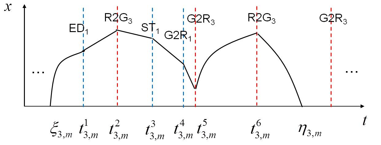

Our objective is to select so as to minimize a cost function that measures a weighted mean of the queue lengths over a fixed time interval . In particular, we define the sample function
| (7) |
where is a cost weight associated with queue and are given initial conditions. It is obvious that since during EPs of queue , we can rewrite (7) in the form
| (8) |
where is the total number of NEPs during the sample path of queue . For convenience, we also define
| (9) |
to be the sample cost associated with the th NEP of queue . We can now define our overall performance metric as
| (10) |
Since we do not impose any limitations on the processes and , it is infeasible to obtain a closed-form expression of . The only assumption we make is that , are piecewise continuous w.p. 1. The value of IPA as developed for general stochastic hybrid systems in Cassandras et al. (2010) is in providing the means to estimate the performance metric gradient , by evaluating the sample gradient . As shown elsewhere (e.g., see Cassandras et al. (2010)), these estimates are unbiased under mild technical conditions. Moreover, an important property of IPA estimates is that they are often independent of the unknown processes and or they depend on values of or at specific event times only. Such robustness properties of IPA (formally established in Yao and Cassandras (2011b)) make it attractive for estimating on line performance sensitivities with respect to controllable parameters such as in our case. One can then use this information to either improve performance or, under appropriate conditions, solve an optimization problem and determine an optimal through an iterative scheme:
| (11) |
where is an estimate of based on the information obtained from the sample path denoted by , and is the stepsize at the th iteration. Next we will focus on how to obtain , . We may then also obtain through (11), provided that the random processes and are stationary over . We will assume that the derivatives , exist for all w.p. 1 (if this is violated, IPA is still possible by considering one-sided derivatives; see Cassandras et al. (2002).)
3 Infinitesimal Perturbation Analysis (IPA)
Consider a sample path of the system as modeled in Fig. 2 over and let denote the occurrence time of the th event (of any type), where we stress its dependence on . To simplify notation, we define the derivatives of the states and and event times with respect to , , as follows:
| (12) |
Taking derivatives with respect to in (8), we obtain
Since, at the start and end of a NEP , this reduces to
| (13) | ||||
where the last equality follows from the definition (9).
By assumption , is independent of . Therefore, for and . It follows that for and can be obtained by the analysis of a single isolated intersection in Geng and Cassandras (2012). Since equation (3) can still be applied for , we can obtain , , similar to a queue in an isolated intersection. Therefore, in what follows, we focus on obtaining and hence .
3.1 State Derivatives
Observe that the determination of the sample derivatives in (13) depends on the state derivatives . The purpose of IPA is to evaluate these derivatives as functions of observable sample path quantities. We pursue this next, using the framework established in Cassandras et al. (2010) where, for arbitrary stochastic hybrid systems, it is shown that the state and event time derivatives in (12) can be obtained from three fundamental “IPA equations”. For the sake of self-sufficiency, these equations are rederived here as they pertain to our specific SFM. Looking at (3) and Fig. 2, note that the dynamics of are fixed over any interevent interval and we write to represent the appropriate expression on the right-hand-side of (3) over this interval. We have
and taking derivatives with respect to , we get
| (14) | ||||
Letting and since and from (3), we obtain
| (15) |
Moreover, taking derivatives with respect to in (14), we get, for all ,
| (16) |
Again, and we get . Therefore, remains constant over all :
| (17) |
Thus, focusing on a NEP of , the queue content derivative is piecewise constant with jumps occurring according to (15). The final step is to obtain the event time derivatives appearing in (15), which we do next.
3.2 Event Time Derivatives
Clearly depends on the type of event occurring at time . Following the framework in Cassandras et al. (2010), there are three types of events for a general stochastic hybrid system. For the purpose of these definitions, let the continuous state component of the hybrid system be , , and let .
- 1.
Exogenous Events. An event is exogenous if it causes a discrete state transition at time independent of the controllable parameter . Thus, it satisfies
(18) - 2.
Endogenous Events. An event is occurring at time is endogenous if there exists a continuously differentiable function such that
(19) where the function normally corresponds to a guard condition in a hybrid automaton. Taking derivatives with respect to , , it is straightforward to obtain
(20) - 3.
Induced Events. An event at time is induced if it is triggered by the occurrence of another event at time . In this case, depends on the derivative (details can be found in Cassandras et al. (2010).)
In the following, we consider each of the event types at queue that were identified in the previous section and derive the corresponding event time derivatives. Based on these, we can then also derive the state derivatives through (15) and (17).
(1) Event ends a NEP of queue 1. This is an endogenous event that occurs when . Thus, when such an event occurs at , let . Using (20), we get . Looking at (6), we have either and when , or and when . In both cases, . Using these values in (15) along with above we get
| (21) |
As we can see, explicitly depends on .
(2) Event ends a NEP of queue 3. This is an endogenous event that occurs when . Thus, when such an event occurs at , let . Using (20), we get . According to (6), we have . Using these values in (15) along with above we get
Thus, at the end of a NEP of queue we have
| (22) |
indicating that these state derivatives are always reset to upon ending a NEP.
(3) Event , i.e., the GREEN light of queue 1 switches to RED. This is an endogenous event that occurs when . is determined by the following lemma.
Lemma 1.
Let be the total number of events that have occurred before or at , and be the total number of events that have occurred before or at . Then, , , and
The proof of this lemma can be found in Geng and Cassandras (2012). According to (6), we have either (from (5.1)-(5.3), or (5.4)-(5.6)), or (from (5.2)-(5.3), or (5.5)-(5.6)). From (4), we can combine these two situations and simply so that . According to (15), we get
| (23) |
(4) Event , i.e., the GREEN light of queue 3 switches to RED. This is an endogenous event that occurs when . is determined by the following lemma.
Lemma 2.
Let be the total number of events that have occurred before or at , and be the total number of events that have occurred before or at . Then, , , and
From (6), if , we have (from (5.4)-(5.1), or (5.5)-(5.2), or (5.6)-(5.3)). According to (15), the state derivative is
| (24) |
If , (from (5.3)-(5.1), or (5.3)-(5.2)). Then,
| (25) |
(5) Event , i.e., the RED light of queue 1 switches to GREEN. This is an endogenous event that occurs when . is determined by Lemma 1. Similar to the analysis of a event, we have (from (5.3)-(5.1), or (5.6)-(5.4), or (5.3)-(5.2), or (5.6)-(5.5)). Thus the state derivative is
| (26) |
(6)Event , i.e., the RED light of queue 3 switches to GREEN. This is an endogenous event that occurs when . is determined by Lemma 2. From (6), we have (from (5.1)-(5.4), or (5.2)-(5.5), or (5.3)-(5.6)). The state derivative is
| (27) |
(7) Event starts a NEP of queue 1 As already mentioned, this is an event induced by a event () or a switch of from zero to a strictly positive value () occurring during a RED cycle, or a switch of from a non-positive to a strictly positive value () occurring during a GREEN cycle (see Fig. 4). Consequently, there are three possible cases to consider as follows.
Case (7a): A NEP of queue 1 starts right after a event. This is an endogenous event and was analyzed in Case (3). Since , (from (5.2)-(5.3) or from (5.5)-(5.6) in (6)). We get
| (28) |
Case (7b): A NEP of queue 1 starts while , . This is an exogenous event occurring during a RED cycle for queue and is due to a change in from a zero to a strictly positive value. Therefore, . We then have
| (29) |
Case (7c): A NEP of queue 1 starts while , . This is an exogenous event occurring during a GREEN cycle for queue due to a change in or that results in switching from a non-positive to a strictly positive value. The analysis is exactly the same as Case (7b) above and (29) applies.
(8) Event starts a NEP of queue 3. This is similar to Case (7), and there are also three possible cases to consider.
Case (8a): A NEP of queue 3 starts right after a event. This is an endogenous event and was analyzed in Case (4). Since , we have , and (25) applies. Suppose that this is the th NEP, i.e., . We have already shown in (22) that . In addition, we have over the interval , thus for all and we get , the state derivative in (25) becomes
| (30) |
Case (8b): A NEP of queue 3 starts while , . This is due to a change in from a zero to a strictly positive value. It also happens in two ways. First, becomes positive because a event occurs. Then (23) applies, where . Second, becomes positive because either or switches from 0 to a strictly positive value, which is an exogenous event. Therefore, the state derivative is
| (31) |
Case (8c): A NEP of queue 3 starts while , . This is due to a change in from a zero to a strictly positive value, which may happen in two ways. First, it becomes positive because a event occurs, which makes larger. Then (23) applies, where . Second, it is due to a change of value in either or or , which are all exogenous events.The state derivative is the same as in (31).
3.3 Cost Derivatives
By virtue of (17), is piecewise constant during a NEP and its value changes only at an event point , . Therefore, we have
| (32) |
Clearly, the state derivative at each event point is determined by (15) which in turn depends on the event type at , and is given by the corresponding expression in (21) through (31). An explicit closed-form expression of may be obtained in this manner but becomes complicated. A simple algorithm that updates after every observed event is simple to implement. More importantly, note that this IPA derivative depends on: the number of events in each NEP , the number of total events , the number of total events , the event times , and , and the arrival and departure rates , at an event time only. The quantities in are easily observed through counters and timers. The rates in may be obtained through simple estimators, emphasizing that they are only needed at a finite number of observed event times.
4 Simulation Results
We describe how the IPA estimator derived for the SFM can be used to determine optimal light cycles for two intersections modeled as a DES. We apply the IPA estimator using actual data from an observed sample path of this DES (in this case, by simulating as a pure DES).
We assume cars arrive according to a Poisson process with rate , (as already emphasized, our results are independent of this distribution.). We also assume cars depart at a rate which we fix to be a constant when the road is not empty. We also constrain , to take values in .
For the simulated DES model, we use a brute-force (BF) method to find an optimal : we discretize all real values of and for combinations we run sample paths to obtain the average total cost. The value of is the one generating the least average cost, to be compared to , the IPA-based method. In our simulations, we estimate through by counting car arrivals over a time window before or after ; is similarly estimated.
In the results reported here, we set , , and the sample length . Fig. 5 shows the trajectories of and using the IPA-based method where and initial . More results are shown in Table 1. As we can see, is approaching the optimal value obtained by the BF method. Notice that BF method becomes impractical when there are more controlling parameters, or when the range of the parameter is large. However, the IPA method is still effective in such situations. Moreover, we notice that the value of is similar to . This indicates that the two intersections tend to have the sample traffic light switching cycle to balance traffic flows.

| w | BF | IPA | ||
|---|---|---|---|---|
| [1,1,1,1] | [15,15,15,15] | 5.4 | [15,15,15,15] | 5.4 |
| [10,1,1,1] | [27,15,15,29] | 16.6 | [28.8,15,15,27.8] | 17.5 |
| [1,5,5,1] | [15,23,17,21] | 12.6 | [15.1,18.6,15.6,18.5] | 13.2 |
| [5,1,1,10] | [25,15,15,25] | 22.0 | [22.1,15,15,22.9] | 22.5 |
| [1,10,1,1] | [15,29,15,29] | 16.3 | [15, 31.2,18.1,26.6] | 17.2 |
Based on this observation, we also do simulations by setting and , which indicates that we set the “GREEN plus RED” cycle to be fixed for each intersection. With this constraint, we only need to find optimal and , since and . We first let , which restricts the two intersections to have the same traffic light switching cycle. Table 2 shows the simulation results. and are set to be the value obtained from Table 1. For example, when , and in Table 1. We then set in Table 2, and restrict . Comparing the results in Table 2 with Table 1, we find that it supports the results where we allow independent .
In Fig. 6, we set and change to obtain while keeping . As we can see, the minimum is achieved when , which also matches the observations under independent .

| w | BF | IPA | |||
|---|---|---|---|---|---|
| [1,1,1,1] | [30,30] | [15,15] | 5.4 | [15,15] | 5.4 |
| [10,1,1,1] | [44,44] | [31,20] | 16.2 | [30.4,21.6] | 17.6 |
| [1,5,5,1] | [39,39] | [15,16] | 12.2 | [15,15.6] | 14.1 |
| [5,1,1,10] | [40,40] | [25,15] | 24.3 | [23.1.6,12.5] | 24.3 |
| [1,10,1,1] | [44,44] | [15,16] | 17.5 | [15,15.2] | 17.6 |
We are also interested to see the optimal control parameters under different traffic intensities. We set , and , i.e., we operate under different arrival rate of queue 1. Fig. 7 shows the optimal cost and optimal and while varies. It is clear to see that increases as decreases. This indicates more GREEN light duration is assigned to queue as more cars are accumulated in queue 1 because of the fast arrival rate. also increases because more cars flow into queue 3.

It must be pointed out that the BF method does not provide a “true” optimal, since the DES model of the traffic system is as much an approximation as the SFM based on which IPA operates. Thus, the comparative results should be interpreted accordingly.
5 Conclusions and Future work
We have developed a SFM for a traffic light control problem with two coupledintersections, based on which we derive an IPA gradient estimator of a cost metric with respect to the controllable green and red cycle lengths. The estimators are used to iteratively adjust light cycle lengths to improve performance and, under proper conditions, obtain optimal values which adapt to changing traffic conditions. The analysis in the paper can be readily extended to intersections in tandem. Future work will extend our method to solving the TLC problem over multiple junctions without assumption , i.e., allowing a finite car capacity between intersections to cause blocking effects.
References
- [1] Alvarez, I. and Poznyak, A. (2010). Game theory applied to urban traffic control problem. Intertional Conference on Control, Automation and Systems, 2164–2169.
- [2] Cassandras, C.G. and Lafortune, S. (2008). Introduction to Discrete Event Systems, 2nd ed. Springer.
- [3] Cassandras, C.G. and Lygeros, J. (2006). Stochastic Hybrid Systems. Taylor and Francis.
- [4] Cassandras, C.G., Wardi, Y., Melamed, B., Sun, G., and Panayiotou, C.G. (2002). Perturbation analysis for on-line control and optimization of stochastic fluid models. IEEE Trans. Automat. Control, 47(8), 1234–1248.
- [5] Cassandras, C.G., Wardi, Y., Panayiotou, C.G., and Yao, C. (2010). Perturbation analysis and optimization of stochastic hybrid systems. Europ. J. of Control, 16(6), 642–664.
- [6] Choi, W., Yoon, H., Kim, K., Chung, I., and Lee, S. (2002). A traffic light controlling flc considering the traffic congestion. AFSS 2002, International Conference on Fuzzy Systems, 69–75.
- [7] DeSchutter, B. (1999). Optimal traffic light control for a single intersection. Proceedings of the IEEE American Control Conference, 3, 2195–2199.
- [8] Dujardin, Y., Boillot, F., Vanderpooten, D., and Vinant, P. (2011). Multiobjective and multimodal adaptive traffic light control on single junctions. 14th IEEE Conference on Intelligent Transportation Systems, 1361–1368.
- [9] Findler, N. and Stapp, J. (1992). A distributed approach to optimized control of street traffic signals. Journal of Transportation Engineering, 118.
- [10] Geng, Y. and Cassandras, C.G. (2012). Traffic light control using infinitesimal perturbation analysis. Technical report.
- [11] Head, L., Ciarallo, F., and an V. Kaduwela, D.L. (1996). A perturbation analysis approach to traffic signal optimization. INFORMS National Meeting.
- [12] Murat, Y.S. and Gedizlioglu, E. (2005). A fuzzy logic multi-phased signal control model for isolated junctions. Transportation Research Part C, 18, 19–36.
- [13] Panayiotou, C.G., Howell, W.C., and Fu, M. (2005). Online traffic light control through gradient estimation using stochastic fluid models. Proceedings of the IFAC 16th Triennial World Congress.
- [14] Prashanth, L. and Bhatnagar, S. (2011). Reinforcement learning with average cost for adaptive control of traffic lights at intersections. 14th IEEE Conference on Intelligent Transportation Systems, 1640–1645.
- [15] Taale, H., Back, T., Preub, M., Eiben, A., Graaf, J., and Schippers, C. (1998). Optimizing traffic light controllers by means of evolutionary algorithms. EUFIT.
- [16] Thorpe, T. (1997). Vehicle traffic light control using sarsa. Master thesis, Dept. of Comp. Sci., Colorado State Univ.
- [17] Wardi, Y., Adams, R., and Melamed, B. (2010). A unified approach to infinitesimal perturbation analysis in stochastic flow models: the single-stage case. IEEE Trans. Automat. Control, 55(1), 89–103.
- [18] Wiering, M., Veenen, J., Vreeken, J., and Koopman, A. (2004). Intelligent traffic light control. Technical Report UU-CS-2004.
- [19] Yao, C. and Cassandras, C.G. (2011a). Resource contention games in multiclass stochastic flow models. Nonlinear Analysis: Hybrid Systems, 5(2), 301–319.
- [20] Yao, C. and Cassandras, C. (2011b). Perturbation analysis of stochastic hybrid systems and applications to resource contention games. Frontiers of Electrical and Electronic Engineering in China, 6(3), 453–467.
- [21] Yu, X. and Recker, W. (2006). Stochastic adaptive control model for traffic signal systems. Transportation Research Part C: Emerging Technology, 14(4), 263–282.
- [22] Zhao, X. and Chen, Y. (2003). Traffic light control method for a single intersection based on hybrid systems. Proc. of the IEEE Intelligent Transp. Systems, 1105–1109.