FCI-QMC approach to the Fermi polaron
Abstract
Finding the ground state of a fermionic Hamiltonian using quantum Monte Carlo is a very difficult problem, due to the Fermi sign problem. While still scaling exponentially, full configuration-interaction Monte Carlo (FCI-QMC) [1] mitigates some of the exponential variance by allowing annihilation of noise – whenever two walkers arrive at the same configuration with opposite signs, they are removed from the simulation. While FCI-QMC has been quite successful for quantum chemistry problems [1, 2], its application to problems in condensed systems has been limited [3, 4]. In this paper, we apply FCI-QMC to the Fermi polaron problem, which provides an ideal test-bed for improving the algorithm. In its simplest form, FCI-QMC is unstable for even a fairly small system sizes. However, with a series of algorithmic improvements, we are able to significantly increase its effectiveness. We modify fixed node QMC to work in these systems, introduce a well chosen importance sampled trial wave function, a partial node approximation, and a variant of released node. Finally, we develop a way to perform FCI-QMC directly in the thermodynamic limit
pacs
05.10.LnFull configuration-interaction quantum Monte Carlo (FCI-QMC) [1] is a method for finding the ground state of a fermionic Hamiltonian . Starting from some state with non-zero ground state overlap, FCI-QMC stochastically performs imaginary time propagation . Working in a second quantized formalism, where anti-symmetry enters in the off-diagonal components of , FCI-QMC formally yields the fermionic ground state for sufficiently large .
The wavefunction at any instant in imaginary time is sampled as a set of walkers, where each walker is a signed element of some many-body basis. Breaking up into small time steps, , where , one applies the operator stochastically [5].
The fermion sign problem manifests in the negative off-diagonal elements of , whose sign is set by Fermi statistics [6]. In general, there will be loops such that a walker starts in some basis state , hops around the loop via the off-diagonal elements of , and then returns to with the opposite sign. If these sign-violating loops exist for a given Hamiltonian and basis, they are said to have a sign problem.
FCI-QMC attempts to mitigate the sign problem by annihilation; any time two walkers end up on with opposite signs, they are both removed from the simulation. It relies on efficient annihilation to prevent walkers with the incorrect sign from propagating as noise. In principle one can always pick a very large to achieve efficient annihilation, but the necessary number of walkers increases significantly with basis size. The efficiency of FCI-QMC has been explored in a few systems, including all-electron molecules [1], the homogeneous electron gas [3], and the Hubbard model [4].
In this paper we develop extensions to FCI-QMC and apply these new developments to the Fermi polaron [7]. The polaron is a classic problem in condensed matter physics, as it is one of the simplest problems that shows strongly-interacting many body effects. We will be particularly interested in the Fermi polaron as seen in cold atomic gases [8], whose ground state properties are well understood through a combination of analytical [7] and numerical [9] methods. As such, the polaron problem serves as a nice test-bed for testing and improving the FCI-QMC algorithm in a condensed matter setting.
In the remainder of this paper, we introduce the polaron problem and discuss how we calculate its properties by improving on the FCI-QMC algorithm. In particular, we develop approaches which start with a sign-free Hamiltonian and reintroduce these signs so as to achieve an exact answer. In addition, we develop a way to do FCI-QMC in the thermodynamic limit.
In section I, we introduce the polaron. Then, for a test value of walkers, we find that the naive implementation of FCI-QMC works for a basis restricted to only a single excitation on the non-interacting ground state, but fails for cases with additional excitations. We proceed to describe a trial wavefunction (section III) inspired by variational solutions to the polaron problem [10] and introduce a variant of FCI-QMC which performs importance sampling. This increases the accessible parameter regime, but not sufficiently. Next, we introduce a controlled approximation (section IV) to attenuate the sign problem, which we call the partial node approximation. We extrapolate observables deduced from partial node simulations to the exact answers. We then combine release node techniques (section V) with the partial node approximation as an alternative way to find the true ground state observables. The partial node energies, although extrapolable to the correct result, are not individually variational. At the cost of a time-step error, we show (section VI) how to recover the variational guarantee by performing a more typical fixed-node approach. To accomplish this, we overcome the non-trivial obstacle that a single basis element is connected by the Hamiltonian to an extremely large number of other basis elements. We discover that all three approaches for computing the ground state properties are consistent with each other and in agreement with other analytical and numerical work (section VII). Finally, we note that extrapolation to the thermodynamic limit is made difficult by the presence of shell effects. To avoid shell effects, we introduce an extension of the FCI-QMC algorithm that allows for working directly in the thermodynamic limit (section VIII). We compare and contrast our thermodynamic limit solution with that of diagrammatic Monte Carlo, and comment on future possibilities for utilizing our improvements to FCI-QMC in the field of condensed matter physics.
I The polaron problem
The polaron problem we consider is defined for a three-dimensional system of two fermion species, denoted spin up and spin down. Starting with a non-interacting Fermi sea of spin up particles, a single spin down “impurity” is added that is able to interact with the sea of spin ups. Experimentally, near a broad s-wave Feshbach resonance the fermions interact by a short-range potential with scattering length . The momentum space Hamiltonian is[7]
| (1) |
where , is the volume of the system, and is the mass of the particles. We work in units where .
We regularize the short-range interaction by introducing a high-momentum cutoff on the spin-ups. The interaction strength is cutoff-dependent [11]:
| (2) |
We solve this Hamiltonian for a cube of side length with periodic boundary conditions. With spin up particles, the Fermi wavevector and energy are and respectively.
In the non-interacting limit (), the ground state is an undressed polaron,
| (3) |
where denotes a Fermi sea of spin-up particles with a single spin down at zero momentum. Upon turning on a weak attractive interaction (small negative ), the polaron remains a well-defined quasiparticle with non-zero quasiparticle residue , where is the ground state of the interacting Hamiltonian. Note that can be written as the ground state expectation , where projects onto the undressed polaron.
The polaron problem has been most thoroughly investigated for the case where the scattering is unitary limited, . Chevy found that the ground state for these parameters is well-described by a variational wavefunction that includes all single particle-hole excitations on the spin up Fermi sea, giving a ground state energy of [7, 10]. These results were later extended by Combescot and Mora [10], who introduced a procedure for calculating the variational ground state energy at an arbitrary number of particle-hole excitations and proceeded to solve for the two particle-hole pair variational energy, .
The Fermi polaron has also been approached via Monte Carlo techniques, most notably diagrammatic Monte Carlo [9]. Monte Carlo results for the ground state energy agree well with the variational solutions. Given the agreement of the ground state polaron energy between variational expansions, Monte Carlo, and experiment [8], the energetics of the polaron at unitarity are a good test case for improvements to the FCI-QMC algorithm.
Off of unitary on the BEC side (), the polaron eventually becomes unstable to formation of a tightly-bound molecule. This is theoretically predicted to occur as a first order “phase transition” [11] near . However, experimentally the quasiparticle residue vanishes at [8]. It is believed that this difference is due to the small but finite density of the spin down particles in the experiment; we will address this issue in sec. VII.
II FCI-QMC applied to the polaron
| Basis size | ||||||
|---|---|---|---|---|---|---|
| 20 | 1 | 33 | 0 | -0.6 | 20 | |
| 20 | 2 | 33 | 0 | -0.6 | 20 | |
| 20 | 3 | 33 | 0 | -0.6 | 20 | |
| 20 | 4 | 33 | 0 | -0.6 | 20 | |
| 20 | 2 | 33 | 0.5 | -1.22 | 29.6 | |
| 20 | 2 | 33 | 0.9 | -2.22 | 37.3 | |
| 20 | 2 | 0 | -0.6 | 20 |
Given the effectiveness of the variational expansions in describing the polaron, we choose as our basis all momentum space determinants with at most particle-hole pairs dressing the spin-up Fermi sea. The Chevy ansatz [7] is then, for example, the exact solution for . In this basis, all off-diagonal elements of come from the interaction and are given by the constant value , with their sign set by Fermi statistics. We fix the number of spin-up particles and momentum cutoff . Note that we eventually want to take the physical limit and , for which the basis size becomes infinite. We work in the sector with zero total momentum, which is always valid for a polaron-like quasiparticle [11]. will be limited to 7, 19, 27, to ensure that the spin up Fermi sea is a closed shell.
The walkers are initialized in the undressed polaron state with positive sign, . Each walker is labeled by the pair , corresponding to its sign and determinant respectively. We will write general determinants as
| (4) |
where ’s label the particle excitations, ’s label the holes, , and for an arbitrary but fixed momentum ordering. The values of and are restricted to momenta on a discrete grid set by the size of the box. The energy metric in this basis is
| (5) |
where the zero of energy is defined as . For sufficiently large , the average of converges to the fermionic ground state energy.

At unitarity with and , FCI-QMC is able to find the ground state energy for , where the sign problem is weak (fig. 1a). For however, the sign problem prevents convergence with fixed number of walkers (fig. 1a). The sign problem can be understood by starting from a determinant with two particle-hole pairs, . Off-diagonal matrix elements allow hopping from to four single particle-hole determinants (see fig. 1c). Of these, two come with positive sign, two with negative sign, and all have the same weight . So the determinants with two particle-hole pairs rain down nearly-random signs on the single particle-hole shell, which one can show should all be positive in the ground state. This results in a large sign problem unless the random signs are efficiently annihilated.
We emphasize that our approach to the Fermi polaron differs from previous problems where FCI-QMC has been applied because 1) we cut off the Hamiltonian after a fixed number of particle-hole pairs, 2) we have a single particle basis that is extremely large , and 3) almost all determinants are important. The last fact arises because the interaction is short-range in real space, i.e. long-range in momentum space. Fig. 1b shows a histogram of the walkers in the first particle-hole shell for the ground state. The particle excitations are evenly occupied from the Fermi sea all the way up to the cutoff, in contrast to situations [1] where the ground state consists of a few large-weight determinants; this makes annihilation more difficult.
FCI-QMC for quantum chemistry problems minimizes these issues through an intelligent choice of single particle orbitals. However, for the Fermi polaron, there is no clear choice of basis that minimizes the impact of unimportant determinants. In the next section we show that using importance sampling can enhance the quality of the algorithm. This not only improves the variance, as usual in importance sampling, but also improves the annihilation properties by favoring certain determinants.
III Importance Sampling and Trial Wave-Function
Importance sampling is by now a standard Monte Carlo technique that has been used to decrease statistical noise. Importance sampling consists of sampling walker from a probability distribution proportional to instead of , where is a trial wavefunction that we choose. This is implemented by re-weighting the off-diagonal moves, and can be thought of as simply acting with the (non-Hermitian) effective “Hamiltonian” given by
| (6) |
The energy metric becomes
| (7) |
We also calculate quasiparticle residue through the method of mixed estimators [12],
| (8) |
As is not Hermitian, we must be careful to only act with it on kets.
Choosing an appropriate trial wavefunction plays a major role in the success of importance sampling. A naive guess, the free fermion wavefunction, would give ; this would not allow sampling of any particle-hole excitations. Therefore, we must construct some , which in general we would like to be as close as possible to the ground state .
To motivate our choice of , consider the Schrdinger equation . If , where the kinetic term is diagonal in the momentum basis, then
| (9) |
For with particle-hole pairs, the interaction term connects it to determinants with , , and particle-hole pairs. The strength of the interaction is with sign . While these coupled linear equations are generally hard to solve, we can make the simplifying approximation of only considering with particle-hole pairs in constructing . To allow some freedom, we will define variational coefficients and to replace and respectively, giving
| (10) |
where denotes a determinant with particle-hole pairs. This gives a recursive definition for which, since normalization is irrelevant, we seed from . The parameter is chosen to be approximately the energy. Then, for each shell of particle-hole pairs, we calculate using variational Monte Carlo, where projects onto the subspace of determinants with excitations. is chosen to minimize the maximum deviation of from its average value, .
There is one minor issue with this : due to the discreteness of the Hilbert space, eq. (10) will potentially yield for some small set of determinants ,which become increasingly scarce as . This prevents any weight from being put on these determinants, introducing a bias. To avoid this bias, we introduce a third parameter such that if eq. (10) yields , we set . The biased simulation gives a variational upper bound on the energy, which should be fairly close to correct. As an example, at unitarity for the relatively small basis with , , and , the difference in energy is for versus for . We use throughout the remainder of this paper, unless otherwise specified.

Importance sampling greatly improves the effectiveness of FCI-QMC. For example, at unitarity FCI-QMC with importance sampling is able to solve the polaron ground state for , , and – corresponding to a basis size of – using only walkers. Solutions for the polaron energy and quasiparticle residue at unitarity are shown in fig. 2a,b.
We next push to positive values of , where for the polaron is expected to become unstable to formation of a molecule. As the interaction strength is increased, the polaron becomes more strongly correlated. The weight of the wavefunction is pushed to higher momenta, making annihilation more difficult. As seen in fig. 2c, for particle-hole pairs, the error bar gradually increases as we push off of unitarity. Eventually, for , FCI-QMC with importance sampling fails to find the ground state. To proceed, we now introduce modifications that allow us to further stabilize the algorithm.
IV Partial node approximation
Fixed node quantum Monte Carlo is a method that removes the exponential cost of solving a fermionic Hamiltonian by approximating the Hamiltonian with a related one that has no sign problem. In this section we instead find a way to extrapolate to the exact solution of our (restricted basis) Hamiltonian using a fixed node-inspired starting point. In fixed node algorithms, such as the lattice formulation of van Bemmel et. al. [13], one must specify a “correct” sign for each determinant. For simplicity we choose to use as determining our sign structure. Given this choice, an off-diagonal element will be called sign-violating if , since in this case applying to hop from to would flip the sign, violating the sign structure of .
The fixed node Hamiltonian is given by
| (14) |
Note that the sign-violating off-diagonal matrix elements have been removed and “dumped” onto the diagonal. This is guaranteed to give a variational upper bound on the ground state energy, yielding the correct ground state energy if .
Lattice fixed node was originally designed for real space lattices where there are very few off-diagonal elements connected to any given configuration. For our Hamiltonian, there will in general be many sign-violating matrix elements connected to a given determinant (of order for our parameters), and the sums required to modify the diagonals of become analytically intractable. We therefore initially work with a modified Hamiltonian – which we refer as the fixed node Hamiltonian without diagonal dumping – given by
| (18) |
whose ground state energy is no longer guaranteed to be a variational upper bound on that of . In section VI we will describe the steps needed to reintroduce the upper bound.
Due to the presence of annihilation in FCI-QMC, we are able to introduce a less-severe approximation, which we call the partial node approximation. In partial node, we interpolate between the exact and fixed-node Hamiltonians
| (19) |
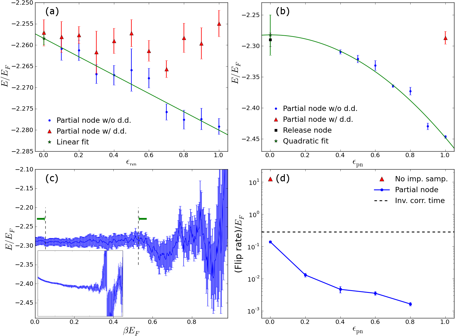
Surprisingly, we find that this algorithm works up to a very high fraction of the original sign violating terms (small ). To obtain the exact answer, we extrapolate to the original Hamiltonian (), heuristically using a quadratic fit (see fig. 3).
To quantify the improvement gained by using the partial node approximation, we measure the average flip rate of the sign of the walkers on the reference determinant (which typically should contain approximately 30% of the walkers for a given snapshot). The flipping of this sign is a signature of an instability of the algorithm coming from the sign problem, and the average flip rate must be significantly below the inverse correlation time for useful data to be garnered from the simulation. Fig. 3d shows the average flip rate using the partial node approximation. Notice that is close to the inverse correlation time, presenting a problem, but by the flip rate has significantly decreased.
V Release Node
In FCI-QMC without annihilation, the sign problem manifests as a variance that scales exponentially with both and the energy difference between the fermionic and bosonic ground states [6]. This exponential scaling in holds even in the presence of annihilation at finite walker number, as annihilation can be thought of as simply reducing the fermion-boson ground state gap. Therefore, minimizing the total needed to reach the ground state wave-function with a certain fidelity also minimizes the effect of the sign problem. Thus, one can improve the convergence time of the importance-sampled FCI-QMC algorithm () by starting very close to the ground state.
One approach to starting near the true ground state is to use the ground state of with a small value of . We aren’t able to explicitly represent this wavefunction, but we can prepare it stochastically via partial node FCI-QMC. The set of walkers thus prepared is then allowed to evolve under the true Hamiltonian for fixed imaginary time . When the wavefunction is “released” to evolve under the exact Hamiltonian, it quickly relaxes to the exact ground state; this is what we call release-node FCI-QMC [14].
In release node, we use the same energy metric as in importance sampled FCI-QMC. In this case, since we have now propagated with two non-commuting Hamiltonians ( and ), one can show that the energy metric only becomes meaningful when the wavefunction reaches the ground state, at which point it gives the ground state energy. As seen in figure 3, the energy converges to the ground state energy before the errors blow up if we start close enough to the ground state. The release node energies agree well with the partial node extrapolation (fig. 3), which provides a check of the validity of our extrapolation.
VI Diagonal dumping
The partial node approximation that we have discussed thus far does not give a variational upper bound on the energy, since we removed the diagonal dumping to get the fixed node Hamiltonian (18). To restore the variational upper bound, we now discuss how one can put the effects of the diagonal dumping back into the partial node algorithm.
While the sum involved in diagonal dumping is in general not analytically tractable, it can be done stochastically in much the same way as off-diagonal spawning. During the diagonal create/kill step [1] we would like to stochastically apply
| (20) |
to a walker on determinant . The first two terms can be done exactly, while the sum – denoted – can be sampled as follows.
- 1.
From pick another determinant according to some normalized probability function .
- 2.
If is not sign-violating, then .
- 3.
Otherwise, .
However, as is now potentially very large, multiplying by weight has the potential to be disastrous if . Therefore, we find it necessary when stochastically dumping the diagonal to also use the approximation
| (21) |
This introduces a time step error which one must extrapolate to zero; empirically a quadratic extrapolation for appears to be quite effective. Partial node results with stochastic dumping of the diagonal are shown in fig. 3.
VII Results
Using partial node FCI-QMC followed by release node, we are able to determine values for the energy and quasiparticle residue of the Fermi-polaron on the BEC side of the interaction, which are shown in fig. 4 for and . The energies are compared to polaron and molecule energies from diagrammatic Monte Carlo [9]. Our results match well for small values of , while for larger values of our energies deviate from the diagrammatic results. This is a consequence of working at fixed , as opposed to diagrammatic Monte Carlo, which is done in the limit . Our results match with the diagrammatic solution after extrapolating to .
Figure 4b shows the quasiparticle residue compared to experimental results [8], where there is a small but finite density of spin-down atoms. We find that, as with the energy, an variational expansion provides a good estimate of . Therefore, as noted elsewhere[8], our theoretical model differs significantly from the experiment, possibly as a result of the finite spin-down density used experimentally.

In extrapolating our results to the physical limit, , we encountered an unexpected problem. Using a linear fit over a wide range of (fig. 4a), we find that individual data points have error well outside the line, with no discernible pattern. Zooming into a very small region of we discovered the reason behind this: small fractional increases in basis size as new shells become available cause large jumps in the ground state energy. A similar issue occurs when attempting to extrapolate in particle number . We nevertheless attempt such an extrapolation in fig. 4 a and b. As a result, the size of the error bars reflects not the accuracy of the data points at individual values of , but rather these inherent shell effects.
Shell effects will vanish in the limit . Therefore, we next address the possibility of extending FCI-QMC into the thermodynamic limit.
VIII FCI-QMC in the thermodynamic limit

All the quantum Monte Carlo simulations described so far have been done for a finite number of particles. In this section, we describe how to modify FCI-QMC to work directly in the thermodynamic limit (TDL, ). In the thermodynamic limit, the accessible momenta span a continuous set of k-points instead of being limited to a discrete grid. Additionally, it is important to work in a representation where instead of enumerating the momenta for all particles, we instead store only their excitations above a known state, in this case . Crucially, in order for the spectrum of the Hamiltonian to remain bounded, allowing application of instead of , the TDL only works with a cutoff on the number of excitations allowed. We note that there are modifications to FCI-QMC that can allow it to work in continuous time, i.e. allow for application of , which we discuss in appendix A. This requirement is similar in spirit to the diagrammatic Monte Carlo method of imposing a cutoff on diagram order, in an attempt to avoid a divergence.
As momentum space is no longer discretized in the TDL, one might assume that annihilation is no longer possible, and therefore that the algorithm is doomed to fail. However, there is one key exception: due to the discrete choice of , annihilation can still occur at that one determinant.
Given this, the TDL algorithm is in practice nearly identical to the algorithm with finite – in fact, one can think of the TDL algorithm as just the limit of the finite algorithm for larger and larger . We have carefully, though implicitly, defined such that all factors of cancel out when determining relevant quantities, such as spawning probability or energy. This is important because taking the limit while at fixed spin-up density (constant ) means taking as well.
The TDL algorithm is remarkably effective at finding the ground state with at unitarity, where the sign problem is weak. These energies at various values of are shown in fig. 5a, where an extrapolation to is much smoother than for finite due to the absence of shell effects.
For the sign-problem-heavy case, we instead show data in the sign-free fixed node limit (), using the diagonal dumping method described in sec. VI. This gives a good energy for the polaron, which is a variational upper bound on the known energy of within error bars. We believe this latter approach of combining fixed node with working directly in the thermodynamic limit will have wide applicability even for the approximate calculations that currently dominate the fermion QMC literature.
IX Discussion
We have shown that the FCI-QMC algorithm can solve the Fermi polaron problem, after improving the algorithm with a smart importance sampled wave function, the introduction of partial and fixed node approximations, and the utilization of release node methods.
We believe that our work demonstrates two main points that should be useful as FCI-QMC and its variants are applied to future problems in condensed matter physics. First, for strongly correlated condensed systems where many determinants are occupied in any single particle basis, we have demonstrated that physical insight – in the form of a good choice of trial wavefunction – can significantly improve the behavior of the FCI-QMC algorithm. Combining the improved statistics of importance sampling with sign-attenuating approximations such as partial node, we showed a significant increase in the effectiveness of FCI-QMC in solving the polaron problem. Finally, we showed that these methods can be made exact, up to statistical noise, via extrapolation or release node QMC.
Second, we have shown that under certain conditions the FCI-QMC algorithm can be extended to work with systems in the thermodynamic limit. Furthermore, we have introduced a fixed node algorithm in this limit, which has historically been an important tool for solving fermionic systems with QMC. We anticipate that these new developments will open a variety of problems in condensed matter physics to be approached using these new developments.
IX.1 Acknowledgments
We would like to thank David Huse and Charles Mathy for valuable discussions. This work was supported in part by ARO Award W911NF-07-1-0464 with funds from the DARPA OLE Program. Some of the computation was performed using the Extreme Science and Engineering Discovery Environment (XSEDE), which is supported by National Science Foundation grant number OCI-1053575. Additional computational work was done on the Feynman cluster at Princeton.
References
- [1] G. H. Booth, A. J. W. Thom, and A. Alavi, Journal of Chemical Physics 131, 054106 (2009).
- [2] D. Cleland, G. H. Booth, and A. Alavi, Journal of Chemical Physics 132, 041103 (2010).
- [3] J. J. Shepherd, G. Booth, A. Grüneis, and A. Alavi, arXiv:1109.2635v1 (2011).
- [4] J. S. Spencer, N. S. Blunt, and W. M. C. Foulkes, arXiv:1110.5479 (2011).
- [5] In practice, one actually applies , where is a tunable parameter that is used to control the number of walkers through a standard feedback process (details can be found in Booth et. al., 2009). This is really a technical point, rather than a physical one, since one could instead apply with occasional resampling.
- [6] M. Kolodrubetz and B. K. Clark, arXiv:1202.0525v1 (2012).
- [7] F. Chevy, Phys. Rev. A 74, 063628 (2006).
- [8] A. Schirotzek, C.-H. Wu, A. Sommer, and M. W. Zwierlein, Phys. Rev. Lett. 102, 230402 (2009).
- [9] N. V. Prokof’ev and B. V. Svistunov, Phys. Rev. B 77, 125101 (2008).
- [10] R. Combescot and S. Giraud, Phys. Rev. Lett. 101, 050404 (2008).
- [11] C. J. M. Mathy, M. M. Parish, and D. A. Huse, Phys. Rev. Lett. 106, 166404 (2011).
- [12] D. M. Ceperley and M. H. Kalos, in Monte Carlo Methods in Statistical Physics, edited by K. Binder (Springer-Verlag, 1979).
- [13] H. J. M. van Bemmel, D. F. B. ten Haaf, W. van Saarloos, J. M. J. van Leeuwen, and G. An, Phys. Rev. Lett. 72, 2442 (1994).
- [14] D. M. Ceperley and B. Adler, Journal of Chemical Physics 81, 5833 (1984).
- [15] S. Sorella and F. Becca, Sissa lecture notes on numerical methods for strongly correlated electrons (2011), URL http://people.sissa.it/~sorella/Simulazioni.pdf.
Appendix A Continuous-time algorithm for FCI-QMC
In this appendix, we introduce a continuous-time FCI-QMC algorithm that has no fixed time step. We note that, while we have not yet implemented this algorithm, the number of off-diagonal terms that must be sampled to remove the penalty method errors (discussed below) is likely to make the algorithm significantly slower than the finite time step algorithms described earlier.
Our continuous-time formulation of FCI-QMC is loosely based on a continuous-time lattice algorithm found elsewhere [15]. We will begin by introducing the algorithm for an arbitrary Hamiltonian , which in general can be some non-Hermitian effective Hamiltonian, as found in importance sampling. We will start by assuming that all off-diagonal sums can be computed analytically, and later generalize this to the case where certain sums must be done stochastically. We generalize the existing algorithm to allow for situations where has a sign problem, so off-diagonal elements of will not be required to be negative.
We would like to apply the propagator , where is now some fixed imaginary time. We refer to as the annihilation time, and think of applying to each walker before performing annihilation. Breaking this up into small time intervals , it becomes . To perform continuous time QMC, we would like to take the limit of this expression.
Consider applying stochastically to some determinant in the limit . We define on-diagonal component and off-diagonal sum , where
| (22) | |||||
We can break up as
| and | (23) |
Then we stochastically apply with probability or with probability .
Furthermore, we would like to choose such that simply corresponds to deterministically moving to with probability proportional to . Thus,
| (24) |
So the algorithm proceeds as follows: start from some determinant , and either apply with probability or with probability . corresponds to hopping to a new determinant. simply multiplies by a weight
| (25) |
is chosen for the first time at step with probability . If , time prior to spawning will come from the probability distribution
| (26) |
Given a choice of from this distribution, the walker will also pick up a total weight during the non-spawning steps, where
| (27) |
Note that, for a non-sign-violating Hamiltonian, the term in the exponent of is just the local energy.
Therefore, for each walker we stochastically propagate for a time , during which it will both hop and pick up weight; this can be done to all the walkers in parallel. Finally, we take all the walkers, perform annihilation, measure observables, and repeat. For Hamiltonians with relatively few off-diagonal terms, i.e. the real-space Hubbard model, this is the complete algorithm. For much larger off-diagonal sums, things become more complicated.
The remainder of this discussion will describe our algorithm for Hamiltonians with large or infinite number of off-diagonal terms in the sums. There are two sums (integrals in the TDL) that we now perform stochastically: the diagonal dumping
| (28) |
and the local potential energy sum
| (29) |
The sums themselves are fairly straightforward. Using the same method as spawning in FCI-QMC, we have a method for generating determinant connected by an off-diagonal component of to the starting determinant . If the probability to generate is , then for example is just the expectation of the observable
| (30) |
A similar observable can be defined for computing . Assume that we have sampled a total of determinants to simultaneously calculate and with some mean and standard error for each observable.
Formally, we could perform this sampling in the limit , determine and exactly, and simply use them in the earlier procedure. However, for finite , we want to utilize a variant of the penalty method to minimize the bias due to statistical uncertainty. Consider first the simpler case of applying the weight . Assume that the actual value of is drawn from a Gaussian distribution with mean and width , which are given by the expectation value and standard error of . Then the weight we should apply is simply
| (31) |
A more complicated question is how to sample in an unbiased way. Again, assume that is drawn from a Gaussian . Furthermore, assume that we have chosen large enough that we don’t have to worry about the negative tail of the Gaussian, i.e. . We want to sample from the full distribution
| (32) |
We can expand to second order in , ignoring the first order term (whose integral vanishes). Then
| (33) | |||||
| (34) |
Normalizing and integrating this result, we find that the normalized cumulative distribution function is
| (35) |
We can then sample from this distribution by picking at random, then finding the value of where .
In summary, here is our algorithm for continuous partial node FCI-QMC:
- 1.
Start with walkers, each with weight , sign , and determinant . At the first step, all walkers are initialized in with positive sign. At this point, there should be no walkers with the same determinant but opposite sign.
- 2.
Propagate each walker independently by as follows. At the start of this portion, define a variable for each walker, and initialize .
- (a)
For a walker in determinant , sample off-diagonal elements for steps to get , , , and .
- (b)
Sample from as described above, where and .
- (c)
If , then move the walker to a new determinant . To sample with weight proportional to , run a Metropolis algorithm for steps. The sign of is (not) flipped when the matrix element is positive (negative).
- (d)
Multiply the weight by , with the stochastic portion of re-weighted via the penalty method as described above. If , then use in place of in these formulas.
- (e)
Increment by . If , repeat from part (a).
- (a)
- 3.
Annihilate the walkers, keeping track of their weights. For example, if five walkers are all on determinant with weights to and signs to , let . Then the five walkers are replaced by a single walker with weight and sign .
- 4.
Resample the walkers. Replace a single walker with weight by walkers of weight 1. Add another walker of weight 1 with probability .
- 5.
Measure observables.
- 6.
Adjust using standard feedback protocols [1] as desired. Then repeat from step 1.