Stochastic finite differences and multilevel Monte Carlo for a class of SPDEs in finance

Integrating (2) over the time interval $[t,t\!+\!k]$ gives

$$v(t\!+\!k,x)=v(t,x)+\int_{t}^{t+k}\left(-\,\mu\frac{\partial v}{\partial x}+\frac{1}{2}\,\frac{\partial^{2}v}{\partial x^{2}}\right)\,{\rm d}s-\int_{t}^{t+k}\!\!\sqrt{\rho}\ \frac{\partial v}{\partial x}\,\,{\rm d}M_{s}.$$

Making the approximation $v(s,x)\!\approx\!v(t,x)$ for $t\!<\!s\!<\!t\!+\!k$ in the first integral and

$$v(s,x)\approx v(t,x)-\sqrt{\rho}\left.\frac{\partial v}{\partial x}\right|_{(t,x)}(M_{s}\!-\!M_{t})$$

in the second, and noting the standard Itô calculus result that

$$\int_{t}^{t+k}(M_{s}\!-\!M_{t})\,\,{\rm d}M_{s}=\frac{1}{2}\left(\rule{0.0pt}{11.56346pt}(\Delta M^{n})^{2}\!-\!k\right),$$

where $\Delta M^{n}\equiv M_{t+k}-M_{t}=\sqrt{k}\,Z_{n}$ with $Z_{n}\sim N(0,1)$, [Glasserman(2004), Kloeden & Platen(1992)], leads to the Milstein semi-discrete approximation

$$v^{n+1}(x)=v^{n}(x)-(\mu\,k+\sqrt{\rho\,k}\,Z_{n})\,\frac{\partial v^{n}}{\partial x}+\frac{1}{2}\left(\rule{0.0pt}{11.56346pt}(1\!-\!\rho)\,k+\rho\,k\,Z_{n}^{2}\right)\frac{\partial^{2}v^{n}}{\partial x^{2}}.$$

Using a spatial grid with uniform spacing $h$, standard central difference approximations to the spatial derivatives [Richtmyer & Morton(1967)] then give the finite difference equation

	$\displaystyle v_{j}^{n+1}$	$\displaystyle=$	$\displaystyle v_{j}^{n}\ -\ \frac{\mu\,k+\sqrt{\rho\,k}\,Z_{n}}{2h}\left(v_{j+1}^{n}-v_{j-1}^{n}\right)$		(10)
			$\displaystyle~~~~+\ \frac{(1\!-\!\rho)\,k+\rho\,k\,Z_{n}^{2}}{2h^{2}}\left(v_{j+1}^{n}-2v_{j}^{n}+v_{j-1}^{n}\right),$

in which $v_{j}^{n}$ is an approximation to $v(nk,jh)$.

The spatial domain is truncated by introducing an upper boundary at $x_{max}\!=\!J\,h$ and using the boundary condition $v_{J}^{n}\!=\!0$. Since the initial distribution will be assumed localised, both the localisation error for a given path $M$, and the expected error of functionals of the solution, can be made as small as needed by a large enough choice $x_{max}>0$.

The system of SDEs can then be written in matrix-vector form

$\displaystyle V_{n+1}$

$\displaystyle=$

$\displaystyle V_{n}\ -\ \frac{\mu\,k+\sqrt{\rho\,k}\,Z_{n}}{2h}D_{1}V_{n}+\ \frac{(1\!-\!\rho)\,k+\rho\,k\,Z_{n}^{2}}{2h^{2}}D_{2}V_{n},$

(11)

where $V_{n}$ is the vector with elements $v_{j}^{n},j=1,\ldots,J\!-\!1$ and $D_{1}$ and $D_{2}$ are the matrices corresponding to first and second central differences as explicitly given in Appendix A.

To approximate the initial condition on the grid, we apply the initial measure $\nu^{N}_{0}$ to a basis of ‘hat functions’ $\left\langle\Psi_{j}\right\rangle_{0<j<J}$, where

$$\Psi_{j}(x)=\frac{1}{h}\max\left(h-|x-x_{j}|,0\right),$$

giving

$$v_{j}^{0}=\langle\Psi_{j},v_{0}\rangle=\int_{-\infty}^{\infty}\Psi_{j}(x)\ v_{0}(x){\,\rm d}x.$$

For the corresponding PDE ($\rho=0$), this is known to result in $O(h^{2})$ convergence provided $k$ satisfies a certain stability limit, even when the initial data are not smooth [Pooley et al.(2003), Carter & Giles(2007)]. We will see that an extension of this analysis holds for SPDEs.

Finite difference Fourier stability analysis ignores the boundary conditions and considers Fourier modes of the form

$$v_{j}^{n}=g_{n}\exp(ij\theta),\quad|\theta|\leq\pi,$$

(13)

which satisfy (10) provided

$$g_{n+1}=\left(a(\theta)+b(\theta)\,Z_{n}+c(\theta)\,Z_{n}^{2}\right)g_{n},$$

where

	$\displaystyle a(\theta)$	$\displaystyle=$	$\displaystyle 1-\frac{i\,\mu\,k}{h}\,\sin\theta-\frac{2\,(1\!-\!\rho)\,k}{h^{2}}\sin^{2}{\textstyle\frac{\theta}{2}},$
	$\displaystyle b(\theta)$	$\displaystyle=$	$\displaystyle-\,\frac{i\sqrt{\rho\,k}}{h}\,\sin\theta,$
	$\displaystyle c(\theta)$	$\displaystyle=$	$\displaystyle-\,\frac{2\,\rho\,k}{h^{2}}\sin^{2}{\textstyle\frac{\theta}{2}}.$

Following the approach of mean-square stability analysis from [Higham(2000), Saito & Mitsui(1996)], we obtain

	$\displaystyle\mathbb{E}[\,|g_{n+1}|^{2}]$	$\displaystyle=$	$\displaystyle\mathbb{E}\left[(a+b\,Z_{n}+c\,Z_{n}^{2})(a^{*}+b^{*}Z_{n}+c^{*}Z_{n}^{2})\ |g_{n}|^{2}\right]$
		$\displaystyle=$	$\displaystyle\left(\,|a\!+\!c|^{2}+|b|^{2}+2|c|^{2}\,\right)\ \mathbb{E}\left[\,|g_{n}|^{2}\right],$

where $a^{*}$ denotes the complex conjugate of $a$. Mean-square stability therefore requires

	$\displaystyle|a|^{2}+|b|^{2}+3|c|^{2}+a\,c^{*}+a^{*}c$
	$\displaystyle=\ 1-4\sin^{2}{\textstyle\frac{\theta}{2}}\left\{\frac{k}{h^{2}}-(1+2\rho^{2})\left(\frac{k}{h^{2}}\right)^{2}\sin^{2}{\textstyle\frac{\theta}{2}}-\left(\left(\frac{\mu\,k}{h}\right)^{2}+\frac{\rho\,k}{h^{2}}\right)\cos^{2}{\textstyle\frac{\theta}{2}}\right\}$
	$\displaystyle\leq\ 1,$

and enforcing this for all $\theta$ leads to the two conditions summarised in the following theorem.

The analysis in Appendix A combines mean-square and matrix stability analysis to prove that in the limit $k,h\rightarrow 0$ the condition $k/h^{2}\leq(1+2\rho^{2})^{-1}$ is also a sufficient condition for mean-square stability of the initial-boundary value problem with the boundary conditions at $j\!=\!0$ and $j\!=\!J$.

Fourier analysis can also be used to examine the accuracy of the finite difference approximation in the absence of boundary conditions. Considering a Fourier mode of the form $g(t)\exp(i\kappa x),$ the PDE (4) reveals that

$$g(t)=g(0)\ \exp\left(\rule{0.0pt}{11.56346pt}\!-{\textstyle\frac{1}{2}}(1\!-\!\rho)\,\kappa^{2}\,t-i\,\kappa\,(\mu\,t+\sqrt{\rho}\,M_{t})\right),$$

and therefore

$$g(t_{n+1})=g(t_{n})\ \exp\left(\rule{0.0pt}{11.56346pt}\!-{\textstyle\frac{1}{2}}(1\!-\!\rho)\,\kappa^{2}\,k-i\,\kappa\,(\mu\,k\!+\!\sqrt{\rho\,k}\,Z_{n})\right),$$

where $M_{t_{n+1}}-M_{t_{n}}=\sqrt{k}\,Z_{n}$. Fourier analysis of the discretisation gives

$$g_{n+1}=\left(a(\kappa h)+b(\kappa h)\,Z_{n}+c(\kappa h)\,Z_{n}^{2}\right)g_{n},$$

where $a(\theta)$, $b(\theta)$, $c(\theta)$ are as defined before. Writing

$$a(\kappa h)+b(\kappa h)\,Z_{n}+c(\kappa h)\,Z_{n}^{2}=\exp\left(\rule{0.0pt}{11.56346pt}\!-{\textstyle\frac{1}{2}}(1\!-\!\rho)\,\kappa^{2}\,t-i\,\kappa\,(\mu\,k\!+\!\sqrt{\rho\,k}\,Z_{n})+e_{n}\right)$$

we obtain, after performing lengthy expansions using MATLAB’s Symbolic Toolbox,

$$e_{n}=\sqrt{\rho\,k}\ \kappa^{2}\mu\,k\,Z_{n}-{\textstyle\frac{1}{6}}i\,\sqrt{\rho\,k}\ \kappa^{3}Z_{n}\left(\rule{0.0pt}{11.56346pt}3\,(1\!-\!\rho)\,k+\rho\,k\,Z_{n}^{2}-h^{2}\right)+r_{n},$$

where, for all $p\geq 1$,

$$\mathbb{E}[|r_{n}|^{p}]\leq c(\kappa,p)\left(k^{2}+kh^{2}\right)^{p}.$$

When summing over $T/k$ timesteps, $\sum Z_{n}$ and $\sum Z^{3}_{n}$ are both $O(k^{-1/2})$ since they have zero expectation and $O(k^{-1})$ variance. Hence, it follows that

$$\left(\mathbb{E}\left[\left(\sum_{n}e_{n}\right)^{2}\right]\right)^{1/2}=O(k,h^{2}),$$

so the RMS error in the Fourier mode over the full simulation interval is $O(k,h^{2})$.

Following the method of analysis in [Carter & Giles(2007)], it can be deduced from this that the RMS $L_{2}$ and $L_{\infty}$ errors for $V_{n}$ are both $O(k,h^{2})$. This is consistent with the usual $O(k,h^{2})$ accuracy of the forward-time central space discretisation of a parabolic PDE [Richtmyer & Morton(1967)], and the $O(k)$ strong accuracy of the Milstein discretisation of an SDE, see e.g. [Kloeden & Platen(1992)].

We now test the accuracy and stability of the scheme numerically.

The chosen parameters for (2) are $\sigma=0.22$, $\rho=0.2$, $r=0.042$, $\mu=(r-\sigma^{2}/2)/\sigma$, $v(0,x)\!=\!\delta(x\!-\!x_{0})$ with $x_{0}=5$. These values are typical for the applications later on.

The upper boundary for the computation is $x_{max}=16$, and chosen to ensure that the use of zero Dirichlet data has negligible influence on the solution.

We approximate the initial value problem without boundary conditions on $[-16/3,16]$ (note $x_{0}=5$ is roughly in the centre), and also the initial-boundary value problem with zero Dirichlet conditions on $[0,16]$.

Figure 1 plots several solutions to the latter problem at $T=5$, each corresponding to a different Brownian path $M_{t}$.

It can be seen that for those realisations for which $M_{t}$ has been largely positive, the boundary at $x\!=\!0$ has had negligible influence and so the solution is approximately equal to the displaced Normal distribution given by (6).

For the unbounded case, we approximate the mean-square $L_{2}$-error by

	$\displaystyle E(h,k)^{2}$	$\displaystyle=$	$\displaystyle\mathbb{E}\left[\sum_{j=0}^{J}(v_{j}^{N}(\omega)-v(Nk,jh;\omega))^{2}\,h\right]$		(16)
		$\displaystyle\approx$	$\displaystyle\frac{1}{M}\sum_{m=1}^{M}\sum_{j=0}^{J}(v_{j}^{N}(\omega_{m})-v(Nk,jh;\omega_{m}))^{2}\,h,$

where $J$ is the number of grid intervals, $N$ the number of timesteps, and the expectation is taken over Brownian paths $\omega$, of which $\omega_{m}$ are $M$ samples.

To study the convergence, we introduce decreasing grid sizes $h_{l}=h_{0}\,2^{-l}$ and timesteps $k_{l}=k_{0}\,4^{-l}$, motivated by the second order convergence in $h$ and first order convergence in $k$ as well as the stability limit for the explicit scheme, and denote $E_{l}=E(h_{l},k_{l})$ the mean-square $L_{2}$-error at level $l$.

For the initial-boundary value problem, no analytical solution is known, but we can compute error indicators via the difference between a fine grid solution $f$ with mesh parameters $k$ and $h$, and a coarse solution $c$ with mesh parameters $4k$ and $2h$,

	$\displaystyle e(h,k)^{2}$	$\displaystyle=$	$\displaystyle\mathbb{E}\left[\sum_{j=0}^{J/2}(f_{2j}^{N}(\omega)-c_{j}^{N/4}(\omega))^{2}\,h\right]$		(17)
		$\displaystyle\approx$	$\displaystyle\frac{1}{M}\sum_{m=1}^{M}\sum_{j=0}^{J/2}(f_{2j}^{N}(\omega_{m})-c_{j}^{N/4}(\omega_{m}))^{2}\,h,$

and define $e_{l}=e(h_{l},k_{l})$.

On the coarsest level, $h_{0}=4/3$, $k_{0}=1/4$, such that $x_{0}$ does not coincide with a grid point.

Fig. 2 shows both the computed values of $E_{l}^{2}$ and $e_{l}^{2}$ for the unbounded case, and $e_{l}^{2}$ for the bounded case.

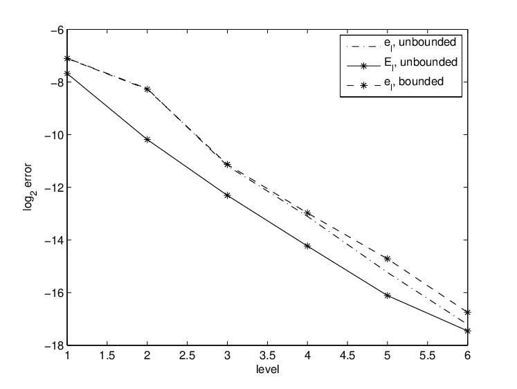
The results confirm the theoretical $O(k,h^{2})$ convergence in the unbounded case, and support the conjecture that the convergence order is unchanged in the bounded case.

We now formalise this conjecture about the error due to the SPDE discretisation. Denote $U_{T}=u(T,\cdot)$ the solution to the initial boundary value problem at time $T$ for a given Brownian path and $\widehat{U}_{T}$ its numerical approximation with grid size $h$ and timestep $k\propto h^{2}$.

We know Conjecture 2.1 to be true for the initial value problem on $\mathbb{R}$, and it conjectures that the introduction of the boundary condition at $x\!=\!0$ does not affect the (weak and) strong error, which is supported by the numerical results.

The conjecture assumes $x_{max}\!=\!\infty$; in practice, a finite value for $x_{max}$ will introduce an additional truncation error which will decay exponentially in $x_{max}$.

Numerical tests with different parameters, not reproduced here, indicate that the error in the bounded case increases for values of $x_{0}$ close to 0, in which case more paths contribute solutions with large higher derivatives close to the zero boundary, even if the asymptotic convergence order is still $O(k,h^{2})$. We analyse this loss of regularity further in Appendix B.

Basket credit derivatives provide protection against the default of a certain segment (‘tranche’) of a basket of firms. A typical example is that of a collateralized debt obligation where the protection buyer receives a notional amount, minus some recovery proportion $0\leq R\leq 1$, if firms in a specified tranche of the basket default, and in return pays a regular spread until the default event occurs.

The arbitrage-free spread depends crucially on the (risk-neutral, when hedged with defaultable bonds) probability of joint defaults. For a tranche with attachment point $0\leq a<1$ and detachment point $1\geq d>a$, the outstanding tranche notional

$$P(L_{t})=\max(d-L_{t},0)-\max(a-L_{t},0),$$

(20)

where the loss variable $L_{t}$ is the proportion of losses in the basket up to time $t$, determines the spread and default payments related to that tranche. The risk-neutral value of the tranche spread can be derived as

$$s=\frac{\sum_{i=1}^{n}\,{\rm e}^{-rT_{i}}\mathbb{E}^{\mathbb{Q}}[P(L_{T_{i-1}})-P(L_{T_{i}})]}{\delta\sum_{i=1}^{n}\,{\rm e}^{-rT_{i}}\mathbb{E}^{\mathbb{Q}}[P(L_{T_{i}})]},$$

(21)

see, e.g., [Bush et al.(2011)]. Here, $n$ is the maximum number of spread payments, $T$ the expiry, $T_{i}$ the payment dates for $1\leq i\leq n$, $\delta=0.25$ the interval between payments. Spreads are quoted as an annual payment, as a ratio of the notional, but assumed to be paid quarterly. ¹¹ 1 There is a variation for the equity tranche, and recently sometimes the mezzanine tranche, but we do not go into details here.

For an extensive survey of credit derivatives and pricing models we refer the reader to [Schönbucher(2003)], and note only that they typically fall in one of two classes: so-called reduced-form models, which model default times of firms directly as (dependent) random variables; structural models, which capture the evolution of the firms’ values, and model default events as the first passage of a lower default barrier. We will consider the latter here.

In a structural model in the spirit of the classical works of [Merton(1974)] and [Black & Cox(1976)], as extended to multiple firms e.g. in the work of [Hull et al.(2005)], a company $i$’s firm value, $1\leq i\leq N$, is assumed to follow a model of the type

$$\frac{\,{\rm d}A_{t}^{i}}{A_{t}^{i}}=r\,{\rm d}t+\sqrt{1\!-\!\rho_{i}}\ \sigma_{i}\,{\rm d}W_{t}^{i}+\sqrt{\rho_{i}}\ \sigma_{i}\,{\rm d}M_{t},\qquad A_{0}^{i}=a^{i},$$

where $0\leq\rho_{i}\leq 1$ is a correlation parameter, $r$ is the risk-free interest rate, $\sigma_{i}$ the volatility, and $M$, $W^{i}$ are standard Brownian motions.

Here, the individual firms are correlated through a common ‘market’ factor $M$, but independent conditionally on $M$. We make in the following the assumption that the firms are exchangeable in the sense that their dynamics is governed by the same set of parameters, specifically $\rho=\rho_{i}$, $\sigma=\sigma_{i}$. Their initial values $a_{i}$ are not necessarily identical which allows for different default probabilities for individual firms, consistent with their CDS spreads.

In this framework, the default time $T_{0}^{i}$ of the $i$-th firm is modelled as the first hitting time of a default barrier $B^{i}$, for simplicity constant, and the distance-to-default

$$X_{t}^{i}=\frac{1}{\sigma}\left(\,\log A_{t}^{i}-\log B^{i}\,\right),$$

(22)

evolves according to (3), where $\mu=\left(r-\frac{1}{2}\sigma^{2}\right)/\sigma$, $x^{i}=\left(\,\log a^{i}-\log B^{i}\,\right)/\sigma$. $T^{i}_{0}$ as in (7) is precisely the default time.

In the majority of applications, Monte Carlo simulation of the firm value processes is used for the estimation of tranche spreads, see e.g. [Hull et al.(2005)] or [Fouque et al.(2008), Carmona et al.(2009)]. This is largely enforced by the size of $N$, for instance in the case of index tranches $N=125$.

This, however, puts the model precisely in the realm of the large basket approximation (2). See [Bujok & Reisinger(2012)] for a numerical study of this large basket approximation. The loss functional is thereby approximated by

$$\widehat{L}_{T_{i}}=(1-R)\left(1-h\sum_{j=1}^{J-1}v_{j}^{T_{i}/k}\right)$$

in terms of the numerical SPDE solution $v_{j}^{T_{i}/k}$ at time $T_{i}$, which feeds into the estimator for the outstanding tranche notional (20) and subsequently the tranche spreads (21).

All following results are for a representative set of parameter values, taken from a calibration performed in [Bush et al.(2011)] to 2007 market data, $\sigma=0.22$, $\rho=0.2$, $r=0.042$, $\mu=(r-\sigma^{2}/2)/\sigma$. While the initial distribution used in [Bush et al.(2011)] is somewhat spread out to match individual CDS spreads of obligors, most of the mass is around $x_{0}=5$ and for simplicity we centre all firms there for the numerical tests, $v(0,x)\!=\!\delta(x\!-\!x_{0})$. The upper boundary is chosen as $x_{max}=16$.

We consider a maturity $T=5$ and tranches $[a,d]=[0,0.03]$, $[0.03,0.06]$, $[0.06,0.09]$, $[0.09,0.12]$, $[0.12,0.22]$, $[0.22,1]$.

Figure 3 shows the multilevel results for the expected protection payment from the first tranche,

$$\sum_{i=1}^{n}\,{\rm e}^{-rT_{i}}\mathbb{E}^{\mathbb{Q}}[P(\widehat{L}_{T_{i-1}})-P(\widehat{L}_{T_{i}})],$$

expressed as a fraction of the initial tranche notional.

We pick mesh sizes $h_{l}=h_{0}\,2^{-l}$ and $k_{l}=k_{0}\,4^{-l}$ for $l>0$ and $h_{0}=8/5$, $k_{0}=1/4$. This is motivated by the second and first order consistency in $h$ and $k$ respectively, and within the stability limit (15).

The top-left plot shows the convergence of the variance $\mathbb{V}[\widehat{P}_{l}\!-\!\widehat{P}_{l-1}]$ as well as the variance of the standard single level estimate, while the top-right plot shows the convergence of the expectation $\mathbb{E}[\widehat{P}_{l}\!-\!\widehat{P}_{l-1}]$.

The bottom-left plot shows results for different multilevel calculations, each with a different user-specified accuracy requirement. For each value of the accuracy $\varepsilon$, the multilevel algorithm determines (by formula (12) from [Giles(2008a)]) the numbers of levels of refinement which are needed to ensure that the contribution to the Mean Square Error (MSE) due to the weak error on the finest grid is less than ${\textstyle\frac{1}{2}}\varepsilon^{2}$, and it determines (by formula (10) from [Giles(2008a)]) the optimal number of samples on each level so that the combined variance of the multilevel estimate is also less than ${\textstyle\frac{1}{2}}\varepsilon^{2}$, and hence the MSE is less than $\varepsilon^{2}$.

Treating a single finite difference calculation on the coarsest level as having a unit cost, the bottom-right plot compares the total cost of the standard and multilevel algorithms. Since the objective is to achieve a computational cost which is approximately proportional to $\varepsilon^{-2}$, it is the cost $C$ multiplied by $\varepsilon^{2}$ which is plotted versus $\varepsilon$. The results confirm that $\varepsilon^{2}C$ does not vary much as $\varepsilon\rightarrow 0$ for the multilevel method, in line with the prediction that $\varepsilon^{2}C\propto 1$, whereas it grows significantly for the standard method since $\varepsilon^{2}C\propto 8^{L}$, where $L$ is the index of the finest level. Hence, there is a big jump in the cost of the standard method each time it is necessary to switch to a finer level to ensure the weak error is less than $\varepsilon/\sqrt{2}$, whereas the jump is minimal for the multilevel method.

In practice, default is not monitored continuously but only at a discrete set of times, and for pricing often the simplifying assumption is made that default is only determined at the spread payment dates $T_{l}$.

This can be incorporated as follows. In the time intervals $(T_{l-1},T_{l})$, we solve (2) on a sufficiently large domain (e.g. $[-4,16]$), and apply the following interface conditions at $T_{l}$:

$$\lim_{t\downarrow T_{l}}v(t,x)=\left\{\begin{array}[]{rl}0,&x\leq 0,\\ \lim_{t\uparrow T_{l}}v(t,x),&x>0.\end{array}\right.$$

(23)

To maintain quadratic grid convergence in spite of the discontinuity introduced by (23), we choose the mesh such that a grid point coincides with the 0 boundary (e.g. by setting $h_{0}=2$ in the above example), and set the numerical solution after default monitoring to 0 for grid coordinates below 0 and to $1/2$ its previous value at 0, see e.g. [Pooley et al.(2003)].

It is seen in Fig. 4 that convergence is very similar to the previous case.

Here we discuss the computational complexity of the multilevel solution of the SPDE compared with the alternative use of the multilevel method for solving the SDEs which arise from directly simulating a large number of SDEs.

We have already explained that to achieve a r.m.s. accuracy of $\varepsilon$ requires $O(\varepsilon^{-7/2})$ work when solving the SPDE by the standard Monte Carlo method, but the cost is $O(\varepsilon^{-2})$ using the multilevel method, provided Conjecture 2.1 is correct.

Consider now the alternative of using a finite number of particles (firms), $M$, to estimate the tranche loss in the limit of an infinite number of particles (firms). In this case, empirical results suggest that there is an additional $O(M^{-1})$ error (see also [Bujok & Reisinger(2012)]), and the proof of this convergence order is the subject of current research. Taking this to be the case, the optimal choice of $M$ to minimise the computational complexity to achieve an r.m.s. error of $\varepsilon$ is $O(\varepsilon^{-1})$. Using the standard Monte Carlo method, the optimal timestep is $O(\varepsilon)$, and the optimal number of paths is $O(\varepsilon^{-2})$, so the overall cost is $O(\varepsilon^{-4})$. Using the multilevel method for the SDEs reduces the cost per company to $O(\varepsilon^{-2})$, so the total cost is $O(\varepsilon^{-3})$.

This complexity information is summarised in Table 1. There is also a practical implementation aspect to note. The computational cost per grid point in the finite difference approximation of the SPDE is minimal, requiring just three floating point multiply-add operations if equation (10) is re-cast as

$$v_{j}^{n+1}=av_{j-1}^{n}+bv_{j}^{n}+cv_{j+1}^{n}$$

with the coefficients $a,b,c$ computed once per timestep, for all $j$.

References

- [Bain & Crisan(2009)] Bain, A. & Crisan, D. Fundamentals of Stochastic Filtering, Springer, 2009.
- [Barth et al.(2010)] Barth, A., Schwab, C., & Zollinger, N. Multi-level Monte Carlo finite element method for elliptic PDEs with stochastic coefficients, Num. Math., 119(1):123-161, 2010.
- [Benth & Koekebakker(2008)] Benth, F.E. & Koekebakker, S. Stochastic modeling of financial electricity contracts, Energy Economics, 30(3):1116–1157, 2008.
- [Black & Cox(1976)] Black, F. and Cox, J. Valuing corporate securities: some effects of bond indenture provision, J. Finance, 31:351–367, 1976.
- [Bruti-Liberati & Platen(2010)] Bruti-Liberati, N. & Platen, E. Numerical Solution of Stochastic Differential Equations with Jumps in Finance, Springer, 2010.
- [Buckwar & Sickenberger(2011)] Buckwar, E. & Sickenberger, T. A comparative linear mean-square stability analysis of Maruyama- and Milstein-type methods, Math. Comp. Sim., 81:1110–1127, 2011.
- [Bujok & Reisinger(2012)] Bujok, K. & Reisinger, C. Numerical Valuation of Basket Credit Derivatives in Structural Jump-Diffusion Models, J. Comp. Fin., to appear.
- [Bush et al.(2011)] Bush, N., Hambly, B., Haworth, H., Jin, L., & Reisinger, C. Stochastic evolution equations in portfolio credit modelling, SIAM Fin. Math., 2(1):627–664, 2011.
- [Carmona et al.(2009)] Carmona, R., Fouque, J.-P., & Vestal, D, Interacting particle systems for the computation of rare credit portfolio losses, Fin. Stoch., 13(4):613–633, 2009.
- [Carter & Giles(2007)] Carter, R. & Giles, M.B. Sharp error estimates for discretisations of the 1D convection/diffusion equation with Dirac initial data, IMA J. Num. Anal., 27(2):406–425, 2007.
- [Cliffe et al.(2011)] Cliffe, K.A., Giles, M.B., Scheichl, R., & Teckentrup, A.L. Multilevel Monte Carlo methods and applications to elliptic PDEs with random coefficients, Computing and Visualization in Science, 14(1):3–15, 2011.
- [Fouque et al.(2008)] Fouque, J., Wignall B., & Zhou, X. Modeling correlated defaults: first passage model under stochastic volatility. J. Comp. Fin., 11(3): 43–78, 2008.
- [Giles(2008a)] Giles, M.B. Multi-level Monte Carlo path simulation, Operations Research, 56(3):981–986, 2008.
- [Giles(2008b)] Giles, M.B. Improved multilevel Monte Carlo convergence using the Milstein scheme, pp. 343–358 in Monte Carlo and Quasi-Monte Carlo Methods 2006, editors Keller, A., Heinrich, S., & Niederreiter, H., Springer-Verlag, 2008.
- [Glasserman(2004)] Glasserman, P. Monte Carlo Methods in Financial Engineering, Springer, 2004.
- [Graubner(2008)] Graubner, S. Multi-level Monte Carlo Methoden für stochastische partielle Differentialgleichungen. Diplomarbeit, TU Darmstadt, 2008.
- [Gyöngy(1999)] Gyöngy, I. Lattice approximations for stochastic quasi-linear parabolic partial differential equations driven by space-time white noise II, Potential Anal., 11:1–37, 1999.
- [Gyöngy & Nualart(1997)] Gyöngy, I. & Nualart, D. Implicit schemes for stochastic quasi-linear parabolic partial differential equations driven by space-time white noise, Potential Anal., 7:725–757, 1997.
- [Heath et al.(1992)] Heath, D., Jarrow, R., & Morton, A. Bond pricing and the term structure of interest rates: A new methodology for contingent claims valuation, Econometrica, 60(1):77–105, 1992.
- [Higham(2000)] Higham, D.J. Mean-square and asymptotic stability of the stochastic theta method, SIAM J. Num. Anal., 38(3):753–769, 2000.
- [Hull et al.(2005)] Hull, J., Predescu, M., & White, A. The valuation of correlation-dependent credit derivatives using a structural model, J. Credit Risk, 6(3):99–132, 2005.
- [Kloeden & Platen(1992)] Kloeden, P.E. & Platen, E. Numerical Solution of Stochastic Differential Equations, Springer, 1992.
- [Krylov(1994)] Krylov, N.V. A -theory of the Dirichlet problem for SPDEs in general smooth domains, Probab. Theory Relat. Fields, 98:389–421, 1994.
- [Kurtz & Xiong(1999)] Kurtz, T.G. & Xiong, J. Particle representations for a class of nonlinear SPDEs, Stoch. Proc. Appl., 83:103–126, 1999.
- [Lang(2010)] Lang, A. A Lax equivalence theorem for stochastic differential equations, J. Comp. Appl. Math., 234(12):3387–3396, 2010.
- [Merton(1974)] Merton, R., On the pricing of corporate debt: The risk structure of interest rates, J. Fin., 29:449–470, 1974.
- [Pooley et al.(2003)] Pooley, D.M., Vetzal, K.R., & Forsyth, P.A. Remedies for non-smooth payoffs in option pricing, J. Comp. Fin., 6:25–40, 2003.
- [Richtmyer & Morton(1967)] Richtmyer, R.D. & Morton, K.W. Difference Methods for Initial-Value Problems, Wiley-Interscience, 1967.
- [Roth(2002)] Roth, C. Difference methods for stochastic partial differential equations, Z. Angew. Math. Mech., 82(11–12):821–830, 2002.
- [Roth(2006)] Roth, C. A combination of finite difference and Wong-Zakai methods for hyperbolic stochastic partial differential equations, Stoch. Anal. Appl., 24(1):221–240, 2006.
- [Saito & Mitsui(1996)] Saito, Y. & Mitsui, T. Stability analysis of numerical schemes for stochastic differential equations, SIAM J. Num. Anal., 33(6):2254–2267, 1996.
- [Schönbucher(2003)] Schönbucher, P.J. Credit Derivatives Pricing Models, Wiley, 2003.
- [Walsh(2005)] Walsh, J.B. Finite element methods for parabolic stochastic PDEs, Potential Anal., 23:1–43, 2005.
- [Xia & Giles(2012)] Xia, Y. & Giles, M.B. Multilevel path simulation for jump-diffusion SDEs, in Monte Carlo and Quasi-Monte Carlo Methods 2010, editors Wozniakowski, H. & Plaskota, L., Springer-Verlag, 2012.
- [Zhou(2001)] Zhou, C., An analysis of default correlations and multiple defaults, The Review of Financial Studies, 14:555–576, 2001.
Appendix A Mean-square matrix stability analysis
If is the vector with elements then the finite difference equation can be expressed as
where is the identity matrix and and are the matrices corresponding to central first and second differences, which for are
From the recurrence relation we get
Noting that is anti-symmetric and is symmetric, and that
where corresponds to a central second difference with twice the usual span,
(with the end values of being chosen to correspond to and ), and and are each entirely zero apart from one corner element,
then after some lengthy algebra we get
where
and
It can be verified that the eigenvector of has elements for , and the associated eigenvalue is
where are the same functions as defined in the mean-square Fourier analysis. In addition, in the limit , , and therefore in this limit the Fourier stability condition
is also a sufficient condition for mean-square matrix stability.
Appendix B Regularity considerations
Figure 5 shows the convergence behaviour as the computational grid is refined. Level 0 has ; is reduced by factor 2 and by factor in moving to finer levels.
The top-left plot shows the convergence of , with notation as in Sections 3 and 4.2; the top-right plot shows the convergence of .
The bottom two plots show the behaviour of , which is estimated on each grid level using the standard second difference
The left plot indicates that the mean of this quantity is well behaved, but the right plot indicates a singular behaviour of its variance, with the value increasing rapidly with increased grid resolution.
This is in accordance with the result shown in [Krylov(1994)], that for the unique solution to the SPDE, is square integrable, but has a singularity at 0.