Study of $B_{c}\rightarrow D_{s}^{*}\,\ell^{+}\ell^{-}$ in Single Universal Extra Dimension

Flavor-changing neutral current (FCNC) $b\rightarrow s,d$ transitions which occur at loop level in the standard model (SM) provide us a powerful tool to test the SM and also a frame to study physics beyond the SM. After the observation of $b\rightarrow s\,\gamma$ [1], these transitions became more attractive and since then rare radiative, leptonic and semileptonic decays of $B_{u,d,s}$ mesons have been intensively studied [2]. Among these decays, semileptonic decay channels are significant because of having relatively larger branching ratio. The experimental data for exclusive $B\rightarrow K^{(*)}\ell^{+}\ell^{-}$ also increased the interest in these decays. These studies will be even more complete if similar studies for $B_{c}$, discovered by CDF Collaboration [3], are also included.

The $B_{c}$ meson is the lowest bound state of two heavy quarks, bottom $b$ and charm $c$, with explicit flavor that can be compared with the $c\bar{c}$ and $b\bar{b}$- bound state which have implicit flavor. The implicit-flavor states decay strongly and electromagnetically whereas the $B_{c}$ meson decays weakly. $B_{u,d,s}$ are described very well in the framework of the heavy quark limit, which gives some relations between the form factors of the physical process. In case of $B_{c}$ meson, the heavy flavor and spin symmetries must be reconsidered because of heavy $b$ and $c$. On the experimental side of the decay, for example, at LHC, $10^{10}B_{c}$ events per year is estimated [4]-[5]. This reasonable number is stimulating the work on the $B_{c}$ phenomenology and this possibility will provide information on rare $B_{c}$ decays as well as CP violation and polarization asymmetries.

In rare $B$ meson decays, effects of the new physics may appear in two different manners, either through the new contributions to the Wilson coefficients existing in the SM or through the new structures in the effective Hamiltonian which are absent in the SM.

Considering different models beyond the SM, extra dimensions are specially attractive because of including gravity and other interactions, giving hints on the hierarchy problem and a connection with string theory. Those with universal extra dimensions (UED) have special interest because all the SM particles propagate in extra dimensions, the compactification of which allows Kaluza-Klein (KK) partners of the SM fields in the four-dimensional theory and also KK modes without corresponding the SM partners [6, 7, 8, 9]. Throughout the UED, a simpler scenario with a single universal extra dimension is the Appelquist-Cheng-Dobrescu (ACD) model [10]. The only additional free parameter with respect to the SM is the inverse of the compactification radius, $1/R$. In particle spectrum of the ACD model, there are infinite towers of KK modes and the ordinary SM particles are presented in the zero mode.

This only parameter have been attempted to put a theoretical or experimental restriction on it. Tevatron experiments put the bound $1/R\geq 300GeV$. Analysis of the anomalous magnetic moment and $B\rightarrow X_{s}\gamma$ [11] also lead to the bound $1/R\geq 300GeV$. In the study of $B\rightarrow K^{*}\gamma$ decay [12], the results restrict R to be $1/R\geq 250GeV$. Also, in [13] this bound is $1/R\geq 330\,GeV$. In two recent works, the theoretical study of $B\rightarrow K\eta\gamma$ matches with experimental data if $1/R\geq 250\,GeV$ [14] and using the experimental result [15] and theoretical prediction on the branching ratio of $\Lambda_{b}\rightarrow\Lambda\mu^{+}\mu^{-}$, the lower bound was obtained to be approximately $1/R\sim 250\,GeV$ [16]. In this work, we will consider $1/R$ from 200 GeV up to 1000 GeV, however, under above consideration $1/R=250-350\,GeV$ region will be taken more common bound region. In literature, effective Hamiltonian of several FCNC processes [17, 18], semileptonic and radiative decays have been investigated in the ACD model [19, 20, 21, 22, 23, 24, 25, 26, 27, 28, 29].

Concentrating on $B_{c}\rightarrow D_{s}^{*}\ell^{+}\ell^{-}$decay, it has been studied by using model independent effective Hamiltonian [30], in Supersymmetric models [31] and with fourth generation effects [32]. Also in [33], the UED effects on branching ratio and helicity fractions of the final state $D^{*}$ meson were calculated using the form factors obtained through the Ward identities for this process. The weak annihilation contribution in addition to the FCNC transitions was taken into account. We will, however, only consider the FCNC transitions and calculate the lepton asymmetries adding the resonance contributions.

The main aim of this paper is to find the effects of the ACD model on some physical observables related to the $B_{c}\rightarrow D_{s}^{*}\ell^{+}\ell^{-}$decay, while doing this we also give the behavior of these observables by a couple of figures in the SM. Measurement of final state lepton polarizations is an useful way in searching new physics beyond the SM. Another tool is the study of forward-backward asymmetry $(A_{FB})$, especially the position of zero value of $A_{FB}$ is very sensitive to the new physics. In addition to differential decay rate and branching ratio, we study forward-backward asymmetry and polarization of final state leptons, including resonance contributions and uncertainty on form factors in as many as possible cases. We analyze these observables in terms of the compactification factor and the form factors. The form factors for $B_{c}\rightarrow D_{s}^{*}\ell^{+}\ell^{-}$have been calculated using the light front, constitute quark models [34], the relativistic constituent quark model [35], relativistic quark model [36] and light-cone quark model [37]. In this work, we will use the form factors calculated in three-point QCD sum rules [38].

The paper is organized as follows. In Sec. II, we give the effective Hamiltonian for the quark level process $b\rightarrow s\ell^{+}\ell^{-}$and mention briefly the Wilson coefficients in the ACD model; a detailed discussion is given in Appendix A. We drive matrix element using the form factors and calculate the decay rate in Sec. III. In Sec. IV, we present the forward-backward asymmetry and Sec. V is devoted to lepton polarizations. In the last section, we introduce our conclusions.

The quark-level transition of $B_{c}\rightarrow D_{s}^{*}\ell^{+}\ell^{-}$decay is governed by $b\rightarrow s\ell^{+}\ell^{-}$ and given by the following effective Hamiltonian in the SM [39]

where q is the momentum transfer, $L,R=(1\pm\gamma_{5})/2$ and ${C_{i}}$s are the Wilson coefficients evaluated at the b quark mass scale.

The coefficient $C_{9}^{eff}$ has perturbative and resonance contributions. So, $C_{9}^{eff}$ can be written as

where $s^{\prime}=q^{2}/m_{b}^{2}$.
The perturbative part, coming from one-loop matrix elements of the four-quark operators, is

with $y=m_{c}/m_{b}$. The explicit forms of the functions $\omega(s^{\prime})$ and $h(y,s^{\prime})$ are given in [40]-[41].

The resonance contribution due to the conversion of the real $c\bar{c}$ into lepton pair can be done by using a Breit-Wigner shape as [42],

The normalization is fixed by the data in [43] and the phenomenological parameter $\kappa$ is taken 2.3 to produce the correct branching ratio $BR(B\rightarrow J/\psi K^{*}\rightarrow K^{*}\ell^{+}\ell^{-})=BR(B\rightarrow J/\psi K^{*})B(J/\psi\rightarrow\ell^{+}\ell^{-})$.

In the ACD model, there are not any new operators, therefore, new physics contributions appear by modifying the Wilson coefficients available in the SM. In this model, the Wilson coefficients can be written in terms of some periodic functions, as a function of compactification factor $1/R$. The function $F(x_{t},1/R)$ which generalize the $F_{0}(x_{t})$ SM functions according to

where $x_{t}=m_{t}^{2}/m_{W}^{2}$, $x_{n}=m_{n}^{2}/m_{W}^{2}$ with the mass of KK particles $m_{n}=n/R$. n=0 corresponding the ordinary SM particles. The modified Wilson coefficients in the ACD model, taken place in many works in literature, are discussed in Appendix A.

Briefly, for $C_{9}$, in the ACD model and in the NDR scheme we have

Instead of $C_{7}$, a normalization scheme independent effective coefficient $C_{7}^{eff}$ can be written as

The Wilson coefficient $C_{10}$ is independent of scale $\mu$ and given by

The Wilson coefficients differ considerably from the SM values for small R. The variation of modified Wilson coefficients with respect to $1/R$ at $q^{2}=14\,GeV^{2}$, in which the normalization scale is fixed to $\mu=\mu_{b}\simeq 4.8\,GeV$, is given in Fig. 1. The suppression of $\left|{C^{eff}_{7}}\right|$ for $1/R=250-350\,GeV$ amount to $75\%-86\%$ relative to the SM value. $\left|{C_{10}}\right|$ is enhanced by $23\%-13\%$. The impact of the ACD on $\left|{C^{eff}_{9}}\right|$ is very small. For $1/R\stackrel{{\scriptstyle>}}{{{}_{\sim}}}600\,GeV$ the difference is less than $5\%$.

The hadronic matrix elements in the exclusive $B_{c}\rightarrow D_{s}^{*}\ell^{+}\ell^{-}$decay can be obtained by sandwiching the quark level operators in the effective Hamiltonian between the initial and the final state mesons. The nonvanishing matrix elements are parameterized in terms of form factors as follows [44, 45]

and

where $q=p_{B_{c}}-p_{D_{s}^{\ast}}$ is the momentum transfer and $\varepsilon$ is the polarization vector of $D_{s}^{\ast}$ meson.

The relation between the form factors $A_{1}(q^{2})$, $A_{2}(q^{2})$ and $A_{3}(q^{2})$ can be stated as

and in order to avoid kinematical singularity in the matrix element at $q^{2}=0$, it is assumed that $A_{0}(0)=A_{3}(0)$ and $T_{1}(0)=T_{2}(0)$ [45].

Using the effective Hamiltonian and matrix elements in Eqs. (9)–(10), the transition amplitude for $B_{c}\rightarrow D_{s}^{*}\ell^{+}\ell^{-}$is written as

with the auxiliary functions

Integrating over the angular dependence of the double differential decay rate, following dilepton mass spectrum is obtained

where $s=q^{2}/m_{B_{c}}^{2}$, $\lambda=1+r^{2}+s^{2}-2r-2s-2rs$, $r=m_{D_{s}^{\ast}}^{2}/m_{B_{c}}^{2}$, $v=\sqrt{1-{4m_{\ell}^{2}}/{sm_{B_{c}}^{2}}}$ and

In the numerical analysis, we have used $m_{B_{c}}=6.28\,GeV$, $m_{D_{s}^{\ast}}=2.112\,GeV$, $m_{b}=4.8\,GeV$, $m_{\mu}=0.105\,GeV$, $m_{\tau}=1.77\,GeV$, $|V_{tb}V^{*}_{ts}|=0.041$, $G_{F}=1.17\times 10^{-5}\,GeV^{-2}$, $\tau_{B_{c}}=0.46\times 10^{-12}\,s$, and the values that are not given here are taken from [43]. In our work, we have used the numerical values of the form factors calculated in three point QCD sum rules [38], in which $q^{2}$ dependencies of the form factors are given as

and the values of parameters $F(0)$, $a$ and $b$ for the $B_{c}\rightarrow D^{\ast}$ decay are listed in Table 1.

The differential branching ratio is calculated without resonance contributions, including uncertainty on form factors, and with resonance contributions, and s dependence for $1/R=200,350,500\,GeV$ is presented in Figs. 2 and 3, respectively. The change in differential decay rate and difference between the SM results and new effects can be noticed in the figures. The maximum effect is around $s=0.25\pm 0.05\,(0.37\pm 0.02)$ for $\mu\,(\tau)$ in Fig. 2. In spite of the hadronic uncertainty, for $1/R=200\,GeV$ and $350\,GeV$, studying differential decay rate can be a suitable tool for studying the effect of extra dimension.

Supplementary of these, $1/R$ dependence of differential branching ratio at s= 0.18 (0.4) for $\mu\,(\tau)$ is plotted in Fig. 4. Considering any given bounds on the compactification factor the effect of universal extra dimension can be seen clearly for low values of R, with and without resonance contributions. On the other hand, $1/R\stackrel{{\scriptstyle>}}{{{}_{\sim}}}600\,GeV$ the contribution varies between $\sim 5-8\%$ more than the SM results.

To obtain the branching ratio, we integrate Eq. (13) in the allowed physical region. While taking the long-distance contributions into account we introduce some cuts around ${J/\psi}$ and $\psi(2s)$ resonances to minimize the hadronic uncertainties. The integration region for $q^{2}$ is divided into three parts for $\mu$ as $4m_{\mu}^{2}\leq q^{2}\leq(m_{J/{\psi}}-0.02)^{2}$, $(m_{J/{\psi}}+0.02)^{2}\leq q^{2}\leq(m_{\psi(2s)}-0.02)^{2}$ and $(m_{\psi(2s)}+0.02)^{2}\leq q^{2}\leq(m_{B_{c}}-m_{D_{s}^{\ast}})^{2}$ and for $\tau$ we have $4m_{\tau}^{2}\leq q^{2}\leq(m_{\psi(2s)}-0.02)^{2}$ $(m_{\psi(2s)}+0.02)^{2}\leq q^{2}\leq(m_{B_{c}}-m_{D_{s}^{\ast}})^{2}$, the same as in [48].

The results of branching ratio in the SM with resonance contributions and uncertainty on form factors, we obtain

Observing the contribution of the ACD, the $1/R$ dependent branching ratios, including resonance contributions and uncertainty on form factors, are given in Fig. 5. Comparing the SM results and our theoretical predictions on the branching ratio for both decay channels, the lower bound for $1/R$ is found approximately $250\,GeV$ which is consistent with the previously mentioned results.

As $1/R$ increases, the branching ratios approach to their SM values. For $1/R\geq 550\,GeV$ in both channels, they become less than $5\%$ greater than that of the SM values. Between $1/R=250-350\,GeV$ the ratio is $(2.66-2.40)^{+0.30}_{-0.28}\times 10^{-7}$ for ${\mu}$, $(1.75-1.61)^{+0.16}_{-0.15}\times 10^{-8}$ for $\tau$ decay. Comparing these with the SM results, the differences worth to study and can be considered as a signal of new physics and an evidence of existence of extra dimension.

Another efficient tool for establishing new physics is the study of forward-backward asymmetry. The position of zero value of $A_{FB}$ is very sensitive to the new physics. The normalized differential form is defined for final state leptons as

where $z=\cos\theta$ and $\theta$ is the angle between the directions of $\ell^{-}$ and $B_{c}$ in the rest frame of the lepton pair.

In the case of $B_{c}\rightarrow D_{s}^{*}\ell^{+}\ell^{-}$, we get

Using above equation, we present the variation of lepton forward-backward asymmetry with s including uncertainty on form factors in Fig. 6. As $1/R$ gets smaller, there appears considerable difference between the SM and the ACD results for $s\stackrel{{\scriptstyle<}}{{{}_{\sim}}}0.16$ in $\mu$ and $0.33\stackrel{{\scriptstyle<}}{{{}_{\sim}}}s\stackrel{{\scriptstyle<}}{{{}_{\sim}}}0.43$ in $\tau$ decays. Considering the resonance contributions, the results are given in Fig. 7, one can recognize a similar situation for $s\stackrel{{\scriptstyle<}}{{{}_{\sim}}}0.23$ and $0.32\stackrel{{\scriptstyle<}}{{{}_{\sim}}}s\stackrel{{\scriptstyle<}}{{{}_{\sim}}}0.44$, respectively.

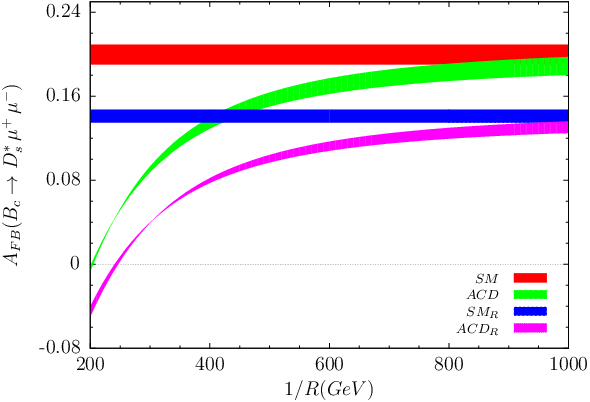
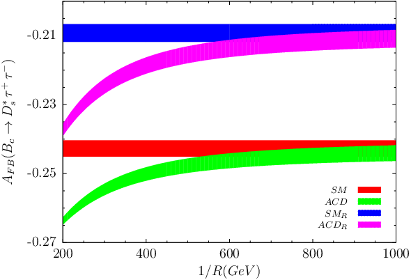
To understand the dependence of $A_{FB}$ on $1/R$ for both lepton channels better, we perform calculation at $s=0.05\,(0.4)$ for $\mu(\tau)$ and present the results in Fig. 8. In the $\mu$ channel, UED contribution on $A_{FB}$ gets important between $1/R=200-600\,GeV$, while in $\tau$ decay the contribution is insignificant for $1/R\stackrel{{\scriptstyle>}}{{{}_{\sim}}}400\,GeV$.

The position of the zero of forward-backward asymmetry, $s_{0}$, is determined numerically and the results are presented in Fig. 9. Both plots for $B_{c}\rightarrow D_{s}^{*}\mu^{+}\mu^{-}$is for the zero point in the $s<0.1$ region; the lower (upper) one is for the resonance (non resonance) case, while the zero point for $B_{c}\rightarrow D_{s}^{*}\tau^{+}\tau^{-}$is because of resonance contributions. In the SM, resonance shifts the zero point of the asymmetry, $s_{0}=0.079$, to a lower value, $s_{0}=0.068$, in $B_{c}\rightarrow D_{s}^{*}\mu^{+}\mu^{-}$, i.e., further corrections could shift $s_{0}$ to smaller values [12]. As $1/R\rightarrow 200\,GeV$ the $s_{0}$ approaches low values for both decay channels. In the $1/R=250-350\,GeV$ region, $s_{0}$ varies between ($0.058-0.068$) without resonance contributions and ($0.051-0.058$) with resonance contributions. The $s_{0}$ shift is $\sim 5\%$ of the SM value for $1/R\stackrel{{\scriptstyle>}}{{{}_{\sim}}}600\,GeV$. The variation of $s_{0}$ for $B_{c}\rightarrow D_{s}^{*}\tau^{+}\tau^{-}$is negligible.

We will discuss the possible effects of the ACD model in lepton polarization, a way of searching new physics. Using the convention followed by previous works [46]-[47], in the rest frame of $\ell^{-}$ we define the orthogonal unit vectors $S_{i}^{-}$, for the polarization of the lepton along the longitudinal, transverse and normal directions as

where $\vec{p}_{\ell}$ and $\vec{p}_{D_{s}^{\ast}}$ are the three momenta of $\ell^{-}$ and $D_{s}^{\ast}$ meson in the center of mass (CM) frame of $\ell^{+}\ell^{-}$ system, respectively. The longitudinal unit vector $S_{L}^{-}$ is boosted by Lorentz transformation,

while vectors of perpendicular directions remain unchanged under the Lorentz boost.

The differential decay rate of $B_{c}\rightarrow D_{s}^{\ast}\ell^{+}\ell^{-}$ for any spin direction $\vec{n}^{-}$ of the $\ell^{-}$ can be written in the following form

Here, $(d\Gamma/ds)_{0}$ corresponds to the unpolarized decay rate, whose explicit form is given in Eqn. (13).

The polarizations $P^{-}_{L}$, $P^{-}_{T}$ and $P^{-}_{N}$ in Eq. (20) are defined by the equation

for $i=L,~N,~T$. Here, $P^{-}_{L}$ and $P^{-}_{T}$ represent the longitudinal and transversal asymmetries, respectively, of the charged lepton $\ell^{-}$ in the decay plane, and $P^{-}_{N}$ is the normal component to both of them.

The explicit form of longitudinal polarization for $\ell^{-}$ is

Similarly, the transversal polarization is given by

and the normal polarization by

We eliminate the dependence of the lepton polarizations on $s$ in order to clarify dependence on $1/R$, by considering the averaged forms over the allowed kinematical region. The averaged lepton polarizations are defined by

References

• [1] M. S. Alam et al. (CLEO Collaboration), Phys. Rev. Lett. 74, 2885 (1995).
• [2] A. Ali, Int. J. Mod. Phys. A 20, 5080 (2005).
• [3] F. Abe et al. (CDF Collaboration), Phys. Rev. D 58, 112004 (1998).
• [4] J. Sun, Y. Yang, W. Du and H. Ma, Phys. Rev. D 77, 114004 (2008).
• [5] M. P. Altarelli and F. Teubert, Int. J. Mod. Phys. A 23, 5117 (2008).
• [6] I. Antoniadis, Phys. Lett. B 246, 377 (1990).
• [7] I. Antoniadis, N. Arkani-Hamed, S. Dimopoulos and G. Dvali, Phys. Lett. B 436, 257 (1998).
• [8] N. Arkani-Hamed, S. Dimopoulos and G. Dvali, Phys. Lett. B 429, 263 (1998).
• [9] N. Arkani-Hamed, S. Dimopoulos and G. Dvali, Phys. Rev. D 59, 086004 (1999).
• [10] T. Appelquist, H. C. Cheng and B. A. Dobrescu, Phys. Rev. D 64, 035002 (2001).
• [11] K. Agashe, N. G. Deshpande and G. H. Wu, Phys. Lett. B511, 85 (2001), B514, 309 (2001).
• [12] P. Colangelo, F. De Fazio, R. Ferrandes and T. N. Pham, Phys. Rev. D 73, 115006 (2006).
• [13] U. Haisch and A. Weiler, Phys. Rev D. 76, 034014 (2007).
• [14] P. Biancofiore, P. Colangelo and F. Fazio, arXiv:1202.2289.
• [15] T. Aaltonen, et. al., (CDF Collaboration), Phys. Rev. Lett. 107, 201802 (2011).
• [16] K. Azizi, et. al., arXiv:1203.4356.
• [17] A. J. Buras, M. Spranger and A. Weiler, Nucl. Phys. B660, 225 (2003).
• [18] A. J. Buras, A. Poschenrieder, M. Spranger and A. Weiler, Nucl. Phys. B678, 455 (2004).
• [19] P. Colangelo, F. De Fazio, R. Ferrandes and T. N. Pham, Phys. Rev. D 74, 115006 (2006).
• [20] G. Devidze, A. Liparteliani and U. G. Meissner, Phys. Lett. B 634, 59 (2006).
• [21] T. M. Aliev and M. Savci, Eur. Phys. J. C 50, 91–99 (2007).
• [22] R. Mohanta and A. K. Giri, Phys. Rev. D 75, 035008 (2007).
• [23] P. Colangelo, F. De Fazio, R. Ferrandes and T. N. Pham, Phys. Rev. D 77, 055019 (2008).
• [24] A. Saddique, M. J. Aslam and C. D. Lu, Eur. Phys. J. C 56, 267 (2008).
• [25] I. Ahmed, M. A. Paracha and M. J. Aslam, Eur. Phys. J. C 54, 591 (2008).
• [26] V. Bashiry and K. Zeynali, Phys. Rev. D 79, 033006 (2009).
• [27] N. Katirci and K. Azizi, JHEP 01, 087 (2011).
• [28] N. Katirci and K. Azizi, JHEP 07, 043 (2011).
• [29] Y. Li and J. Hua, Eur.Phys.J. C71, 1764 (2011).
• [30] U. O. Yilmaz and G. Turan, Eur. Phys. J. C 51, 63 (2007).
• [31] A. Ahmed, et. al., arXiv:1108.1058v3.
• [32] I. Ahmed, et. al., arXiv:1107.5694v2.
• [33] M. A. Paracha, I. Ahmed and M. J. Aslam, Phys. Rev. D 84, 035003 (2011).
• [34] C. Q. Geng, C. W. Hwang and C. C. Liu, Phys. Rev. D 65, 094037 (2002).
• [35] A. Faessler, Th. Gutsche, M. A. Ivanov, J. G. Körner and V. E. Lyubovitskij, Eur. Phys. J. direct C 4, 18 (2002).
• [36] D. Ebert, R. N. Faustov and V. O. Galkin, Phys. Rev. D 82, 034032 (2010).
• [37] T. Wang, D.-X., Zhang, B.-Q., Ma and T. Liu, Eur.Phys. J. C 71, 1758 (2011).
• [38] K. Azizi, F. Falahati, V. Bashiry and S. M. Zebarjad, Phys. Rev. D 77, 114024 (2008).
• [39] G. Buchalla, A. J. Buras and M. Lautenbacher, Rev. Mod. Phys. 68, 1125 (1996).
• [40] A. J. Buras and M. Münz, Phys. Rev. D 52, 186 (1995).
• [41] M. Misiak, Nucl. Phys., B393, 23 (1993), B439, 461(E) (1995).
• [42] A. Ali, T. Mannel and T. Morozumi, Phys. Lett. B 273, 505 (1991).
• [43] K. Nakamura, et al. (Particle Data Group), J. Phys. G 37, 075021 (2010).
• [44] A. Ali, P. Ball, L. T. Handoko and G. Hiller, Phys. Rev. D 61, 074024 (2000).
• [45] P. Ball and R. Zwicky, Phys. Rev. D 71, 014029 (2005).
• [46] S. Fukae, C. S. Kim and T. Yoshikawa, Phys. Rev. D 61, 074015 (2000).
• [47] F. Krüger and L. M. Sehgal, Phys. Lett. B 380, 199 (1996).
• [48] G. Erkol and G. Turan, Eur. Phys. J. C 25, 575 (2002).