跳到论文正文
W Papers独立论文阅读器 arXiv:1204.1253 论文正文 计算阅读时间 · 0%
引用这篇论文根据当前论文元数据生成,正式投稿前建议核对。


License: arXiv.org perpetual non-exclusive license
arXiv:1204.1253v2 [math-ph] 26 Apr 2013

The scaling limit of polymer pinning dynamics and a one dimensional Stefan freezing problem

Hubert Lacoin
Abstract.

We consider the stochastic evolution of a 1+11+1-dimensional interface (or polymer) in presence of a substrate. This stochastic process is a dynamical version of the homogeneous pinning model. We start from a configuration far from equilibrium: a polymer with a non-trivial macroscopic height profile, and look at the evolution of a space-time rescaled interface. In two cases, we prove that this rescaled interface has a scaling limit on the diffusive scale (space rescaled by LL in both dimensions and time rescaled by L2L^{2} where LL denotes the length of the interface) which we describe: when the interaction with the substrate is such that the system is unpinned at equilibrium, then the scaling limit of the height profile is given by the solution of the heat equation with Dirichlet boundary condition ; when the attraction to the substrate is infinite, the scaling limit is given a free-boundary problem which belongs to the class of Stefan problems with contracting boundary, also referred to as Stefan freezing problems. In addition, we prove the existence and regularity of the solution to this problem until a maximal time, where the boundaries collide.
2010 Mathematics Subject Classification: 82C24, 80A22, 60F99.
Keywords: Heat-bath dynamics, Scaling Limit, Stefan Problem, Interface Motion, Pinning model.

1. Introduction

1.1. The dynamical pinning model

Random polymer models have been used for a long time by physicists to describe a large variety of physical phenomena. Among the numerous models that have been introduced by theoretical physicists and rigorously studied by mathematicians (see e.g. [13] for a survey of the most studied polymer models), the polymer pinning model, that involves a simple random walk interacting with a defect line, has focused a lot of interest both of the mathematics and physics community. The phase transition phenomenon between a pinned phase and a depinned one is now well understood, even in presence of disorder (see [9] for a seminal paper concerning the homogeneous case, and [10, 11] for recent reviews).

On the other hand, dynamical pinning (which has some importance in biophysical application see [1, 2] and references therein) has attracted attention of mathematicians only more recently and a lot of questions concerning relaxation to equilibrium and its connection properties are still unsolved.

The object of most of the mathematical studies on the dynamical pinning model up to now (see [3, 4]) has been the mixing time and the relaxation time for the dynamics. It has been shown there that the mixing property of the system depends in a crucial way of the pinning parameter λ\lambda, or more precisely, on whether the polymer at equilibrium is pinned or unpinned.

In the present paper, we choose to study a different aspect, that is, the dynamical scaling limit of the height-profile of the polymer. We start from an initial condition that is very far from equilibrium and approximates a macroscopic deterministic profile and we want to describe the evolution of the profile under diffusive scaling. Our aim is to show that the nature of the limit of the rescaled process depends only on whether one lies in the pinned or depinned phase, and to describe explicitly the scaling limit in each case.

The scaling limit is easier to guess in the unpinned phase. As in this case, there is no contact point with the substrate at equilibrium, one can infer that the scaling limit is the same that for a system with no substrate, for which it is known that the height profile converges to the solution of the heat-equation on the segment with zero Dirichlet boundary condition.

In the pinned phase, a more interesting phenomenon takes place. In this case the dynamical picture should be the following: there are macroscopic region where the polymer is pinned to the substrate and other regions where the polymer stays at a macroscopic distance from it; the boundary between the pinned and the unpinned region is moving in time and in the unpinned region, the polymer profile evolves according to the heat-equation. The system reaches equilibrium when the unpinned region has totally vanished.

In the present paper, we prove that this picture holds when the pinning parameter is infinite (or tending to infinity sufficiently fast with the size of the system). An important step to establish this result is to prove existence and regularity of the free-boundary problem that appears in the scaling limit.

1.2. A one dimensional Stefan freezing problem

The free-boundary problem of unknown (f,l,r)(f,l,r) (ff is the function and ll and rr are the boundary of the unpinned region) that appears as the scaling limit of the pinning model in the pinned phase is the following

{∂tf−fx​x=0on ​(l⁡(t),r⁡(t)),f⁡(⋅,t)≡0on ​[−1,1]∖(l⁡(t),r⁡(t)),fx​(l⁡(t),t)=−fx​(r⁡(t),t)=1,l′(t)=−fx​x(l(t),t),r′(t)=fx​x(r(t),t),f(⋅,0)=f0,l(0)=l0,r0.\begin{cases}\partial_{t}f-f_{xx}=0\quad\text{on }(l(t),r(t)),\\ f(\cdot,t)\equiv 0\quad\text{on }[-1,1]\setminus(l(t),r(t)),\\ f_{x}(l(t),t)=-f_{x}(r(t),t)=1,\\ l^{\prime}(t)=-f_{xx}(l(t),t),\quad r^{\prime}(t)=f_{xx}(r(t),t),\\ f(\cdot,0)=f_{0},\ l(0)=l_{0},\ r_{0}.\end{cases} (1.1)

We are exclusively interested in the case of a 11-Lipshitz initial condition that vanishes outside of the interval (r0,l0)⊂[−1,1](r_{0},l_{0})\subset[-1,1] and is positive inside. This problem belongs to the class of Stefan problem, which have been introduced in mathematics to describe the evolution of a multiphase medium.

The boundary condition for fxf_{x} and the fact that the heat equation preserves Lipshitzianity imply that ff cannot be convex in the neighborhood of the moving boundaries, and thus the boundary points l⁡(t)l(t) and r⁡(t)r(t) are moving towards each other (l′​⩾​ 0l^{\prime}\;\geqslant\;0 and r′​⩾​ 0r^{\prime}\;\geqslant\;0). These problems with contracting boundary are referred to as freezing problems whereas those with expanding boundary are called melting problems.

Most of the work in the literature on Stefan problems concerns melting problems. One of the reason for this is that these problem can be rewritten as a diffusion equation for an enthalpy function with a diffusion coefficient that is monotonous increasing function of the enthalpy. This monotonicity allows to derive uniqueness of the solution with some generality (we refer to the Introduction of [7] for more precision). The freezing problems like (1.1) on the contrary are more challenging even in the one dimensional setup.

Even though one dimensional freezing problems have attracted some attention in a recent past [5, 6], some amount of work is required to establish the existence and the unicity of a solution to (1.1) up to a maximal time.

2. Model and results

2.1. A simple model for interface motion with no constraint

To introduce our reader to polymer dynamics, we first introduce the simplest version of the model where no substrate is present: this is the so-called corner-flip dynamics. Let Ω=ΩL\Omega=\Omega_{L} denote the set of all lattice paths (polymers) starting at 00 and ending at 00 after 2​L2L steps

ΩL0:={η∈ℤ2​L+1|η−L=ηL=0,|ηx+1−ηx|=1,x=−L,…,L−1}.\Omega^{0}_{L}:=\{\eta\in{\mathbb{Z}}^{2L+1}\ |\ \eta_{-L}=\eta_{L}=0\,,\;|\eta_{x+1}-\eta_{x}|=1,\;x=-L,\dots,L-1\}\,. (2.1)

The stochastic dynamics is defined by the natural spin-flip continuous time Markov chain with state space ΩL0\Omega^{0}_{L}. Namely, sites x=−L,…,Lx=-L,\dots,L are equipped with independent Poisson clocks which ring with rate one: when a clock rings at xx the path η\eta is replaced by η(x)\eta^{(x)}, defined by ηy(x)=ηx(x)\eta_{y}^{(x)}=\eta_{x}^{(x)} for all y≠xy\neq x and

ηx(x):={ηx+2​ if ​ηx±1=ηx+1,ηx−2​ if ​ηx±1=ηx−1,ηx​ if ​|ηx+1−ηx−1|=2.\eta_{x}^{(x)}:=\begin{cases}\eta_{x}+2\text{ if }\eta_{x\pm 1}=\eta_{x}+1,\\ \eta_{x}-2\text{ if }\eta_{x\pm 1}=\eta_{x}-1,\\ \eta_{x}\text{ if }|\eta_{x+1}-\eta_{x-1}|=2.\end{cases} (2.2)

One denotes by (η~​(⋅,t)\widetilde{\eta}(\cdot,t), t​⩾​ 0t\;\geqslant\;0), the trajectory of the Markov chain. By doing linear interpolation between the integer values of xx, one can consider η~​(⋅,t)\widetilde{\eta}(\cdot,t) as a function of the real variable x∈[−L,L]x\in[-L,L].

The unique invariant measure for this dynamics is the uniform measure on ΩL0\Omega^{0}_{L}, and thus, from standard properties of the random walk, when the system is at equilibrium, the rescaled interface (η⁡(L​x)/L)x∈[−1,1](\eta(Lx)/L)_{x\in[-1,1]} is macroscopically flat (η⁡(x)\eta(x) has fluctuation of order L\sqrt{L}). For this model, relaxation to equilibrium is well understood both in terms of mixing-time (see Wilson [20]) or scaling limits (see [15, Theorem 3.2], weaker versions of these result had been known before, using connection with the one dimensional simple symmetric exclusion process).

We cite in full the result concerning the scaling limit for two reasons: it gives some point of reference to better understand results in presence of a substrate; and we use it as a fundamental building brick for the proof of our new results.

Given f0f_{0} a Lipshitz function in [−1,1][-1,1], with f0​(−1)=f0​(1)=0f_{0}(-1)=f_{0}(1)=0, set f~\widetilde{f} defined on [−1,1]×[0,∞)[-1,1]\times[0,\infty) to be the solution of the heat equation with Dirichlet boundary condition

{∂tf~−f~x​x=0,f~​(⋅,0)=f0,f~​(−1,t)=f~(1,t)=0,∀t>0.\begin{cases}\partial_{t}\widetilde{f}-\widetilde{f}_{xx}&=0,\\ \widetilde{f}(\cdot,0)&=f_{0},\\ \widetilde{f}(-1,t)&=\widetilde{f}(1,t)=0,\quad\forall t>0.\end{cases} (2.3)
Theorem 2.1 ([15] Theorem 3.2).

Let η~L\widetilde{\eta}^{L} be the dynamic described above, starting from a sequence of initial condition η0L\eta^{L}_{0} that satisfies,

η0L​(x)=L⁡(f0​(x/L)+o⁡(1))​ uniformly in x when L→∞ .\eta^{L}_{0}(x)=L(f_{0}(x/L)+o(1))\text{ uniformly in $x$ when $L\to\infty$ }. (2.4)

Then, under diffusive scaling, η~L\widetilde{\eta}^{L} converges to f~\widetilde{f} in law for the uniform topology: for any T>0T>0, in probability,

limL→∞supx∈[−1,1],t∈[0,T]|1L​η~L​(L​x,L2​t)−f~​(x,t)|=0.\lim_{L\to\infty}\sup_{x\in[-1,1],t\in[0,T]}\left|\frac{1}{L}\widetilde{\eta}^{L}(Lx,L^{2}t)-\widetilde{f}(x,t)\right|=0. (2.5)

The notation in Equation (2.4) means that there exists a function εL\varepsilon_{L} tending to zero such that for all xx and LL

|η0L​(x)−L⁡(f0​(x/L))L|​⩽​εL.\left|\frac{\eta^{L}_{0}(x)-L(f_{0}(x/L))}{L}\right|\;\leqslant\;\varepsilon_{L}. (2.6)

We keep this notation for the rest of the paper.

2.2. Dynamical polymers interacting with a substrate

Let us now define precisely the model that is the object of study of this paper. Our aim is to understand how the pattern of relaxation to equilibrium given by Theorem 2.1 is modified (or not modified) when the dynamics has additional constraints. We focus on the case of an interface interacting with a solid substrate. This brings us to consider a dynamics with the following modifications:

  • •

    We consider that a solid wall fills the entire bottom half-plane so that our trajectories have to stay in the positive half-plane (ηx​⩾​ 0\eta_{x}\;\geqslant\;0, ∀x∈{−L,…,L}\forall x\in\{-L,\dots,L\}).

  • •

    The wall interacts with the interface η\eta so that the rates of the transitions that modifies the number of contacts with the wall are changed.

More precisely one starts from a trajectory that lies entirely above the wall, i.e. which belongs to the following subset of ΩL0\Omega_{L}^{0}:

ΩL:={η∈ℤ2​L+1|η−L=ηL=0;∀x∈{−L,…,L−1},|ηx+1−ηx|=1,ηx⩾ 0}.\Omega_{L}:=\{\eta\in{\mathbb{Z}}^{2L+1}\ |\;\eta_{-L}=\eta_{L}=0\,;\ \forall x\in\{-L,\dots,L-1\},\ |\eta_{x+1}-\eta_{x}|=1,\eta_{x}\;\geqslant\;0\}\,. (2.7)

The rates of the transitions from η\eta to η(x)\eta^{(x)} are not uniformly equal to 11 as in the previous section but they are given by

c⁡(η,η(x))={0​ if ​ηx(x)=−1(interdiction to go through the wall),2​λ1+λ​ if ​ηx=2​ and ​ηx(x)=0,21+λ​ if ​ηx=0​ and ​ηx(x)=2,1​ in every other cases .c(\eta,\eta^{(x)})=\begin{cases}0\text{ if }\eta_{x}^{(x)}=-1\quad\text{(interdiction to go through the wall)},\\ \frac{2\lambda}{1+\lambda}\text{ if }\eta_{x}=2\text{ and }\eta_{x}^{(x)}=0,\\ \frac{2}{1+\lambda}\text{ if }\eta_{x}=0\text{ and }\eta_{x}^{(x)}=2,\\ 1\text{ in every other cases }.\end{cases} (2.8)

The generator ℒ=ℒLλ\mathcal{L}=\mathcal{L}^{\lambda}_{L} of the Markov process is given by

ℒ⁡(f)=∑x=−L+1L−1c⁡(η,η(x))​(f⁡(η(x))−f⁡(η)CLOSE.\mathcal{L}(f)=\sum_{x=-L+1}^{L-1}c(\eta,\eta^{(x)})(f(\eta^{(x)})-f(\eta). (2.9)

The value of the parameter λ∈[0,∞]\lambda\in[0,\infty] determines the nature of the interaction with the wall. If λ>1\lambda>1, the transitions adding a contact are favored, which means that the wall is attractive, whereas if λ<1\lambda<1 the wall is repulsive.

The process defined above is the heat-bath dynamics for the polymer pinning model, with equilibrium measure π=π2​Lλ\pi=\pi_{2L}^{\lambda} on ΩL\Omega_{L} defined by

πLλ​(η)=λN⁡(η)Z2​Lλ,\pi^{\lambda}_{L}(\eta)=\frac{\lambda^{N(\eta)}}{Z_{2L}^{\lambda}}\,, (2.10)

where

N⁡(η)=#⁡{x∈[−L+1,L−1]:ηx=0}N(\eta)=\#\{x\in[-L+1,L-1]\,:\;\eta_{x}=0\}

denotes the number of zeros in the path η∈Ω\eta\in\Omega and

Z2​Lλ:=∑η′∈ΩLλN⁡(η′)Z_{2L}^{\lambda}:=\sum_{\eta^{\prime}\in\Omega_{L}}\lambda^{N(\eta^{\prime})} (2.11)

is the partition function, which is the renormalization factor that makes πLλ\pi_{L}^{\lambda} a probability.

For every λ>0\lambda>0, L∈ℕL\in{\mathbb{N}}, πLλ\pi_{L}^{\lambda} is the unique reversible invariant measure for the Markov chain. For any value of λ\lambda, the rescaled version of η\eta at equilibrium (that is, under the measure πLλ\pi_{L}^{\lambda}) is flat, but the microscopic properties of η\eta vary with the value of λ\lambda:

  • (i)

    When λ∈[0,2)\lambda\in[0,2), the interface is repelled by the wall (i.e. when λ∈(1,2)\lambda\in(1,2), the entropic repulsion wins against the energetic attraction of the wall) and typical paths have a number of contacts with the wall which stays bounded when LL tends to infinity (the sequence of the laws of N⁡(η)N(\eta) is tight).

  • (ii)

    When λ∈(2,∞]\lambda\in(2,\infty], the interface is pinned to the wall, and typical paths have a number of contacts with the wall which is of order LL.

  • (iii)

    When λ=2\lambda=2, η\eta has a lot of contact with the wall (order L\sqrt{L}) but the longest excursion away from the wall has length of order LL.

For more precise statements and proofs, we refer to Chapter 2 in [10]. These three cases are respectively referred to as the depinned or unpinned phase, the pinned phase, and the critical point (or phase transition point).

Remark 2.2.

The case λ=∞\lambda=\infty, that will be also considered in this paper is a bit particular. Indeed, as seen in (2.8), when ηx=0\eta_{x}=0 (when η\eta touches the wall at xx), it sticks to it forever, so that η⁡(⋅,t)\eta(\cdot,t) stops moving once it has reached the minimal configuration ηmin\eta^{\min} defined by

ηxmin:={0​ if ​x+L​ is even ,1​ if ​x+L​ is odd ,\eta^{\min}_{x}:=\begin{cases}0\text{ if }x+L\text{ is even },\\ 1\text{ if }x+L\text{ is odd },\end{cases} (2.12)

which is the configuration with the maximal number of contact point with the wall. In that case, the unique invariance probability measure is the Dirac mass on ηmin\eta^{\min}. A question of interest is then to compute the time at which η⁡(⋅,t)\eta(\cdot,t) stops to move: the hitting time of ηmin\eta^{\min}.

Our aim is to get a result similar to Theorem 2.1, describing how, starting from a non-flat profile, the system relaxes to equilibrium. We are able to deduce results in two cases:

  • •

    in the depinned phase, when λ∈[0,2)\lambda\in[0,2): in that case the scaling limit is the same one as for the model without wall. The result can be obtained with rather soft comparison arguments when λ​⩽​ 1\lambda\;\leqslant\;1 but requires some additional work when λ∈(1,2)\lambda\in(1,2).

  • •

    when the wall is sticky, λ=∞\lambda=\infty: in that case, the attraction of the wall can be seen ot the macroscopic level, and the scaling limit is given by the solution of a partial differential equation with moving boundary: the free bounary problem (1.1).

We can understand what happens when λ=2\lambda=2 (the critical point) and when λ∈(2,∞)\lambda\in(2,\infty) (the pinned phase) at a heuristic level, and formulate this as conjectures (see Section 2.7). There are a lot of technical reasons why bringing these conjectures to rigorous ground cannot be done only we the ideas exposed in this paper. We might address this issue in future work.

2.3. Scaling limit in the repulsive case

Our first result is an analog of Theorem 2.1 for the dynamic in the depinned phase.

Theorem 2.3.

Let η=ηL,λ\eta=\eta^{L,\lambda} be the dynamic on ΩL\Omega_{L} with generator ℒ\mathcal{L} described above, with the parameter λ∈[0,2)\lambda\in[0,2) and starting from a sequence of initial condition η0L\eta^{L}_{0} satisfying

η0L​(x)=L​f0​(x/L)​(1+o⁡(1))​ uniformly in x when L→∞ ,\eta^{L}_{0}(x)=Lf_{0}(x/L)(1+o(1))\text{ uniformly in $x$ when $L\to\infty$ }, (2.13)

where f0f_{0} is a 11-Lipshitz non-negative function.

Then ηL,λ\eta^{L,\lambda} converges to f~\widetilde{f} defined by (2.3) in law for the uniform topology in the sense that for any T>0T>0,

limL→∞supx∈[−1,1],t∈[0,T]|1L​ηL​(L​x,L2​t)−f~​(x,t)|=0,\lim_{L\to\infty}\sup_{x\in[-1,1],t\in[0,T]}\left|\frac{1}{L}\eta^{L}(Lx,L^{2}t)-\widetilde{f}(x,t)\right|=0, (2.14)

in probability.

This result is not much of a surprise. For this range of λ\lambda, the wall is pushing the trajectory η\eta away, so that for most of the time η⁡(t)\eta(t) lies in the wall-free zone. This is the reason why the effect of the wall does not appear in the scaling limit. We believe that this also to be the case for λ=2\lambda=2, but the fact that L\sqrt{L} contact with the wall can appear at equilibrium instead of O⁡(1)O(1) brings an additional technical challenge.

2.4. Toward the scaling limit for pinning on a sticky substrate

We move now to the case λ=∞\lambda=\infty. In that case (recall (2.8)), the corners on the interface flip with rate 11 if it does not change the number of contact with the wall, with rate 22 if it adds one contact, and the contacts with the wall cannot be removed and stay forever. In that case, it is known that with large probability after a time L2L^{2} the dynamics ends up with a path completely stuck to the substrate (with probability tending to 11), (see [3, Proposition 5.6] or Lemma 6.1 below). This implies in particular that the scaling limit in this case cannot be given by (2.3).

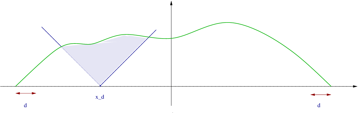
Let us try to give some heuristic justification for the PDE problem that rules the evolution of scaling limit ff. We suppose that the polymer path consists of a pinned region where it sticks to the wall and f≡0f\equiv 0 and an unpinned region which corresponds to an interval [L​l​(t),L​r​(t)][Ll(t),Lr(t)] (i.e. (l⁡(t),r⁡(t))(l(t),r(t)) for the rescaled picture) so that f⁡(t,l⁡(t))=f⁡(t,r⁡(t))=0f(t,l(t))=f(t,r(t))=0. In the unpinned region the wall has no influence and thus Theorem 2.1 indicates that one should have ∂tf−fx​x=0\partial_{t}f-f_{xx}=0. What is left to be determined is the speed at which the boundary of the pinned region moves (value of of the time derivative l′​(t)l^{\prime}(t) and r′​(t)r^{\prime}(t)) and/or the boundary condition that ff has to satisfy at the boundary of (l⁡(t),r⁡(t))(l(t),r(t)).

Remark 2.4.

With the boundary condition that one considers, ff is not space derivable at the extremities of [l⁡(t),r⁡(t)][l(t),r(t)]. In what follows, when one talk about the space derivatives of ff at point l⁡(t)l(t), resp. r⁡(t)r(t), we refer to right resp. left derivatives.

What we want to justify here is that the slope of the scaling limit at the left (resp. right) boundary of the pinned region, given by fx​(l​(t),t)f_{x}(l(t),t) (resp. fx​(r​(t),t)f_{x}(r(t),t)) has to be equal to +1+1 (resp. −1-1). The reason for this is that, as the scaling is diffusive, the mean-speed of the left-boundary of the pinned zone for the non-rescaled dynamics has to be of order 1/L1/L. This can be achieved only if the density of down-steps near the left boundary is vanishing, and hence if fx​(l​(t),t)=1f_{x}(l(t),t)=1.

Combining this boundary condition with ∂tf−fx​x\partial_{t}f-f_{xx}, and doing some trigonometry it implies (at least at the heuristic level) that one must also have l′​(t)=−fx​x​(t,l⁡(t))l^{\prime}(t)=-f_{xx}(t,l(t)) and r′​(t)=fx​x​(t,l⁡(t))r^{\prime}(t)=f_{xx}(t,l(t)). Thus, ff should be the solution of (1.1).

2.5. Solving the Stefan problem

The problem (1.1) is slightly overdetermined but this obstacle vanishes if one considers the derivative problem,

{∂tρ−ρx​x​ in (l⁡(t);r⁡(t)),ρ⁡(l⁡(t),t)≡1​ on ​[−1,l⁡(t)],ρ⁡(r⁡(t),t)=−1​ on ​[l⁡(t),1]l′(t)=−ρx(l(t),t),r′(t)=ρx(r(t),t),ρ⁡(⋅,0)=ρ0​ on ​(r0,l0).\begin{cases}\partial_{t}\rho-\rho_{xx}\text{ in }\quad\left(l(t);r(t)\right),\\ \rho(l(t),t)\equiv 1\text{ on }[-1,l(t)],\quad\rho(r(t),t)=-1\text{ on }[l(t),1]\\ l^{\prime}(t)=-\rho_{x}(l(t),t),\quad r^{\prime}(t)=\rho_{x}(r(t),t),\\ \rho(\cdot,0)=\rho_{0}\text{ on }(r_{0},l_{0}).\end{cases} (2.15)

A problem very similar to (2.15) has been considered by Chayes and Kim in [5] but with the third line replaced by

l′(t)=−ρx(l(t),t)/2 and r′(t)=ρx(r(t),t)/2.l^{\prime}(t)=-\rho_{x}(l(t),t)/2\text{ and }r^{\prime}(t)=\rho_{x}(r(t),t)/2.

Note that the formulation in [5] is slightly differs but this is what one finds after appropriate rescaling). This small change has big consequences on the behavior of the solution. Whereas for the problem considered by [5], the solution exists until a maximal time where r⁡(t)=l⁡(t)r(t)=l(t) for all reasonable initial condition ρ0\rho_{0}, our problem might show some degeneracy when ll and rr are still well apart (see Section 3.2).

What we show in this paper is that this kind of complication does not occur for the initial conditions we are interested in. Furthermore, we establish regularity and further additional properties of interest.

Theorem 2.5.

Suppose that f0f_{0} is a 11-Lipshitz function positive and smooth on (l0,r0)(l_{0},r_{0}) and satisfies the boundary condition f′​(l0)=−f′​(r0)=1f^{\prime}(l_{0})=-f^{\prime}(r_{0})=1. Then the free boundary problem (1.1) has a unique classical solution up to time

T∗=12​∫l0r0f⁡(x)​d​x,T^{*}=\frac{1}{2}\int^{r_{0}}_{l_{0}}f(x)\,\text{\rm d}x,

at which the area below the curve vanishes.

Furthermore:

  • (i)

    r⁡(t)r(t) and l⁡(t)l(t) are C∞C^{\infty} on on the interval (0,T∗)(0,T^{*}),

  • (ii)

    ff becomes concave on (l⁡(t),r⁡(t))(l(t),r(t)) before time T∗T^{*},

  • (iii)

    limt→T∗(r⁡(t)−l⁡(t))=0\lim_{t\to T^{*}}(r(t)-l(t))=0.

Equivalently if ρ0\rho_{0} is the derivative of a function f0f_{0} that has the above properties, then (2.15) has a solution until time T∗T^{*} where the two boundary meets.

The proof of short-time existence and regularity of the boundary motion strongly relies on the work and Kim and Chayes [6], and does not require ρ0\rho_{0} to be the derivative of positive function, but just reasonable regularity assumption (we suppose it Lipshitz but this could be relaxed).

The proof of existence until a maximal time uses ideas and is inspired by the work of Grayson concerning the shrinking of curves by curvature flow [12].

2.6. The scaling limit for λ=∞\lambda=\infty

We are now ready to state our result concerning the dynamics with a wall and λ=∞\lambda=\infty.

Theorem 2.6.

Let ηL,∞\eta^{L,\infty} denote the dynamic with wall and λ=∞\lambda=\infty, and starting from a sequence of initial condition η0L\eta^{L}_{0} which satisfies

η0L​(x)=L​f0​(x/L)​(1+o⁡(1))​ uniformly in x when L→∞ ,\eta^{L}_{0}(x)=Lf_{0}(x/L)(1+o(1))\text{ uniformly in $x$ when $L\to\infty$ }, (2.16)

where f0f_{0} satisfies the assumption of Theorem 2.5. Set ff to be the solution of (1.1).

Then ηL,∞\eta^{L,\infty} converges to ff in law for the uniform topology in the sense that

limL→∞supx∈[−1,1],t>0|1L​ηL,∞​(L​x,L2​t)−f⁡(x,t)|=0,\lim_{L\to\infty}\sup_{x\in[-1,1],t>0}\left|\frac{1}{L}\eta^{L,\infty}(Lx,L^{2}t)-f(x,t)\right|=0, (2.17)

in probability.

Moreover, one can precisely estimate the time at which the dynamics terminates

𝒯:=inf{t​⩾​ 0|η⁡(⋅,t)=ηmin}.\mathcal{T}:=\inf\{t\;\geqslant\;0\ |\ \eta(\cdot,t)=\eta^{\min}\}. (2.18)

We have that in probability

limL→∞𝒯L2=∫01f0​(x)​d​x.\lim_{L\to\infty}\frac{\mathcal{T}}{L^{2}}=\int_{0}^{1}f_{0}(x)\,\text{\rm d}x. (2.19)

The second part of the result (2.18) can be compared to the result obtained by Caputo et al. [3, Theorem 5.5 and Proposition 5.6], where is proved that the mixing time for this dynamics is of order L2L^{2}.

Remark 2.7.

The assumption that ff is strictly positive in (l0,r0)(l_{0},r_{0}) is necessary and if ff cancels in the middle of the interval, the scaling limit depends on the microscopic details of the initial condition and the scaling limit might be a random object even for a deterministic initial condition.

2.7. Discussion on the scaling limit in the attractive case for λ∈(2,∞)\lambda\in(2,\infty)

Although we are quite far from being able to prove it, we do believe that Theorem 2.6 extends in some way to the whole localized phase λ∈(2,∞)\lambda\in(2,\infty). We summarize here the full conjecture and give an idea of the technical difficulties that arises when trying to prove it.

What we believe is that the polymer consists of one (or several) unpinned region situated a macroscopic distance of the interface, and pinned regions where the polymers looks locally at equilibrium (recall that when λ>2\lambda>2 the polymer has a density of contacts for πLλ\pi^{\lambda}_{L}. As before it is natural to say that in the unpinned region, the rescaled polymer must satisfy ∂f−fx​x=0\partial f-f_{xx}=0. However, the argument giving the slope of ff at the boundary of the unpinned region in the λ=∞\lambda=\infty case is not valid when λ\lambda is finite, because the boundary can now microscopically move in both direction as unpinning is allowed.

To guess the value of the slope at the boundary ∂xf⁡(t,l⁡(t))\partial_{x}f(t,l(t)), ∂xf⁡(t,r⁡(t))\partial_{x}f(t,r(t)), we assume that the system close to the phase separation must be in a state of local-equilibrium.

From the equilibrium results on polymer pinning with elevated boundary condition proved in [16], one can infer that the equilibrium slope of a polymer at the boundary of a pinned and an unpinned phase is

dλ:=1−2λ.d_{\lambda}:=1-\frac{2}{\lambda}.

and that one must have

fx​(t,l⁡(t))=−fx​(t,r⁡(t))=dλ.f_{x}(t,l(t))=-f_{x}(t,r(t))=d_{\lambda}.

Hence, the scaling limit ff of ηL,λ​(x,t)\eta^{L,\lambda}(x,t) with λ>2\lambda>2 must satisfy the following free boundary problem

{∂tf−fx​x=0on ​(l⁡(t),r⁡(t)),f⁡(⋅,t)≡0on ​[−1,1]∖(l⁡(t),r⁡(t)),fx​(l⁡(t),t)=−fx​(r⁡(t),t)=dλ,l′(t)=−fx​x(l(t),t)/dλ,r′(t)=fx​x(r(t),t)/dλ,f(⋅,0)=f0,l(0)=l0,r0.\begin{cases}\partial_{t}f-f_{xx}=0\quad\text{on }(l(t),r(t)),\\ f(\cdot,t)\equiv 0\quad\text{on }[-1,1]\setminus(l(t),r(t)),\\ f_{x}(l(t),t)=-f_{x}(r(t),t)=d_{\lambda},\\ l^{\prime}(t)=-f_{xx}(l(t),t)/d_{\lambda},\quad r^{\prime}(t)=f_{xx}(r(t),t)/d_{\lambda},\\ f(\cdot,0)=f_{0},\ l(0)=l_{0},\ r_{0}.\end{cases} (2.20)

The problem (2.20) presents additional technical difficulties when compared to (1.1), even though the difference between them is just a scaling factor. The reason for this is comes from the kind of initial condition that one wants to consider. If one starts from an initial condition that is positive in (l0,r0)(l_{0},r_{0}) and Lipshitz with Lipshitz constant dλd_{\lambda}, then Theorem 2.5 ensures that the solution to (2.20) exists and is well behaved until the time when the pinned region has vanished. However, if one consider a 11-Lipshitz boundary condition, fx​x​(l​(t),t)f_{xx}(l(t),t) can be positive for some times, and thus the boundary are not necessarily contracting… which makes the problem more difficult to solve.

When the wall is sticky, there is no loss of generality in considering that there is only one unpinned region, because two regions separated by a contact with the wall stay separated and behave independently. When λ<∞\lambda<\infty the situation is different: if one starts with two distinct unpinned regions (l1,r1)(l_{1},r_{1}) and (l2,r2)(l_{2},r_{2}) with l2>r1l_{2}>r_{1}, this is possible that the two region merge at a positive time.

Besides these obstacles on the analytical side, there are many reasons why the proof of Theorem 2.6 cannot easily be adapted to the case λ∈(2,∞)\lambda\in(2,\infty). Indeed a part of the strategy relies on the control of the area below η\eta (see for instance Lemma 6.1) and this kind of argument seems very difficult to adapt when the polymer is allowed to detach itself from the wall.

2.8. Stefan problem and statistical mechanics

Free boundary problems similar to (2.15) appear naturally in thermodynamics to describe the motion of phase boundary in a multiphase medium (e.g. water in solid and liquid state), and for this reason have been the object of extensive studies (see the seminal paper of Stefan [19] and [18] for a survey the subject).

There has been then some recent efforts in the area of statistical mechanics in order to prove to show that Stefan problem can be obtained as the limiting equation of evolution for particle systems whose microscopic behavior is random. Among these work we can cite [7], where Chayes and Swindle have exhibited a particle system whose hydrodynamic limit is given by a Stefan problem, and [17] where Landim and Valle proposed a microscopic modeling of Stefan freezing/melting problem and proved the weak convergence of the particle density to the solution of a free boundary equation (for a more complete bibliography we refer to the monograph [14]).

The main difference of the problem we study here when compared to the one considered e.g. in [7] and [17] is that, microscopically, the motion of the phase boundary does not depend only on the state of the system close to the boundary, but on the whole configuration (a contact to the wall can be added anywhere and not only near the boundary). This makes control of the boundary motion more difficult, and for this reason we did not use an approach based on weak convergence like in most of the literature, but something based on a classical interpretation of the partial differential equations. This is the reason why we have to prove the existence of a solution of (2.15) first: we cannot prove a convergence result a priori without knowing about the existence of a classical (and sufficiently regular) solution.

After a preliminary version of this paper was published, De Masi et al. [8] proved a convergence result for a special version of the simple exclusion process with moving sources and sinks at the boundary. They conjecture that the scaling limit they obtain is a solution of a problem similar to (1.1), but for which there exists a stationary solution.

2.9. Organization of the paper

In Section 3 we prove Theorem 2.5. In Section 4, we introduce a few result to that will be of use both for the proof of Theorem 2.3 and 2.6. In Section 5 we prove Theorem 2.3. Finally Section 6 contains the proof of Theorem 2.6

3. Proof of Theorem 2.5

3.1. Decomposition of the proof

To prove the result we proceed in three steps. Firstly, we use results and ideas from [6] to prove the existence and the unicity of a C∞C^{\infty} solution for a short-time, and to extend this solution until a time where the second derivative of ff becomes unbounded.

Proposition 3.1.

If f0f_{0} is smooth and Lipshitz on [l0,r0][l_{0},r_{0}] and satisfies the boundary condition f′​(l0)=−f′​(r0)=1f^{\prime}(l_{0})=-f^{\prime}(r_{0})=1. Then there exists t1t_{1} dor which the problem (1.1) has a classical solution on [0,t1)[0,t_{1}) which satisfies

limt→t1supx∈(l⁡(t),r⁡(t))|fx​x​(x,t)|=∞.\lim_{t\to t_{1}}\sup_{x\in(l(t),r(t))}|f_{xx}(x,t)|=\infty. (3.1)

Furthermore l⁡(t)l(t) and r(t)(t) are C∞C_{\infty} on (0,t1)(0,t_{1}).

Then we show that if f0f_{0} restricted to (l0,r0)(l_{0},r_{0}) is a concave function, the solution exists up to a maximal time where the boundaries ll and rr meet.

Proposition 3.2.

If f0f_{0} is concave on (l0,r0)(l_{0},r_{0}), then

t1=T∗=∫l0r0f0​(x)​d​x/2t_{1}=T^{*}=\int^{r_{0}}_{l_{0}}f_{0}(x)\,\text{\rm d}x/2

and

limt→T∗(r⁡(t)−l⁡(t))=0.\lim_{t\to T^{*}}(r(t)-l(t))=0.

Finally, we show that if f0f_{0} is positive, then it becomes concave before t1t_{1}.

Proposition 3.3.

If f0f_{0} is positive, then there exists a time t2<t1t_{2}<t_{1} such that f⁡(⋅,t)f(\cdot,t) is concave for t∈[t2,t1)t\in[t_{2},t_{1}).

Theorem 2.5 is obtained by combining the three statements together.

3.2. Discussion on the case of general f0f_{0}

Before going into the proofs, let us first discuss about why the positivity of ff is required for the existence of a solution until T∗T^{*}. We show in this section with simple examples that if this condition is violated, the solution might degenerate and the boundary condition can stop being satisfied before l⁡(t)l(t) and r⁡(t)r(t) meet.

First note that the fact that the area below the curve vanishes at T∗T^{*} is a simple consequence of

∂t(∫l⁡(t)r⁡(t)f⁡(x,t)​d​x)=∫l⁡(t)r⁡(t)fx​x​(x,t)​d​x=fx​(l⁡(t),t)−fx​(r⁡(t),t)=−2.\partial_{t}\left(\int_{l(t)}^{r(t)}f(x,t)\,\text{\rm d}x\right)=\int_{l(t)}^{r(t)}f_{xx}(x,t)\,\text{\rm d}x=f_{x}(l(t),t)-f_{x}(r(t),t)=-2. (3.2)

so that for all t∈(0,t1)t\in(0,t_{1}) for which the solution is defined

∫l⁡(t)r⁡(t)f⁡(x,t)​d​x=∫l⁡(t)r⁡(t)f0​(x)​d​x−2​t.\int_{l(t)}^{r(t)}f(x,t)\,\text{\rm d}x=\int_{l(t)}^{r(t)}f_{0}(x)\,\text{\rm d}x-2t. (3.3)

Thus if f0f_{0} is such that ∫l⁡(t)r⁡(t)f0​(x)<0\int_{l(t)}^{r(t)}f_{0}(x)<0 and satisfies the assumption of Proposition 3.1 the signed area ∫l⁡(t)r⁡(t)f⁡(x,t)​d​x\int_{l(t)}^{r(t)}f(x,t)\,\text{\rm d}x is bounded away from zero uniformly in time, and it implies that the solution must degenerate before l⁡(t)l(t) collides with r⁡(t)r(t). If it were not the case, the fact that ff is Lipshitz would imply

limt→t1∫l⁡(t)r⁡(t)f⁡(x,t)​d​x=0\lim_{t\to t_{1}}\int_{l(t)}^{r(t)}f(x,t)\,\text{\rm d}x=0

which is impossible.

In fact, even if ∫l⁡(t)r⁡(t)f⁡(x,t)​d​x\int_{l(t)}^{r(t)}f(x,t)\,\text{\rm d}x is initially positive, there is no guarantee that the solution exists until ll meets rr. We give a simple counter-example here: set l0=−3π/2l_{0}=-3\pi/2, r0=3​π/2r_{0}=3\pi/2 (we choose [l0,r0][l_{0},r_{0}] to be the interval of definition instead of [−1,1][-1,1]), and set

f0​(x):=−cos⁡(x).f_{0}(x):=-\cos(x).

The function f0f_{0} satisfies the assumption of Proposition 3.1 which implies that a solution to (1.1) exists until a positive time t1t_{1} for which the second derivative explodes.

A quick analysis of the problem shows that as long as ff is negative somewhere, the graph of ff consists of two positive bumps that frame a negative one (see Figure 1). We call the unique interval where ff is negative(z1​(t),z2​(t))(z_{1}(t),z_{2}(t)).

The geometric area of the negative bump satisfies

∂t(∫z1​(t)z2​(t)|f⁡(x,t)|​d​x)=fx​(z1​(t),t)−fx​(z2​(t),t)>−2,\partial_{t}\left(\int_{z_{1}(t)}^{z_{2}(t)}|f(x,t)|\,\text{\rm d}x\right)=f_{x}(z_{1}(t),t)-f_{x}(z_{2}(t),t)>-2, (3.4)

where the last inequality comes from the fact that |fx|<1|f_{x}|<1 in (r⁡(t),l⁡(t))(r(t),l(t)) for all positive time. Hence, if the solution continues to exists, ff stays negative somewhere at least until a time t′>(∫−π/2π/2|f0(x)|dx)/2=1t^{\prime}>\left(\int_{-\pi/2}^{\pi/2}|f_{0}(x)|\,\text{\rm d}x\right)/2=1. However, from Equation (3.3), for t=t′t=t^{\prime}

∫l⁡(t∗)r⁡(t∗)f⁡(x,t∗)​d​x=2−2​t∗<0,\int_{l(t^{*})}^{r(t^{*})}f(x,t^{*})\,\text{\rm d}x=2-2t^{*}<0, (3.5)

meaning that ll and rr cannot meet for t​⩾​t∗t\;\geqslant\;t^{*}.

Refer to caption
Figure 1. A simple example of an initial condition for which the solution stops to exits before the boundary meets.

In fact a closer inspection to the proof of Proposition 3.2 and 3.3 reveals that at time t1t_{1}, when the second derivative ‖fx​x‖∞\|f_{xx}\|_{\infty} explodes, the two external positive bumps disappear and ff becomes completely negative. As the boundary condition for fxf_{x} is not satisfied anymore, it is impossible to define any reasonable notion of solution for t​⩾​t1t\;\geqslant\;t_{1}.

We refer the reader to [6, Section 4.3.] for some additional discussion on what can occur after t1t_{1} for the derivative problem (2.15) with different boundary conditions.

3.3. Proof of the short-time existence: Proposition 3.1

Instead of solving (1.1) directly, we solve the corresponding derivative problem (2.15).

Given a solution (ρ,l,r)(\rho,l,r) to (2.15) with initial condition ρ0=f0′\rho_{0}=f^{\prime}_{0}, the triplet (f,l,r)(f,l,r) with ff defined by

f⁡(x,t)=∫l⁡(t)r⁡(t)ρ⁡(x,t)​d​x,f(x,t)=\int_{l(t)}^{r(t)}\rho(x,t)\,\text{\rm d}x, (3.6)

is a solution of (1.1). Indeed, the initial condition is satisfied and we have

∂tf⁡(r⁡(t),t)=−r′​(t)+l′​(t)+∫l⁡(t)r⁡(t)ρx​x​(x,t)​d​x=0,∂tf⁡(x,t)=−r′​(t)+∫l⁡(t)xρx​x​(x,t)​d​x=ρx​(x,t)=fx​x​(x,t)​for​x∈(l⁡(t),r⁡(t)).\begin{split}\partial_{t}f(r(t),t)&=-r^{\prime}(t)+l^{\prime}(t)+\int_{l(t)}^{r(t)}\rho_{xx}(x,t)\,\text{\rm d}x=0,\\ \partial_{t}f(x,t)&=-r^{\prime}(t)+\int_{l(t)}^{x}\rho_{xx}(x,t)\,\text{\rm d}x=\rho_{x}(x,t)=f_{xx}(x,t)\ \text{for}\ x\in(l(t),r(t)).\end{split} (3.7)

To solve (2.15), we adapt a method developed in [6] for a similar contracting one dimensional Stefan problem. In what follows we denote by ρ0\rho_{0} the initial condition f0f_{0}.

Let us consider two (fixed) continuous functions l~​(t)\widetilde{l}(t) and r~​(t)\widetilde{r}(t), l~\widetilde{l} increasing, r~\widetilde{r} decreasing, that satisfy l~​(0)=l0\widetilde{l}(0)=l_{0} and r~​(0)=r0\widetilde{r}(0)=r_{0}. We consider the heat equation on the contracting domain

(l~,r~):=∪t​⩽​T(l~(t),r~(t))×{t}(\widetilde{l},\widetilde{r}):=\cup_{t\;\leqslant\;T}(\widetilde{l}(t),\widetilde{r}(t))\times\{t\}

with fixed boundary condition +1+1 on the left and −1-1 on the right,

{∂tρ−ρx​x=0​ on (l~​(t);r~​(t)),ρ(l~(t),t)=−ρ(r~(t),t)=1,ρ(0,⋅)=ρ0.\begin{cases}\partial_{t}\rho-\rho_{xx}=0\text{ on }\quad\left(\widetilde{l}(t);\widetilde{r}(t)\right),\\ \rho(\widetilde{l}(t),t)=-\rho(\widetilde{r}(t),t)=1,\ \rho(0,\cdot)=\rho_{0}.\end{cases} (3.8)

We need the following technical result.

Lemma 3.4.

Given ρ0\rho_{0} derivable that satisfies the boundary condition, and setting l¯=(4​‖ρ0′‖)−1\bar{l}=(4\|\rho^{\prime}_{0}\|)^{-1}. If τ\tau is such that

∀t<τ,l~​(t)​⩽​l0+2​l¯,andr~​(t)​⩾​r0−2​l¯,\forall t<\tau,\ \widetilde{l}(t)\;\leqslant\;l_{0}+2\bar{l},\quad\text{and}\quad\widetilde{r}(t)\;\geqslant\;r_{0}-2\bar{l}, (3.9)

then the solution ρ\rho of (3.8) satisfies

ρ⁡(t,x)⩾​ 0,∀t​⩽​τ,∀x∈[l~​(t),l0+2​l¯],ρ⁡(t,x)⩽​ 0,f​o​r​a​l​l​t​⩽​τ,∀x∈[r0−2​l¯,r~​(t)].\begin{split}\rho(t,x)&\;\geqslant\;0,\quad\forall t\;\leqslant\;\tau,\ \forall x\in[\widetilde{l}(t),l_{0}+2\bar{l}],\\ \rho(t,x)&\;\leqslant\;0,\quad forallt\;\leqslant\;\tau,\ \forall x\in[r_{0}-2\bar{l},\widetilde{r}(t)].\end{split} (3.10)

Of course l¯\bar{l} depends on the length the interval [l0,r0][l_{0},r_{0}], but, as ρ0\rho_{0} satisfies the prescribed boundary condition, one has

r0−l0​⩾​ 2​(‖ρ0′‖∞)−1=8​l¯.r_{0}-l_{0}\;\geqslant\;2(\|\rho^{\prime}_{0}\|_{\infty})^{-1}=8\bar{l}.
Proof.

By symmetry we can restrict ourselves to the first statement. Because of the boundary condition, the solution that we have to consider is larger than the solution of the heat-equation on [l0,l0+4​l¯][l_{0},l_{0}+4\bar{l}] with initial condition ρ0\rho_{0} and Dirichlet boundary condition +1+1 at l0l_{0} and −1-1 on l0+4​l¯l_{0}+4\bar{l}. Then we notice that

ρ0​(x)​⩾​ 1−2​(x−l0)​‖ρ0′‖∞=ρmin​(x),∀x∈[l0,l0+4​l¯].\rho_{0}(x)\;\geqslant\;1-2(x-l_{0})\|\rho^{\prime}_{0}\|_{\infty}=\rho_{\min}(x),\quad\forall x\in[l_{0},l_{0}+4\bar{l}].

Finally, we remark that ρmin​(x)​⩾​ 0\rho_{\min}(x)\;\geqslant\;0 on [l0,l0+2​l¯][l_{0},l_{0}+2\bar{l}] and that as ρmin\rho_{\min} is a stationary solution of the heat-equation on [l0,l0+4​l¯][l_{0},l_{0}+4\bar{l}] mentioned above, the inequality remains valid for all further time.

∎

Given τ\tau that satisfies the assumption of Lemma 3.4 and let us consider

𝒥:={(ϕ1,ϕ2)∈(L∞([0,t0])2|∀t∈[0,t0],ϕ1(t)∈[0,1],ϕ2(t)∈[−1,0]}.\mathcal{J}:=\left\{(\phi_{1},\phi_{2})\in\left(L^{\infty}([0,t_{0}]\right)^{2}\ |\ \forall t\in[0,t_{0}],\ \phi_{1}(t)\in[0,1],\ \phi_{2}(t)\in[-1,0]\right\}. (3.11)

We are going to construct an application

Φ:𝒥→𝒥,\Phi:\mathcal{J}\to\mathcal{J},

in two steps.

First, given (ϕ1,ϕ2)∈𝒥(\phi_{1},\phi_{2})\in\mathcal{J}, we define two one-sided contracting Stefan problems, with respective initial domains [l0,l0+2​l¯][l_{0},l_{0}+2\bar{l}] and [r0−2​l¯,r0][r_{0}-2\bar{l},r_{0}], and an imposed boundary condition on the non moving side: l0+2​l¯l_{0}+2\bar{l} and r0−2​l¯r_{0}-2\bar{l} respectively, given by ϕ1\phi_{1} and ϕ2\phi_{2}.

{∂tρ(1)−ρx​x(1)=0 on ​(l⁡(t),l0+2​l¯),ρ(1)(l(t),t)=1,l′(t)=−ρ(1)x(l(t),t),ρ(1)​(l0+2​l¯,t)=ϕ1​(t),ρ(1)​(x,0)=ρ0​(x)​ on ​[l0,l0+2​l¯]{∂tρ(2)−ρx​x(2)=0 on ​(r0−2​l¯,r⁡(t)),ρ(2)(r(t),t)=−1,r′(t)=ρ(2)x(r(t),t),ρ(2)​(r0−2​l¯,t)=ϕ2​(t),ρ(2)​(x,0)=ρ0​(x)​ on ​[r0−2​l¯,r0].\begin{split}\begin{cases}\partial_{t}\rho^{(1)}-\rho^{(1)}_{xx}=0\quad\text{ on }\left(l(t);l_{0}+2\bar{l}\right),\\ \rho^{(1)}(l(t),t)=1,\quad l^{\prime}(t)=-\rho^{(1)}_{x}(l(t),t),\\ \rho^{(1)}(l_{0}+2\bar{l},t)=\phi_{1}(t),\\ \rho^{(1)}(x,0)=\rho_{0}(x)\text{ on }[l_{0},l_{0}+2\bar{l}]\end{cases}\\ \begin{cases}\partial_{t}\rho^{(2)}-\rho^{(2)}_{xx}=0\quad\text{ on }\left(r_{0}-2\bar{l},r(t)\right),\\ \rho^{(2)}(r(t),t)=-1,\quad r^{\prime}(t)=\rho^{(2)}_{x}(r(t),t),\\ \rho^{(2)}(r_{0}-2\bar{l},t)=\phi_{2}(t),\\ \rho^{(2)}(x,0)=\rho_{0}(x)\text{ on }[r_{0}-2\bar{l},r_{0}].\end{cases}\end{split} (3.12)

According to [5, Theorem 2.2], these two problem have a solution until the time when l⁡(t)l(t) meets l0+2​l¯l_{0}+2\bar{l} or r⁡(t)r(t) meets r0−2​l¯r_{0}-2\bar{l} respectively (more precisely, to fit exactly the setup of [5] where ρ≡0\rho\equiv 0 on the moving boundary, one must consider the problems solved by 1−ρ(1)1-\rho^{(1)} and 1+ρ(2)1+\rho^{(2)}), and the boundary rr and ll are C∞C^{\infty} on (0,T)(0,T) where TT is the time where the solution ceases to exist.

For technical purpose we want to guarantee that for any choice of (ϕ1,ϕ2)(\phi_{1},\phi_{2}), the boundaries ll and rr need some time to come half-way towards the fixed boundary.

Lemma 3.5.

Let (ρ(1),l)(\rho^{(1)},l) and (ρ(2),r)(\rho^{(2)},r) be solutions of (3.12) with boundary condition (ϕ1,ϕ2)∈𝒥(\phi_{1},\phi_{2})\in\mathcal{J}, and initial condition ρ0\rho_{0}. There exists a universal constant cc such that for all t​⩽​c​‖ρ0′‖2t\;\leqslant\;c\|\rho^{\prime}_{0}\|^{2},

l⁡(t)​⩽​l0+l¯andr⁡(t)​⩾​r0−l¯.l(t)\;\leqslant\;l_{0}+\bar{l}\quad\text{and}\quad r(t)\;\geqslant\;r_{0}-\bar{l}. (3.13)
Proof.

By symmetry it is sufficient to perform the proof only for l⁡(t)l(t). We suppose also that l0=0l_{0}=0. Set for x∈(l⁡(t),2​l¯]x\in(l(t),2\bar{l}],

f(1)​(x,t)=∫l⁡(t)xρ(1)​(x,t)​d​x.f^{(1)}(x,t)=\int_{l(t)}^{x}\rho^{(1)}(x,t)\,\text{\rm d}x.

The reader can check that (f(1),l)(f^{(1)},l) is a solution of

{∂tf(1)−fx​x(1)=0 on ​(l⁡(t),l0+2​l¯),f(1)(l(t),t)=0,l′(t)=−f(1)x​x(l(t),t),fx(1)(l0+2l¯,t)=ϕ1(t),fx(1)(l(t),t)=1,f(1)​(x,0)=f0​(x)​ on ​[l0,l0+2​l¯].\begin{cases}\partial_{t}f^{(1)}-f^{(1)}_{xx}=0\quad\text{ on }\left(l(t);l_{0}+2\bar{l}\right),\\ f^{(1)}(l(t),t)=0,\quad l^{\prime}(t)=-f^{(1)}_{xx}(l(t),t),\\ f_{x}^{(1)}(l_{0}+2\bar{l},t)=\phi_{1}(t),\quad f_{x}^{(1)}(l(t),t)=1,\\ f^{(1)}(x,0)=f_{0}(x)\text{ on }[l_{0},l_{0}+2\bar{l}].\end{cases} (3.14)

The solution f(1)f^{(1)} is monotone in f0f_{0} and ϕ1\phi_{1}: it decreases if f0f_{0} and/or ϕ1\phi_{1} are decreased. Thus l⁡(t)l(t) is smaller than lmin​(t)l_{\min}(t) which is obtained by taking ϕ1≡0\phi_{1}\equiv 0 and f(1)​(⋅,0)f^{(1)}(\cdot,0) to be the integral of ρmin\rho_{\min}

f(1)​(⋅,0)=x−‖ρ0′‖​x2.f^{(1)}(\cdot,0)=x-\|\rho^{\prime}_{0}\|x^{2}. (3.15)

By diffusive scaling

inf{t|lmin=l¯}=c​‖ρ0′‖∞−2.\inf\{t\ |\ l_{\min}=\bar{l}\}=c\|\rho^{\prime}_{0}\|^{-2}_{\infty}.

∎

Given ϕ1\phi_{1} and ϕ2\phi_{2}, we generate r⁡(t)r(t) and l⁡(t)l(t) that are given by the solutions of problems (3.12) with initial condition ρ0\rho_{0}. Then we define ρ¯\bar{\rho} to be the solution of the heat equation on the contracting domain

(l,r):=∪t​⩽​T(l(t),r(t))×{t}(l,r):=\cup_{t\;\leqslant\;T}(l(t),r(t))\times\{t\}

with +1+1 −1-1 boundary condition and set

Φ⁡(ϕ1,ϕ2)​(t):=(ρ¯​(l0+2​l¯,t),ρ¯​(r0−2​l¯,t)).\Phi(\phi_{1},\phi_{2})(t):=\left(\bar{\rho}(l_{0}+2\bar{l},t),\bar{\rho}(r_{0}-2\bar{l},t)\right).

The fundamental building brick of our proof is the following adaptation of [6, Proposition 3.1].

Proposition 3.6.

There exists t0​(‖ρx‖∞)t_{0}(\|\rho_{x}\|_{\infty}) such that the function Φ:𝒥→𝒥\Phi:\mathcal{J}\to\mathcal{J} is a contraction map for the l∞l_{\infty} norm. In other words, there exists m⁡(t0)<1m(t_{0})<1, such that for every (ϕ1,ϕ2),(ϕ¯1,ϕ¯2)∈𝒥(\phi_{1},\phi_{2}),(\bar{\phi}_{1},\bar{\phi}_{2})\in\mathcal{J},

supt∈[0,t0]|Φ⁡(ϕ1,ϕ2)​(t)−Φ⁡(ϕ¯1,ϕ¯2)​(t)|​⩽​m​(t0)​|(ϕ1,ϕ2)​(t)−(ϕ¯1,ϕ¯2)​(t)|\sup_{t\in[0,t_{0}]}|\Phi(\phi_{1},\phi_{2})(t)-\Phi(\bar{\phi}_{1},\bar{\phi}_{2})(t)|\;\leqslant\;m(t_{0})|(\phi_{1},\phi_{2})(t)-(\bar{\phi}_{1},\bar{\phi}_{2})(t)| (3.16)

where |⋅||\cdot| stands for the l∞l_{\infty} norm in ℝ2{\mathbb{R}}^{2}.

Proof.

See [6, Proof of Proposition 3.1 and of Theorem 3.4.]. Lemma 3.5 is needed as one need that for small time l⁡(t)l(t), and r⁡(t)r(t) stay at a positive distance from the fixed boundary uniformly in (ϕ¯1,ϕ¯2)∈𝒥(\bar{\phi}_{1},\bar{\phi}_{2})\in\mathcal{J} Note that in Proposition 3.1, the time t0t_{0} is said to depend of four different quantities, but the reader can check that they can all be expressed in term of ‖ρ0′‖∞\|\rho^{\prime}_{0}\|_{\infty}. ∎

The solution of (2.15) until time t0t_{0} choose l⁡(t)l(t) and r⁡(t)r(t) to be moving boundary condition generated by the problems (3.12) with initial condition ρ0\rho_{0} and boundary condition (ϕ1,ϕ2)(\phi_{1},\phi_{2}) given by the unique fixed point of Φ\Phi. Then from the definition of Φ\Phi, the solution of the heat equation in the contracting domain (l,r)(l,r) satisfies the boundary condition of (2.15). The solution is unique because of unicity of the fixed point of the contraction and is smooth for positive times because as stated in [5, Theorem 2.2] the one sided problems (3.12) generate boundaries that are C∞C_{\infty} for positive time.

Let us now show that the solution can be extended until the derivative explodes. Suppose that the solution exists and is smooth until a time t2t_{2} and that

supt<t2maxx∈(l⁡(t),r⁡(t))⁡|ρx​(x,t)|​⩽​K<∞\sup_{t<t_{2}}\max_{x\in(l(t),r(t))}|\rho_{x}(x,t)|\;\leqslant\;K<\infty

Then taking the t0t_{0} corresponding to KK in Lemma 3.6, we can take the solution at time t2−(t0/2)t_{2}-(t_{0}/2) and extend it until time t2+(t0/2)t_{2}+(t_{0}/2). Smoothness of the motion of the boundary at the time t2−t0/2t_{2}-t_{0}/2 is guaranteed by unicity of short time solutions. Iterating this procedure, we see that the maximal time for which a smooth solution exists must satisfies (3.1). ∎

3.4. The convex case: proof of Proposition 3.2 when ff is concave

We introduce the notation

k⁡(x,t):=−fx​x​(t).k(x,t):=-f_{xx}(t).

When ff is concave kk is positive but as in this section we prove some technical results that are also valid also when kk is allowed to be negative, we will mention to the reader when we suppose that kk is positive.

The line of the proof is to show first that around time t1t_{1}, we must have

limt→T1∫l⁡(t)r⁡(t)k​log⁡k=∞,\lim_{t\to T_{1}}\int_{l(t)}^{r(t)}k\log k=\infty,

and then to show that ∫l⁡(t)r⁡(t)k​log⁡k​d​x\int_{l(t)}^{r(t)}k\log k\,\text{\rm d}x can be large only if the area below the graph of ff is small. Recalling Equation (3.3), the area is small only if tt is close to T∗T^{*}. The combination of these two statements implies that one must have t1=T∗t_{1}=T^{*}. The inspiration for many ingredients of this proof comes from [12].

The first point can be stated as follows

Lemma 3.7.

At any positive time t<t1t<t_{1}, we have

‖k⁡(⋅,t)‖∞​⩽​max​(‖k⁡(⋅,0)‖∞,k⁡(t,r⁡(t)),k⁡(t,l⁡(t))).\|k(\cdot,t)\|_{\infty}\;\leqslant\;\max\left(\|k(\cdot,0)\|_{\infty},k(t,r(t)),k(t,l(t))\right). (3.17)

and also

maxs​⩽​t⁡‖kx​(⋅,t)‖∞​⩽​maxs​⩽​t​(‖kx​(⋅,0)‖∞,k​(s,r⁡(s))2,k​(s,l⁡(s))2).\max_{s\;\leqslant\;t}\|k_{x}(\cdot,t)\|_{\infty}\;\leqslant\;\max_{s\;\leqslant\;t}\left(\|k_{x}(\cdot,0)\|_{\infty},k(s,r(s))^{2},k(s,l(s))^{2}\right). (3.18)

As a consequence

lim supt→t1∫l⁡(t)r⁡(t)(k​log⁡k)​𝟏k​⩾​ 0​d​x=∞.\limsup_{t\to t_{1}}\int^{r(t)}_{l(t)}(k\log k)\mathbf{1}_{k\;\geqslant\;0}\,\text{\rm d}x=\infty. (3.19)

To prove the result, we notice that the boundary constraint for our problem yields a simple relation between kk and its derivative at the boundary.

Lemma 3.8.

We have for all t∈(0,t1)t\in(0,t_{1}).

kx​(l⁡(t),t)=−k2​(l⁡(t),t)​ and ​kx​(r⁡(t),t)=k2​(r⁡(t),t).k_{x}(l(t),t)=-k^{2}(l(t),t)\text{ and }k_{x}(r(t),t)=k^{2}(r(t),t). (3.20)
Proof.

The result is obtained by derivating the equality fx​(t,l​(t))=1f_{x}(t,l(t))=1 which gives

∂t⁡(fx​(l⁡(t),t))=−l′​(t)​k​(l⁡(t),t)−kx​(l⁡(t),t)=−(kx+k2)​(l⁡(t),t)=0.\partial t\left(f_{x}(l(t),t)\right)=-l^{\prime}(t)k(l(t),t)-k_{x}(l(t),t)=-(k_{x}+k^{2})(l(t),t)=0. (3.21)

The proof for r⁡(t)r(t) is similar. ∎

Proof of Lemma 3.7.

Inside the interval (l,r)(l,r), kk evolves according to the heat equation. This implies that its local maxima decrease and its local minima increase. Furthermore, equation (3.20) guarantees that kxk_{x} never vanishes on the boundary at positive times so that local extrema cannot be created from the boundary. Hence at all times, local minima and maxima of kk in (l,r)(l,r) are smaller than ‖k⁡(⋅,0)‖∞\|k(\cdot,0)\|_{\infty} in absolute value. Thus, if the overall maximum is larger than ‖k⁡(⋅,0)‖∞\|k(\cdot,0)\|_{\infty}, it must be reached on the boundary.

For the derivative kxk_{x} there is no easy argument that prevents the creation of new local maxima kxk_{x} from the boundary (although we do not believe it can occur). However if tt is such that

‖kx​(⋅,t)‖∞=maxs​⩽​t⁡‖kx​(⋅,s)‖∞,\|k_{x}(\cdot,t)\|_{\infty}=\max_{s\;\leqslant\;t}\|k_{x}(\cdot,s)\|_{\infty}, (3.22)

the fact that local maxima of kxk_{x} in (l,r)(l,r) decrease and local minima increase implies that the overall maximum of kxk_{x} is realized on the boundary. This yields the second result.

Finally, consider K​⩾​max⁡(‖k⁡(⋅,0)‖∞,‖kx​(⋅,0)‖∞)K\;\geqslant\;\max(\|k(\cdot,0)\|_{\infty},\sqrt{\|k_{x}(\cdot,0)\|_{\infty}}), and tKt_{K} the first time where ‖k⁡(⋅,t)‖∞=K\|k(\cdot,t)\|_{\infty}=K. From the two first points, the maximum of kk is reached on the boundary of [l,r][l,r], and thus kxk_{x} is bounded by K2K^{2}. It yields the following inequality

∫l⁡(tk)r⁡(tk)(k​log⁡k)​𝟏k​⩾​ 0​d​x​⩾​e−1​(r0−l0)+∫l⁡(tK)l⁡(tK)+1K(K−K2(x−l(tK)))log(K−K2(x−l(tK)))dx.\int^{r(t_{k})}_{l(t_{k})}(k\log k)\mathbf{1}_{k\;\geqslant\;0}\,\text{\rm d}x\;\geqslant\;e^{-1}(r_{0}-l_{0})\\ +\int_{l(t_{K})}^{l(t_{K})+\frac{1}{K}}(K-K^{2}(x-l(t_{K})))\log(K-K^{2}(x-l(t_{K})))\,\text{\rm d}x. (3.23)

After a change of variable the reader can check that second term is equal to 12​(log⁡K−1/2)\frac{1}{2}\left(\log K-1/2\right), which allows us to conclude by letting KK go to infinity.

∎

Now are ready to prove that t1=T∗t_{1}=T^{*} when f0f_{0} is concave. To do so, we suppose that t1​⩽​T∗−εt_{1}\;\leqslant\;T^{*}-\varepsilon for some positive ε\varepsilon and show that this implies

∫l⁡(t)r⁡(t)(klogk)dx is uniformly bounded on [0,t1),\int^{r(t)}_{l(t)}(k\log k)\,\text{\rm d}x\text{ is uniformly bounded on }[0,t_{1}), (3.24)

which contradicts Lemma 3.7.

Our strategy for the proof is to show that until time t1t_{1} the time derivative of ∫l⁡(t)r⁡(t)(k​log⁡k)​d​x\int^{r(t)}_{l(t)}(k\log k)\,\text{\rm d}x is uniformly bounded.

∂t(∫l⁡(t)r⁡(t)k​log⁡k​d​x)=−l′​(t)​(k​log​k)​(l⁡(t),t)+r′​(t)​(k​log​k)​(r⁡(t),t)+∫l⁡(t)r⁡(t)∂t(k​log​k)​d​x=−(k2​log⁡k)​(l⁡(t),t)−(k2​log⁡k)​(r⁡(t),t)+∫l⁡(t)r⁡(t)kx​x​(log⁡k+1)​d​x=−(k2​log⁡k)​(l⁡(t),t)−(k2​log⁡k)​(r⁡(t))+[kx​(log⁡k+1)]l⁡(t)r⁡(t)−∫l⁡(t)r⁡(t)kx2k​d​x,\partial_{t}\left(\int^{r(t)}_{l(t)}k\log k\,\text{\rm d}x\right)\\ =-l^{\prime}(t)(k\log k)(l(t),t)+r^{\prime}(t)(k\log k)(r(t),t)+\int^{r(t)}_{l(t)}\partial_{t}(k\log k)\,\text{\rm d}x\\ =-(k^{2}\log k)(l(t),t)-(k^{2}\log k)(r(t),t)+\int^{r(t)}_{l(t)}k_{xx}(\log k+1)\,\text{\rm d}x\\ =-(k^{2}\log k)(l(t),t)-(k^{2}\log k)(r(t))+[k_{x}(\log k+1)]_{l(t)}^{r(t)}-\int^{r(t)}_{l(t)}\frac{k^{2}_{x}}{k}\,\text{\rm d}x, (3.25)

where the third inequality is obtained by using integration by parts. The relation 3.20 between kk and its derivative makes some of the terms cancel each other and we end up with

∂t(∫l⁡(t)r⁡(t)k​log⁡k​d​x)=k2​(l⁡(t),t)+k2​(r⁡(t),t)−∫l⁡(t)r⁡(t)kx2k​d​x.\partial_{t}\left(\int^{r(t)}_{l(t)}k\log k\,\text{\rm d}x\right)=k^{2}(l(t),t)+k^{2}(r(t),t)-\int^{r(t)}_{l(t)}\frac{k^{2}_{x}}{k}\,\text{\rm d}x. (3.26)

In order to show that the r.h.s. is uniformly finite, we first show that it is not possible to have, on the graph of ff, kk large on an arc whose total curvature is close to π/4\pi/4 near one of the boundaries. If it were not the case, the concavity of ff would imply that the area below the graph of ff is small. We need to introduce some definitions. Set

a⁡(K,t):=inf{x​⩾​l​(t)|k⁡(x,t)​⩽​K2},b⁡(K,t):=sup{x​⩽​r​(t)|k⁡(x,t)​⩽​K2}.\begin{split}a(K,t)&:=\inf\{x\;\geqslant\;l(t)\ |\ k(x,t)\;\leqslant\;K^{2}\},\\ b(K,t)&:=\sup\{x\;\leqslant\;r(t)\ |\ k(x,t)\;\leqslant\;K^{2}\}.\end{split} (3.27)
Lemma 3.9.

We have for all tt,

f⁡(a⁡(K,t),t)​⩽​K−2.f(a(K,t),t)\;\leqslant\;K^{-2}.

In addition, if ∫l⁡(t)a⁡(K,t)k​d​x​⩾​ 1−δ\int_{l(t)}^{a(K,t)}k\,\text{\rm d}x\;\geqslant\;1-\delta and ff is concave,

∫l⁡(t)r⁡(t)f​d​x​⩽​(K−2+δ⁡(r0−l0))​(r0−l0).\int_{l(t)}^{r(t)}f\,\text{\rm d}x\;\leqslant\;\left(K^{-2}+\delta(r_{0}-l_{0})\right)(r_{0}-l_{0}). (3.28)

If ∫b⁡(K,t)r⁡(t)k​d​x​⩽​ 1−δ\int_{b(K,t)}^{r(t)}k\,\text{\rm d}x\;\leqslant\;1-\delta then f⁡(B⁡(K,t),t)​⩽​K−2f(B(K,t),t)\;\leqslant\;K^{-2} and the inequality (3.28) also holds.

As a consequence, we get that if KK and δ\delta are sufficiently large resp. small so that

(K−2+δ⁡(r0−l0))​(r0−l0)​⩽​ 2​ε,\left(K^{-2}+\delta(r_{0}-l_{0})\right)(r_{0}-l_{0})\;\leqslant\;2\varepsilon,

then for all t<t1​⩽​T∗−εt<t_{1}\;\leqslant\;T^{*}-\varepsilon,

∫l⁡(t)a⁡(K,t)k​d​x<1−δ and ∫b⁡(K,t)r⁡(t)k​d​x<1−δ,\int_{l(t)}^{a(K,t)}k\,\text{\rm d}x<1-\delta\quad\text{ and }\quad\int_{b(K,t)}^{r(t)}k\,\text{\rm d}x<1-\delta, (3.29)

because if not, the conclusion of Lemma 3.9 would contradict (3.3).

We are going to use this information to bound the r.h.s. of (3.26) from above, by using the following functional inequality sometimes referred to as Agmon’s inequality. We include its proof at the end of the section for the sake of completeness.

Lemma 3.10.

Let γ\gamma be a function in L2​(ℝ+)L_{2}({\mathbb{R}}_{+}) whose derivative is in L2​(ℝ+)L_{2}({\mathbb{R}}_{+}). Then

‖γ‖∞4​⩽​ 4​(∫ℝ+γ2​d​x)​(∫ℝ+γx2​d​x).\|\gamma\|^{4}_{\infty}\;\leqslant\;4\left(\int_{{\mathbb{R}}_{+}}\gamma^{2}\,\text{\rm d}x\right)\left(\int_{{\mathbb{R}}_{+}}\gamma_{x}^{2}\,\text{\rm d}x\right). (3.30)

We apply the inequality to γ\gamma defined as

γ⁡(x)={k⁡(x+l⁡(t),t)−K if ​x​⩽​a​(K,t)−l⁡(t),0 if ​x​⩾​a​(K,t)−l⁡(t).\gamma(x)=\begin{cases}\sqrt{k(x+l(t),t)}-K&\text{ if }x\;\leqslant\;a(K,t)-l(t),\\ 0&\text{ if }x\;\geqslant\;a(K,t)-l(t).\end{cases} (3.31)

With this definition, (3.29) reads

∫ℝ+γ2​d​x​⩽​∫l⁡(t)a⁡(K,t)k​d​x​⩽​ 1−δ.\int_{{\mathbb{R}}_{+}}\gamma^{2}\,\text{\rm d}x\;\leqslant\;\int_{l(t)}^{a(K,t)}k\,\text{\rm d}x\;\leqslant\;1-\delta.

Then we obtain that

∫l⁡(t)a⁡(K,t)kx2k​d​x=4​∫l⁡(t)a⁡(K,t)γx2​d​x​⩾​‖γ‖∞4∫ℝ+γ2​d​x​⩾​(k​(l⁡(t))1/2−K)41−δ.\int^{a(K,t)}_{l(t)}\frac{k^{2}_{x}}{k}\,\text{\rm d}x=4\int_{l(t)}^{a(K,t)}\gamma^{2}_{x}\,\text{\rm d}x\;\geqslant\;\frac{\|\gamma\|^{4}_{\infty}}{\int_{{\mathbb{R}}_{+}}\gamma^{2}\,\text{\rm d}x}\;\geqslant\;\frac{\left(k(l(t))^{1/2}-K\right)^{4}}{1-\delta}. (3.32)

If k⁡(l⁡(t))​⩾​ 16​K2/δ2k(l(t))\;\geqslant\;16K^{2}/\delta^{2} this is larger than k2​(l​(t))k^{2}(l(t)), and in any case it is non-negative. Hence

k2​(l⁡(t))−∫l⁡(t)a⁡(K,t)kx2k​d​x​⩽​ 256​K4/δ4.k^{2}(l(t))-\int^{a(K,t)}_{l(t)}\frac{k^{2}_{x}}{k}\,\text{\rm d}x\;\leqslant\;256K^{4}/\delta^{4}. (3.33)

Symmetrically

k2​(r⁡(t))−∫b⁡(K,t)r⁡(t)kx2k​d​x​⩽​ 256​K4/δ4,k^{2}(r(t))-\int^{r(t)}_{b(K,t)}\frac{k^{2}_{x}}{k}\,\text{\rm d}x\;\leqslant\;256K^{4}/\delta^{4}, (3.34)

and hence, combining these inequalities with (3.26), we have

∂t(∫l⁡(t)r⁡(t)k​log⁡k)​⩽​ 512​K4/δ4.\partial_{t}\left(\int^{r(t)}_{l(t)}k\log k\right)\;\leqslant\;512K^{4}/\delta^{4}. (3.35)

This implies that ∫l⁡(t)r⁡(t)k​log⁡k\int^{r(t)}_{l(t)}k\log k remains bounded, and gives a contradiction to Lemma 3.7.

To finish the proof of Proposition 3.2, we show now that, when f0f_{0} is concave,

limt→T∗r⁡(t)−l⁡(t)=0.\lim_{t\to T^{*}}r(t)-l(t)=0.

Because of (3.3) and the fact that ff is a Lipshitz function, we have

maxx∈[l,r]⁡f⁡(x,t)​⩽​2​(T∗−t).\max_{x\in[l,r]}f(x,t)\;\leqslant\;\sqrt{2(T^{*}-t)}. (3.36)

Since minx∈[l,r]⁡k⁡(⋅,t)\min_{x\in[l,r]}k(\cdot,t) is an increasing function of time, for t​⩾​T∗/2t\;\geqslant\;T^{*}/2, kk is uniformly bounded away from zero, say k​⩾​η>0k\;\geqslant\;\eta>0. This combined with with (3.36) implies that

(r−l)​(t)​⩽​ 2​(8​(T∗−t)η)1/4.(r-l)(t)\;\leqslant\;2\left(\frac{8(T^{*}-t)}{\eta}\right)^{1/4}. (3.37)

∎

We end this section with the proof of Lemma 3.9 and Lemma 3.10

Proof of Lemma 3.9.

As ff is a Lipshitz function ∫l⁡(t)a⁡(K,t)k​d​x=1−fx​(a⁡(K,t),t)​⩽​ 2\int^{a(K,t)}_{l(t)}k\,\text{\rm d}x=1-f_{x}(a(K,t),t)\;\leqslant\;2. Hence, using again Lipshitzianity and the definition of a⁡(K,t)a(K,t),

f⁡(a⁡(K,t),t)​⩽​a​(K,t)−l⁡(t)​⩽​K−2​∫l⁡(t)a⁡(K,t)k​d​x​⩽​ 2​K−2.f(a(K,t),t)\;\leqslant\;a(K,t)-l(t)\;\leqslant\;K^{-2}\int^{a(K,t)}_{l(t)}k\,\text{\rm d}x\;\leqslant\;2K^{-2}. (3.38)

If ff is concave and ∫l⁡(t)a⁡(K,t)k​d​x​⩾​ 1−δ\int^{a(K,t)}_{l(t)}k\,\text{\rm d}x\;\geqslant\;1-\delta, then

∀x​⩾​a​(K,t),fx​(x,t)​⩽​fx​(a⁡(K,t),t)=δ,\forall x\;\geqslant\;a(K,t),\ f_{x}(x,t)\;\leqslant\;f_{x}(a(K,t),t)=\delta,

and hence for all x​⩾​(a⁡(K,t))x\;\geqslant\;(a(K,t))

f⁡(x,t)​⩽​fx​(a⁡(K,t),t)+δ⁡(x−a⁡(K,t))​⩽​ 2​K−2+δ⁡(r0−l0).f(x,t)\;\leqslant\;f_{x}(a(K,t),t)+\delta(x-a(K,t))\;\leqslant\;2K^{-2}+\delta(r_{0}-l_{0}). (3.39)

As the bound also holds for x​⩽​a​(K,t)x\;\leqslant\;a(K,t), we can integrate the inequality over [r⁡(t),l⁡(t)][r(t),l(t)] to conclude.

∎

Proof of Lemma 3.10.

It is sufficient to prove the result when the maximum of γ\gamma is attained at 00 (if it is attained at a positive value x0x_{0}, we can then consider γ(⋅−x0)\gamma(\cdot-x_{0}) restricted to ℝ+{\mathbb{R}}_{+} which has the effect of making the r.h.s. of (3.30) smaller). As the inequality is invariant by the scalings γ→λ​γ\gamma\to\lambda\gamma and γ→γ(λ⋅)\gamma\to\gamma(\lambda\ \cdot) with λ∈(0,∞)\lambda\in(0,\infty), we can also assume that ∫γ2=∫γx2=1\int\gamma^{2}=\int\gamma_{x}^{2}=1. Then we have

0​⩽​∫(γ−γx)2​d​x=∫γ2​d​x+∫γx2​d​x−γ​(0)2,0\;\leqslant\;\int(\gamma-\gamma_{x})^{2}\,\text{\rm d}x=\int\gamma^{2}\,\text{\rm d}x+\int\gamma_{x}^{2}\,\text{\rm d}x-\gamma(0)^{2}, (3.40)

and hence γ​(0)4​⩽​ 4\gamma(0)^{4}\;\leqslant\;4.

∎

3.5. The concavification of positive initial condition: proof of Proposition 3.3

Let us now move to the non-convex case. We consider the inflection points on the graph of ff, that is, the points around which kk changes sign. When t>0t>0 there are only finitely many of them, and furthermore, their number is decreasing in time and they move continuously. We want to show that the last inflection point disappears before t1t_{1}.

We suppose that this is not the case, and then we show that ∫l⁡(t)r⁡(t)k​log⁡k​𝟏k​⩾​ 0\int^{r(t)}_{l(t)}k\log k\mathbf{1}_{k\;\geqslant\;0} remains bounded when tt approaches t1t_{1}. The first thing we do is to place ourselves in a neighborhood of t1t_{1} where the number of inflection points is constant (it has to be even because they are the extremities of arcs where kk is negative). Let i1,…,i2​pi_{1},\dots,i_{2p} denote the abscissa of these inflection points. Then

∫l⁡(t)r⁡(t)k​log​k​𝟏k​⩾​ 0​d​x=∫i1​(t)r⁡(t)k​log​k​d​x+∑j=1p−1∫i2​j​(t)i2​j+1​(t)k​log​k​d​x+∫i2​pr⁡(t)k​log​k​d​x.\int^{r(t)}_{l(t)}k\log k\mathbf{1}_{k\;\geqslant\;0}\,\text{\rm d}x=\int^{r(t)}_{i_{1}(t)}k\log k\,\text{\rm d}x+\sum_{j=1}^{p-1}\int_{i_{2j}(t)}^{i_{2j+1}(t)}k\log k\,\text{\rm d}x+\int_{i_{2p}}^{r(t)}k\log k\,\text{\rm d}x. (3.41)

First notice that using integration by part, we have

∂t(∫i2​j+1​(t)i2​j​(t)klogkdx)=−∫i2​j+1​(t)i2​j​(t)kx2kdx⩽ 0.\partial_{t}\left(\int^{i_{2j}(t)}_{i_{2j+1}(t)}k\log k\,\text{\rm d}x\right)=-\int^{i_{2j}(t)}_{i_{2j+1}(t)}\frac{k^{2}_{x}}{k}\,\text{\rm d}x\;\leqslant\;0. (3.42)

Hence to prove that ∫l⁡(t)r⁡(t)k​log⁡k​𝟏k​⩾​ 0​d​x\int^{r(t)}_{l(t)}k\log k\mathbf{1}_{k\;\geqslant\;0}\,\text{\rm d}x remains bounded we just have to check that the extremal terms in equation (3.42) do not explode. By symmetry we can concentrate on ∫l⁡(t)i1​(t)k​log⁡k​d​x\int_{l(t)}^{i_{1}(t)}k\log k\,\text{\rm d}x. Similarly to (3.25), we have

∂t(∫l⁡(t)i1​(t)k​log⁡k​d​x)=k2​(l⁡(t),t)−∫l⁡(t)i1​(t)kx2k​d​x.\partial_{t}\left(\int^{i_{1}(t)}_{l(t)}k\log k\,\text{\rm d}x\right)=k^{2}(l(t),t)-\int^{i_{1}(t)}_{l(t)}\frac{k^{2}_{x}}{k}\,\text{\rm d}x. (3.43)

Note that ∫l⁡(t)i1​(t)k⁡(l⁡(t),t)​d​x=1−fx​(i1​(t))\int_{l(t)}^{i_{1}(t)}k(l(t),t)\,\text{\rm d}x=1-f_{x}(i_{1}(t)) is decreasing, because fx​(i1​(t))f_{x}(i_{1}(t)) is a local minimum (thus increases). Suppose that

limt→t1∫l⁡(t)i1​(t)k​d​x<1.\lim_{t\to t_{1}}\int_{l(t)}^{i_{1}(t)}k\,\text{\rm d}x<1.

Then for tt close to t1t_{1} can use Lemma 3.10 with

γ⁡(x)={k⁡(x+l⁡(t),t) if ​x​⩽​i1​(t)−l⁡(t),0 if ​x​⩾​i1​(t)−l⁡(t).\gamma(x)=\begin{cases}\sqrt{k(x+l(t),t)}&\text{ if }x\;\leqslant\;i_{1}(t)-l(t),\\ 0&\text{ if }x\;\geqslant\;i_{1}(t)-l(t).\end{cases} (3.44)

and obtain that

∫l⁡(t)i1​(t)kx2k​d​x<k2​(l⁡(t),t).\int^{i_{1}(t)}_{l(t)}\frac{k^{2}_{x}}{k}\,\text{\rm d}x<k^{2}(l(t),t). (3.45)

and hence that ∫l⁡(t)i1​(t)k​log⁡k\int^{i_{1}(t)}_{l(t)}k\log k is decreasing in a neighborhood of t1t_{1}.

Hence ∫l⁡(t)i1​(t)k​log⁡k\int^{i_{1}(t)}_{l(t)}k\log k can only explode if

limt→t1∫l⁡(t)i1​(t)k​d​x​⩾​ 1.\lim_{t\to t_{1}}\int_{l(t)}^{i_{1}(t)}k\,\text{\rm d}x\;\geqslant\;1. (3.46)

In (3.46) holds, let us consider i0​(t)<i1​(t)i_{0}(t)<i_{1}(t) such that

∫l⁡(t)i0​(t)k⁡(l⁡(t),t)=1.\int_{l(t)}^{i_{0}(t)}k(l(t),t)=1.

The point i0​(t)i_{0}(t) is the point at which the leftest local maximum of ff is attained. Let us first show that if ∫l⁡(t)i1​(t)k​log⁡k​d​x\int^{i_{1}(t)}_{l(t)}k\log k\,\text{\rm d}x is unbounded, then in a neighborhood of t1t_{1} ff must reach its maximum at i0​(t)i_{0}(t) and f⁡(i0,t)f(i_{0},t) is small.

Let us define a⁡(K,t)a(K,t) like in (3.27). Then if ∫l⁡(t)a⁡(K,t)k​d​x​⩽​ 1−δ\int_{l(t)}^{a(K,t)}k\,\text{\rm d}x\;\leqslant\;1-\delta then the computation of the previous section (3.31) to (3.33) are still valid and thus

∂t(∫l⁡(t)i1​(t)k​log⁡k)​⩽​256​K4δ4.\partial_{t}\left(\int^{i_{1}(t)}_{l(t)}k\log k\right)\;\leqslant\;\frac{256K^{4}}{\delta^{4}}. (3.47)

This implies that if ∫l⁡(t)i1​(t)k​log⁡k​d​x\int^{i_{1}(t)}_{l(t)}k\log k\,\text{\rm d}x is unbounded then for every KK and δ\delta, there is some t​⩽​t1t\;\leqslant\;t_{1} such that

∫l⁡(t)a⁡(K,t)k⁡(x,t)​d​x​⩾​ 1−δ.\int_{l(t)}^{a(K,t)}k(x,t)\,\text{\rm d}x\;\geqslant\;1-\delta. (3.48)

If (3.48) holds, then Lemma 3.9 and the concavity of ff restricted to [0,i1​(t)][0,i_{1}(t)] imply that

f⁡(i0​(t),t)​⩽​δ​(i0​(t)−a⁡(K,t))+f⁡(a⁡(K,t),t)​⩽​K−2+δ⁡(r0−l0).f(i_{0}(t),t)\;\leqslant\;\delta(i_{0}(t)-a(K,t))+f(a(K,t),t)\;\leqslant\;K^{-2}+\delta(r_{0}-l_{0}). (3.49)

If f​(i0​(t),t)f(i_{0}(t),t) is not the overall maximum of ff then it means that ff admits a local minimum which is smaller than K−2+δ⁡(r0−l0)K^{-2}+\delta(r_{0}-l_{0}). As local minima of ff are increasing, they must all be higher than local minima of f0f_{0} at all time, and thus cannot be smaller than K−2+δ⁡(r0−l0)K^{-2}+\delta(r_{0}-l_{0}), if KK is large enough and δ\delta small enough. Let us write the conclusion of this reasoning as a lemma.

Lemma 3.11.

If

lim supt→t1∫l⁡(t)i1​(t)k​log⁡k​d​x=∞,\limsup_{t\to t_{1}}\int^{i_{1}(t)}_{l(t)}k\log k\,\text{\rm d}x=\infty,

then in a neighborhood of t1t_{1}, f⁡(⋅,t)f(\cdot,t) has its maximum at i0∈(l⁡(t),i1​(t))i_{0}\in(l(t),i_{1}(t)), and ff has no other local extremum. Furthermore

limt→t1f⁡(i0​(t),t)=0.\lim_{t\to t_{1}}f(i_{0}(t),t)=0. (3.50)

Our last task is to show that this is impossible, and thus that ff should become convex before t1t_{1}.

As for tt sufficiently large i0​(t)i_{0}(t) is the only local maximum of ff

limt→t1∫i2​p​(t)r⁡(t)k​d​x=limt→t1(1+fx​(i2​p​(t),t))<1.\lim_{t\to t_{1}}\int_{i_{2p}(t)}^{r(t)}k\,\text{\rm d}x=\lim_{t\to t_{1}}(1+f_{x}(i_{2p}(t),t))<1. (3.51)

Indeed for sufficiently large tt, fx​(i2​p​(t),t)​⩽​ 0f_{x}(i_{2p}(t),t)\;\leqslant\;0 because there is no local maximum of ff in [i2​p​(t),r​(t)][i_{2p}(t),r(t)] ; and fx​(i2​p​(t),t)f_{x}(i_{2p}(t),t) is a local maximum of fxf_{x} and thus decreases strictly in time.

Note also that

∫i2​p​(t)r⁡(t)k​d​x>∫i2​p−1​(t)r⁡(t)k​d​x=1+fx​(i2​p−1​(t),t).\int_{i_{2p}(t)}^{r(t)}k\,\text{\rm d}x>\int_{i_{2p-1}(t)}^{r(t)}k\,\text{\rm d}x=1+f_{x}(i_{2p-1}(t),t). (3.52)

The r.h.s. in the above equation is positive and strictly increasing in tt, because fx​(i2​p−1​(t),t)f_{x}(i_{2p-1}(t),t) is a local maximum of fxf_{x}

limt→t1∫i2​p​(t)r⁡(t)k​d​x=α∈(0,1).\lim_{t\to t_{1}}\int_{i_{2p}(t)}^{r(t)}k\,\text{\rm d}x=\alpha\in(0,1). (3.53)

For x∈(i2​p​(t),r⁡(t))x\in(i_{2p}(t),r(t)), fx∈[−1,−1+α]f_{x}\in[-1,-1+\alpha], and thus

f⁡(i2​p​(t),t)​⩾​(1−α)​(r⁡(t)−i2​p​(t)).f(i_{2p}(t),t)\;\geqslant\;(1-\alpha)(r(t)-i_{2p}(t)).

As f⁡(i2​p​(t),t)​⩽​f​(i0​(t),t)f(i_{2p}(t),t)\;\leqslant\;f(i_{0}(t),t), equation (3.50) implies that

limt→t1r⁡(t)−i2​p​(t)=0.\lim_{t\to t_{1}}r(t)-i_{2p}(t)=0.

Thus the mean value of kk on the interval [i2​p​(t),r​(t)][i_{2p}(t),r(t)] explodes:

limt→t1k¯​(t):=limt→t1∫i2​p​(t)r⁡(t)k​d​x(r​(t)−i2​p​(t))=∞.\lim_{t\to t_{1}}\bar{k}(t):=\lim_{t\to t_{1}}\frac{\int_{i_{2p}(t)}^{r(t)}k\,\text{\rm d}x}{(r(t)-i_{2p}(t))}=\infty. (3.54)

By Jensen’s inequality, we have

∫i2​p​(t)r⁡(t)k​log​k​d​x​⩾​(r⁡(t)−i2​p​(t))​(k¯​log​k¯)​(t)​⩾​α​log​k¯​(t),\int_{i_{2p}(t)}^{r(t)}k\log k\,\text{\rm d}x\;\geqslant\;(r(t)-i_{2p}(t))(\bar{k}\log\bar{k})(t)\;\geqslant\;\alpha\log\bar{k}(t), (3.55)

and thus

limt→t1∫i2​p​(t)r⁡(t)k​log⁡k​d​x=∞.\lim_{t\to t_{1}}\int_{i_{2p}(t)}^{r(t)}k\log k\,\text{\rm d}x=\infty.

However, with the same argument used to obtain Equation (3.45), the inequality (3.51) implies that

∫i2​p​(t)r⁡(t)k​log⁡k​d​x is uniformly bounded,\int_{i_{2p}(t)}^{r(t)}k\log k\,\text{\rm d}x\quad\text{ is uniformly bounded,}

yielding a contradiction. ∎

4. Preliminaries

4.1. Stochastic domination and monotonicity in λ\lambda/boundary condition

Our dynamics has quite enjoyable monotonicity properties that can be proved by standard coupling argument using the so-called graphical construction. First introduce a natural order on Ω0L\Omega_{0}^{L}. Given for two elements ξ\xi and ξ′\xi^{\prime} we say that ξ​⩾​ξ′\xi\;\geqslant\;\xi^{\prime} if ξx​⩾​ξx′\xi_{x}\;\geqslant\;\xi^{\prime}_{x} for every x∈[−L,L]x\in[-L,L]. We say that a dynamic η\eta dominates stochastically η′\eta^{\prime} if one can couple the two dynamic on the same probability space and have with probability one

η⁡(⋅,t)​⩾​η′​(⋅,t),∀t>0\eta(\cdot,t)\;\geqslant\;\eta^{\prime}(\cdot,t),\quad\forall t>0

We give some examples of monotonicity that we may use in what follows:

  • •

    The dynamic with a wall and λ=1\lambda=1 dominates the one without wall.

  • •

    If λ<λ′\lambda<\lambda^{\prime} the dynamic with parameter λ\lambda dominates the one with parameter λ′\lambda^{\prime}.

For the construction of the coupling, we refer to [3, Section 2.1.1] where these things are very well explained.

4.2. A general upper-bound

Using monotonicity, we prove here that the solution of (2.3) is a general upper-bound for the scaling limit. This provides half of Theorem 2.3, and will be of use for the proof of Theorem 2.6. Here and in what follows we say that an event ALA_{L} (or more properly, a sequence of event) occurs with high probability (we may also write w.h.p.) if the probability of ALA_{L} tends to one when LL tends to infinity.

Proposition 4.1.

For all choices of λ∈[0,∞]\lambda\in[0,\infty], the dynamic starting with initial condition satisfying

η0L​(x)=L​f0​(x/L)​(1+o⁡(1))​ uniformly in x when L→∞ ,\eta^{L}_{0}(x)=Lf_{0}(x/L)(1+o(1))\text{ uniformly in $x$ when $L\to\infty$ }, (4.1)

is such that for any given ε>0\varepsilon>0 and T>0T>0, w.h.p

1L​ηL​(L​x,L2​t)​⩽​f~​(x,t)+ε,∀x∈[−1,1],t∈[0,T].\frac{1}{L}\eta^{L}(Lx,L^{2}t)\;\leqslant\;\widetilde{f}(x,t)+\varepsilon,\forall x\in[-1,1],t\in[0,T]. (4.2)
Proof.

We construct an alternative dynamics η^\widehat{\eta} that constitutes an upper bound for η\eta. The dynamics η^\widehat{\eta} has the same transition rates as η\eta except that transition η→η(x)\eta\to\eta^{(x)} for xx at a distance smaller than L3/4L^{3/4} from the boundary are rejected. We also modify the initial condition slightly so that

  • •

    η^0L​(x)=x+L\widehat{\eta}^{L}_{0}(x)=x+L, for x∈[−L,−L+2​L3/4]x\in[-L,-L+2L^{3/4}], η^0L​(x)=L−x\widehat{\eta}^{L}_{0}(x)=L-x, for x∈[L−2​L3/4,L]x\in[L-2L^{3/4},L],

  • •

    η^0L​⩾​η0L\widehat{\eta}^{L}_{0}\;\geqslant\;\eta^{L}_{0} and η^0L​(x)​⩾​ 2​L3/4\widehat{\eta}^{L}_{0}(x)\;\geqslant\;2L^{3/4}, ∀x∈[−L+2​L3/4,L−2​L3/4]\forall x\in[-L+2L^{3/4},L-2L^{3/4}],

  • •

    η^0L\widehat{\eta}^{L}_{0} satisfies (4.1).

From its initial condition and constraint it follows that η^\widehat{\eta} is an upper bound for η\eta. Moreover, up to the first time of contact with the wall, in [−L+L3/4,L−L3/4][-L+L^{3/4},L-L^{3/4}], η^\widehat{\eta} coincides with a corner-flip dynamics, and as seem in Lemma A.1 in the appendix, with large probability η^\widehat{\eta} does not touch the wall before time L2​TL^{2}T. Thus we can apply Theorem 2.1 to the corner-flip dynamics on the segment [−L+L3/4,L−L3/4][-L+L^{3/4},L-L^{3/4}] to get the result.

∎

5. Proof of Theorem 2.3

5.1. The case λ∈[0,1]\lambda\in[0,1]

The Proposition 4.1 already provides the upper-bound part of the convergence, so what remains to do is to prove that for every ε\varepsilon with high probability

∀x∈[−1,1],∀t∈[0,T],1LηL(Lx,L2t)⩾f~(x,t)−ε.\forall x\in[-1,1],\forall t\in[0,T],\quad\frac{1}{L}\eta^{L}(Lx,L^{2}t)\;\geqslant\;\widetilde{f}(x,t)-\varepsilon.

From Theorem 2.1 the above inequality is satisfied, when η\eta is replaced by the dynamics without wall η~\widetilde{\eta}. Moreover from Section 4.1, one can couple the two dynamics such that η~​(t)​⩽​η​(t)\widetilde{\eta}(t)\;\leqslant\;\eta(t) for all tt, and hence the result follows.

5.2. The case λ∈(1,2)\lambda\in(1,2)

When λ>1\lambda>1, there is no simple stochastic comparison available and one must work harder to obtain the result. The idea we use (which is also present in [3, Section 5], but used to prove bounds on the mixing time), is that when λ​⩽​ 2\lambda\;\leqslant\;2 the function Φ\Phi defined on the set of paths Ω\Omega as

Φ⁡(η):=∑x=−LLg⁡(x)​η​(x),\Phi(\eta):=\sum_{x=-L}^{L}g(x)\eta(x), (5.1)

where

g⁡(x):=cos⁡(x​π2​L),g(x):=\cos\left(\frac{x\pi}{2L}\right),

is close to be an eigenfunction of the generator of our Markov chain.

In the remainder of the paper, for notional convenience we write η⁡(t)\eta(t) for η⁡(⋅,t)\eta(\cdot,t).

Proposition 5.1.

When LL is large enough, for any η0∈ΩL\eta_{0}\in\Omega_{L} for all t​⩽​L2+εt\;\leqslant\;L^{2+\varepsilon}

|𝔼[Φ(η(t))]−exp(−tπ2/(2L)2)Φ(η0)|⩽L7/4.|{\mathbb{E}}[\Phi(\eta(t))]-\exp\left(-t\pi^{2}/(2L)^{2}\right)\Phi(\eta_{0})|\;\leqslant\;L^{7/4}. (5.2)

Furthermore, if η0\eta_{0} satisfies (2.13) for a given f0f_{0}, then

limL→∞maxt∈[0,T]|1L2Φ(η(L2t))−exp(−tπ2/4)∫−11f0(x)cos(πx/2)dx|=0.\lim_{L\to\infty}\max_{t\in[0,T]}\left|\frac{1}{L^{2}}\Phi(\eta(L^{2}t))-\exp\left(-t\pi^{2}/4\right)\int_{-1}^{1}f_{0}(x)\cos(\pi x/2)\,\text{\rm d}x\right|=0. (5.3)

A way to reformulate (5.3) is that the Fourier coefficient of the rescaled interface converges to the one of f~\widetilde{f}. We define η¯\bar{\eta} to be the rescaled version (defined on [−1,1][-1,1])

η¯​(x,t)=1L​η​(L​x,L2​t).\bar{\eta}(x,t)=\frac{1}{L}\eta(Lx,L^{2}t). (5.4)

Then (5.3) can be read as

limL→∞∫−11η¯​(x,t)​cos⁡(π​x/2)​d​x=∫−11f~​(x,t)​cos⁡(π​x/2)​d​x,\lim_{L\to\infty}\int_{-1}^{1}\bar{\eta}(x,t)\cos(\pi x/2)\,\text{\rm d}x=\int_{-1}^{1}\widetilde{f}(x,t)\cos(\pi x/2)\,\text{\rm d}x, (5.5)

where convergence holds uniformly in [0,T][0,T], in probability. As Proposition 4.1 already provides one bound, this estimate turns out to be sufficient to prove convergence of η\eta.

Proof of Theorem 2.3 for λ∈(1,2)\lambda\in(1,2) from Proposition 5.1.

Using the fact that |y|=2​y+−y|y|=2y_{+}-y (where y+=max⁡(y,0)y_{+}=\max(y,0)) we have

∫−11|η¯​(x,t)−f⁡(x,t)|​cos⁡(π​x/2)​d​x=2​𝔼​[∫−11(η¯​(x,t)−f⁡(x,t))+​cos⁡(π​x/2)​d​x]+∫−11(f⁡(x,t)−η¯​(x,t))​cos⁡(π​x/2)​d​x.\int_{-1}^{1}|\bar{\eta}(x,t)-f(x,t)|\cos(\pi x/2)\,\text{\rm d}x=\\ 2{\mathbb{E}}\left[\int_{-1}^{1}(\bar{\eta}(x,t)-f(x,t))_{+}\cos(\pi x/2)\,\text{\rm d}x\right]+\int_{-1}^{1}(f(x,t)-\bar{\eta}(x,t))\cos(\pi x/2)\,\text{\rm d}x. (5.6)

Using Proposition 4.1, we know that the first term tends to zero uniformly on [0,T][0,T] in probability. This is also the case of for the second term thanks to (5.3) or (5.5).

Hence for any ε>0\varepsilon>0, w.h.p. for all t​⩽​Tt\;\leqslant\;T

∫−11|η¯​(x,t)−f⁡(x,t)|​cos⁡(π​x/2)​d​x​⩽​ε.\int_{-1}^{1}|\bar{\eta}(x,t)-f(x,t)|\cos(\pi x/2)\,\text{\rm d}x\;\leqslant\;\varepsilon. (5.7)

To conclude, we use the fact |η¯​(x,t)−f​(x,t)||\bar{\eta}(x,t)-f(x,t)| is a 22-Lipshitz function to show that (5.7) implies uniform convergence.

Note that

∀x∈[−1,−1−δ]∪[1−δ,1],|η¯​(x,t)−f⁡(x,t)|​⩽​δ\forall x\in[-1,-1-\delta]\cup[1-\delta,1],\quad|\bar{\eta}(x,t)-f(x,t)|\;\leqslant\;\delta

because both ff and η¯\bar{\eta} are in [0,δ][0,\delta]. To control |η¯​(x,t)−f​(x,t)||\bar{\eta}(x,t)-f(x,t)| on [−1+δ]∪[1−δ][-1+\delta]\cup[1-\delta] we notice that (5.7) implies that

∫−1+δ1−δ|η¯​(x,t)−f⁡(x,t)|​d​x​⩽​εsin⁡(π​δ/2)​⩽​ε/δ.\int_{-1+\delta}^{1-\delta}|\bar{\eta}(x,t)-f(x,t)|\,\text{\rm d}x\;\leqslant\;\frac{\varepsilon}{\sin(\pi\delta/2)}\;\leqslant\;\varepsilon/\delta. (5.8)

As η¯−f\bar{\eta}-f is a 22-Lipshitz function in xx, this implies that whenever (5.7) holds,

|η¯​(x,t)−f⁡(x,t)|​⩽​ε/δ,∀x∈[−1+δ,1−δ].|\bar{\eta}(x,t)-f(x,t)|\;\leqslant\;\sqrt{\varepsilon/\delta},\quad\forall x\in[-1+\delta,1-\delta]. (5.9)

Taking choosing ε=δ3\varepsilon=\delta^{3} we conclude that w.h.p. for all t∈[0,T]t\in[0,T]

|η¯​(x,t)−f⁡(x,t)|​⩽​δ.|\bar{\eta}(x,t)-f(x,t)|\;\leqslant\;\delta.

∎

Proof of Proposition 5.1.

Using [3, Lemma 2.3, (2.37)] (be careful that the definition for the discrete Laplacian differs by a factor 22 and the same apply to our transition rates), and the linearity of ℒ\mathcal{L} of we have

∂t𝔼⁡[Φ⁡(η⁡(t))]=𝔼⁡[(ℒ​Φ)​(η⁡(t))]=𝔼⁡[∑x=−LLg⁡(x)​(Δ​η)​(x,t)]+2​𝔼​[∑x=−LLg⁡(x)​𝟏η⁡(x±1,t)=0]−2​(λ−1)λ+1​𝔼​[∑x=−LLg⁡(x)​𝟏η⁡(x±1,t)=1].\partial_{t}{\mathbb{E}}\left[\Phi(\eta(t))\right]={\mathbb{E}}\left[(\mathcal{L}\Phi)(\eta(t))\right]=\\ {\mathbb{E}}\left[\sum_{x=-L}^{L}g(x)(\Delta\eta)(x,t)\right]+2{\mathbb{E}}\left[\sum_{x=-L}^{L}g(x)\mathbf{1}_{\eta(x\pm 1,t)=0}\right]\\ -\frac{2(\lambda-1)}{\lambda+1}{\mathbb{E}}\left[\sum_{x=-L}^{L}g(x)\mathbf{1}_{\eta(x\pm 1,t)=1}\right]. (5.10)

Doing summation by part and using the fact that Δ​g​(x)=−κL​g​(x)\Delta g(x)=-\kappa_{L}g(x) where

OPENκL:=2​(1−cos⁡(π/2​L)))\kappa_{L}:=2\left(1-\cos\left(\pi/2L\right)\right))

the first term is equal to −κL𝔼[Φ(η(t)]-\kappa_{L}{\mathbb{E}}[\Phi(\eta(t)]. We can control the value of the two other terms with the following estimates:

Lemma 5.2.

For any δ>0\delta>0, there exists a constant C1​(λ,δ)C_{1}(\lambda,\delta) such that for any choice of initial configuration η0∈ΩL0\eta_{0}\in\Omega^{0}_{L}, one has for every t​⩾​ 0t\;\geqslant\;0, and every xx

ℙ[η(x±1,t)=1]⩽C1min(dL(x),t1/2−δ)−3/2 if x+L is even,ℙ[η(x±1,t)=0]⩽C1min(dL(x),t1/2−δ)−3/2 if x+L is odd,\begin{split}{\mathbb{P}}[\eta(x\pm 1,t)=1]&\;\leqslant\;C_{1}\min(d_{L}(x),t^{1/2-\delta})^{-3/2}\text{ if $x+L$ is even},\\ {\mathbb{P}}[\eta(x\pm 1,t)=0]&\;\leqslant\;C_{1}\min(d_{L}(x),t^{1/2-\delta})^{-3/2}\text{ if $x+L$ is odd},\end{split} (5.11)

where dL​(x)=min⁡(|x+L|,|x−L|)d_{L}(x)=\min(|x+L|,|x-L|) denotes the distance between xx and the boundary of [−L,L][-L,L].

We postpone the proof to the end of the Section. Note that Lemma 5.2 implies that for every t​⩽​L21−2​δt\;\leqslant\;L^{\frac{2}{1-2\delta}}

𝔼[∑x=−LLg(x)𝟏η⁡(x±1,t)=1]⩽C2Lt−3/4+3δ/2,𝔼[∑x=−LLg(x)𝟏η⁡(x±1,t)=0]⩽C2Lt−3/4+3δ/2.\begin{split}{\mathbb{E}}\left[\sum_{x=-L}^{L}g(x)\mathbf{1}_{\eta(x\pm 1,t)=1}\right]\;\leqslant\;C_{2}Lt^{-3/4+3\delta/2},\\ {\mathbb{E}}\left[\sum_{x=-L}^{L}g(x)\mathbf{1}_{\eta(x\pm 1,t)=0}\right]\;\leqslant\;C_{2}Lt^{-3/4+3\delta/2}.\end{split} (5.12)

and thus

|∂t𝔼[Φ(η(t))]+κL𝔼[Φ(η(t)]|⩽C3Lt−3/4+3δ/2.|\partial_{t}{\mathbb{E}}\left[\Phi(\eta(t))\right]+\kappa_{L}{\mathbb{E}}[\Phi(\eta(t)]|\;\leqslant\;C_{3}Lt^{-3/4+3\delta/2}. (5.13)

Integrating the above inequality, we obtain for all t​⩽​L21−2​δt\;\leqslant\;L^{\frac{2}{1-2\delta}}

𝔼[Φ(η(t))]⩾exp(−tκL)Φ(η0)−C3∫0teκL​(s−t)Lt−3/4+3δ/2ds⩾​exp⁡(−t​κL)​Φ​(η0)−C3​L​t1/4+3​δ/2​⩾​exp⁡(−t​κL)​Φ​(η0)−L7/4,{\mathbb{E}}\left[\Phi(\eta(t))\right]\;\geqslant\;\exp(-t\kappa_{L})\Phi(\eta_{0})-C_{3}\int_{0}^{t}e^{\kappa_{L}(s-t)}Lt^{-3/4+3\delta/2}\,\text{\rm d}s\\ \;\geqslant\;\exp(-t\kappa_{L})\Phi(\eta_{0})-C_{3}Lt^{1/4+3\delta/2}\;\geqslant\;\exp(-t\kappa_{L})\Phi(\eta_{0})-L^{7/4}, (5.14)

if δ\delta is small enough. A lower-bound can be obtained in the same manner accordingly. And hence (5.2) holds.

Let us now use the convergence of 𝔼⁡[Φ⁡(η⁡(t))]{\mathbb{E}}\left[\Phi(\eta(t))\right] to prove (5.3). As we already have the upper-bound which is just a consequence of Proposition 4.1, we only need to prove that for any δ\delta w.h.p.

∀t∈[0,T],1L2Φ(η(L2t))−exp(−tπ2/4)∫−11f0(x)cos(πx/2)dx⩾−δ.\forall t\in[0,T],\quad\frac{1}{L^{2}}\Phi(\eta(L^{2}t))-\exp\left(-t\pi^{2}/4\right)\int_{-1}^{1}f_{0}(x)\cos(\pi x/2)\,\text{\rm d}x\;\geqslant\;-\delta. (5.15)

Let us fix TT and δ>0\delta>0 arbitrary ε=δ2/4\varepsilon=\delta^{2}/4. Fom Proposition 4.1, we have for LL large enough, for any event AA

𝔼[Φ(η(L2T))𝟏A]⩽(ℙ[A]+ε)exp(−π2T/4)Φ(η0).{\mathbb{E}}\left[\Phi(\eta(L^{2}T))\mathbf{1}_{A}\right]\;\leqslant\;({\mathbb{P}}[A]+\varepsilon)\exp(-\pi^{2}T/4)\Phi(\eta_{0}). (5.16)

Let us define

τ:=min{t|Φ(η(L2t))⩽(1−δ)exp(−π2t/4)Φ(η0)}.\tau:=\min\{t\ |\ \Phi(\eta(L^{2}t))\;\leqslant\;(1-\delta)\exp(-\pi^{2}t/4)\Phi(\eta_{0})\}. (5.17)

As τ\tau is a stopping time, we can apply the Markov property and (5.2) for the initial condition ητ\eta_{\tau} to obtain that for every t​⩽​Tt\;\leqslant\;T.

𝔼[Φ(η(L2(τ+t)))|(τ,ητ)]⩽exp(−π2t/4)Φ(ητ)+L7/4⩽(1−δ)exp(−π2(τ+t)/4)Φ(η0)+L7/4.{\mathbb{E}}\left[\Phi(\eta(L^{2}(\tau+t)))\ |\ (\tau,\eta_{\tau})\right]\;\leqslant\;\exp(-\pi^{2}t/4)\Phi(\eta_{\tau})+L^{7/4}\\ \;\leqslant\;(1-\delta)\exp(-\pi^{2}(\tau+t)/4)\Phi(\eta_{0})+L^{7/4}. (5.18)

This inequality remains also valid if tt is a function of τ\tau. Taking t=T−τt=T-\tau we have, on the event {τ​⩽​T}\{\tau\;\leqslant\;T\},

𝔼[Φ(η(L2T))|τ]⩽(1−δ)exp(−π2T/4)Φ(η0)+L7/4⩽(1−δ/2)exp(−π2T/4)Φ(η0).{\mathbb{E}}\left[\Phi(\eta(L^{2}T))|\ \tau\right]\;\leqslant\;(1-\delta)\exp(-\pi^{2}T/4)\Phi(\eta_{0})+L^{7/4}\\ \;\leqslant\;(1-\delta/2)\exp(-\pi^{2}T/4)\Phi(\eta_{0}). (5.19)

Combining it with (5.16) for the event {τ>T}\{\tau>T\} we have

𝔼[Φ(η(L2T))]⩽(1−δ/2)exp(−π2T/4)Φ(η0)ℙ[τ⩽T]+𝔼[Φ(η(L2T))𝟏τ>T]⩽(1−δ/2ℙ[τ⩽T]+ε)exp(−π2T/4)Φ(η0).{\mathbb{E}}\left[\Phi(\eta(L^{2}T))\right]\;\leqslant\;(1-\delta/2)\exp(-\pi^{2}T/4)\Phi(\eta_{0}){\mathbb{P}}[\tau\;\leqslant\;T]+{\mathbb{E}}\left[\Phi(\eta(L^{2}T))\mathbf{1}_{\tau>T}\right]\\ \;\leqslant\;(1-\delta/2{\mathbb{P}}[\tau\;\leqslant\;T]+\varepsilon)\exp(-\pi^{2}T/4)\Phi(\eta_{0}). (5.20)

On the other hand (5.2) implies that

𝔼[Φ(η(L2T))]⩾(1−ε)exp(−π2T/4)Φ(η0),{\mathbb{E}}\left[\Phi(\eta(L^{2}T))\right]\;\geqslant\;(1-\varepsilon)\exp(-\pi^{2}T/4)\Phi(\eta_{0}), (5.21)

and hence as ε=δ2/4\varepsilon=\delta^{2}/4,

ℙ⁡[τ​⩽​T]​⩽​ 4​ε/δ​⩽​δ.{\mathbb{P}}[\tau\;\leqslant\;T]\;\leqslant\;4\varepsilon/\delta\;\leqslant\;\delta. (5.22)

Hence with probability larger than 1−δ1-\delta

Φ(η(L2t))⩾exp(−π2t/4)Φ(η0)(1−δ)∀t∈[0,T].\Phi(\eta(L^{2}t))\;\geqslant\;\exp(-\pi^{2}t/4)\Phi(\eta_{0})(1-\delta)\quad\forall t\in[0,T]. (5.23)

Dividing by L2L^{2} leads to (5.15).

∎

Proof of Lemma 5.2.

We can assume OPENt​⩾​C14/(3+2​δCLOSE)t\;\geqslant\;C^{4/(3+2\delta}_{1}), as if not the result for holds trivially. By monotonicity, it is sufficient to prove the result with the smallest possible initial condition, where η0=ηmin\eta_{0}=\eta^{\min} (recall (2.12))

Let us treat the case x+Lx+L even only as the second line of (5.11) can be proved in a similar manner. Consider first xx which is at a distance larger than t1/2−δt^{1/2-\delta} from the boundary. To avoid complicated notation we assume that t1/2−δt^{1/2-\delta} is an even integer (or else, we replace it by twice the integer part of its half). By mononicity again, the dynamics (η⁡(⋅,s))s​⩾​ 0(\eta(\cdot,s))_{s\;\geqslant\;0} can be coupled with a dynamics (η′​(⋅,s)s​⩾​ 0CLOSE(\eta^{\prime}(\cdot,s)_{s\;\geqslant\;0} with a wall and pinning force λ\lambda on state space

Ωx,t:={η∈ℤ2​t1/2−δ+1|ηx±t1/2−δ=0;∀y∈{x−t1/2−δ,…,x+t1/2−δ−1},|ηx+1−ηx|=1,ηx⩾ 0}.\Omega_{x,t}:=\{\eta\in{\mathbb{Z}}^{2t^{1/2-\delta}+1}\ |\;\eta_{x\pm t^{1/2-\delta}}=0\,;\\ \forall y\in\{x-t^{1/2-\delta},\dots,x+t^{1/2-\delta}-1\},|\eta_{x+1}-\eta_{x}|=1,\eta_{x}\;\geqslant\;0\}\,. (5.24)

We can perform the coupling in such a manner that

∀y∈{x−t1/2−δ,…,x+t1/2−δ},∀s​⩾​ 0,η⁡(y,t)​⩾​η′​(y,t)\forall y\in\{x-t^{1/2-\delta},\dots,x+t^{1/2-\delta}\},\ \forall s\;\geqslant\;0,\eta(y,t)\;\geqslant\;\eta^{\prime}(y,t)

Hence it is sufficient to prove the result for η′\eta^{\prime}. From [3, Theorem 3.1], we know that the mixing time Tmix​(1/2​e)T_{\rm mix}(1/2e) of such a dynamics is smaller than t1−δt^{1-\delta}. Hence at time s=ts=t, the total variation distance between the distribution of η′​(⋅,t)\eta^{\prime}(\cdot,t) and the equilibrium distribution π′:=πx,t′\pi^{\prime}:=\pi^{\prime}_{x,t} satisfies

∥ℙ[η′(⋅,t)∈⋅]−π′∥T​V⩽exp(⌊t/Tmix(1/2e)⌋)⩽exp(−tδ/2).\|{\mathbb{P}}[\eta^{\prime}(\cdot,t)\in\cdot]-\pi^{\prime}\|_{TV}\;\leqslant\;\exp(\lfloor t/T_{\rm mix}(1/2e)\rfloor)\;\leqslant\;\exp(-t^{\delta}/2). (5.25)

At equilibrium, the probability that the midpoint of a polymer of length 2​t1/2−δ2t^{1/2-\delta} is pinned satisfies

π′(η′(x±1)=1)=1+λλπ′(η¯(x)=0)=1+λλ(Zt1/2−δλ)2(Z2​t1/2−δλ)2⩽Cλt−3/2+3δ.\pi^{\prime}(\eta^{\prime}(x\pm 1)=1)=\frac{1+\lambda}{\lambda}\pi^{\prime}(\bar{\eta}(x)=0)=\frac{1+\lambda}{\lambda}\frac{(Z^{\lambda}_{t^{1/2-\delta}})^{2}}{(Z^{\lambda}_{2t^{1/2-\delta}})^{2}}\;\leqslant\;C_{\lambda}t^{-3/2+3\delta}. (5.26)

In the last inequality, we used the asymptotic equivalence

Zλ2​l≈cλl−3/2Z^{\lambda}_{2l}\approx c_{\lambda}l^{-3/2}

which holds for an explicit constant cλc_{\lambda}, see [10, Theorem 2.2 (2)]. Hence from (5.25) one has

ℙ[η′(x,t)=0]⩽Cλt−3/2+3δ+exp(−tδ)⩽C1t−3/2+3δ.{\mathbb{P}}[\eta^{\prime}(x,t)=0]\;\leqslant\;C_{\lambda}t^{-3/2+3\delta}+\exp(-t^{\delta})\;\leqslant\;C_{1}t^{-3/2+3\delta}. (5.27)

if C1C_{1} is chosen in an appropriate manner.

When xx is at a distance smaller than t1/2−δt^{1/2-\delta} from the boundary (say from −L-L), we use the same idea and compare the dynamics to one on the restricted path space

Ωx:={η∈ℤ2​(L+x)+1|η−L=0,η2​x+L=0;∀y∈{−L,…,2x+L},|ηx+1−ηx|=1,ηx⩾ 0}.\Omega_{x}:=\{\eta\in{\mathbb{Z}}^{2(L+x)+1}\ |\;\eta_{-L}=0,\eta_{2x+L}=0\,;\\ \forall y\in\{-L,\dots,2x+L\},|\eta_{x+1}-\eta_{x}|=1,\eta_{x}\;\geqslant\;0\}\,. (5.28)

From [3, Theorem 3.1], this restricted η′\eta^{\prime} on an interval of length 2​(L+x)2(L+x), for which the mixing time is smaller than t1−δt^{1-\delta} and thus similarly

ℙ[η′(x,t)=0]⩽π′(η′(x±1)=1)+exp(−tδ)⩽ 2C(L+x)−3/2.{\mathbb{P}}[\eta^{\prime}(x,t)=0]\;\leqslant\;\pi^{\prime}(\eta^{\prime}(x\pm 1)=1)+\exp(-t^{\delta})\;\leqslant\;2C(L+x)^{-3/2}. (5.29)

where π′\pi^{\prime} denote the equilibrium measure for the restricted dynamics. ∎

6. Proof of Theorem 2.6

Let us describe a bit the strategy behind the proof of Theorem 2.6. The first step of the proof, Lemma 6.1, is to show that the area below η\eta decays at least with a constant rate equal to −2-2 on the rescaled picture. This is performed by computing the expected drift of the area, and using a martingale technique to bound the possible fluctuation.

Using this bound on the area, we show that the problem can be reduced to proving that the solution of (1.1) is asymptotically a lower bound for the evolution of the polymer (see Proposition 6.2 and below). The most difficult part then, when proving Proposition 6.2 is to control the motion of the boundary of the unpinned zone for η⁡(t)\eta(t).

6.1. An upper-bound for the decay of the area below the graph of η¯\bar{\eta}

Consider

a⁡(η¯​(t))=∫−11η¯​(x,t)​d​xa(\bar{\eta}(t))=\int_{-1}^{1}\bar{\eta}(x,t)\,\text{\rm d}x

the area below the rescaled polymer (recall (5.4)) (recalle the notation η⁡(t)=η⁡(⋅,t)\eta(t)=\eta(\cdot,t)). Similarly let a⁡(f⁡(t))=∫−11f⁡(x,t)​d​xa(f(t))=\int_{-1}^{1}f(x,t)\,\text{\rm d}x denote the area below the graph of f⁡(⋅,t)f(\cdot,t). We have seen (recall (3.3)) that

a⁡(f⁡(t))=a⁡(f⁡(0))−2​t​ when ​t​⩽​T∗.a(f(t))=a(f(0))-2t\text{ when }t\;\leqslant\;T^{*}. (6.1)

We want to prove a similar statement for a​(η¯​(t))a(\bar{\eta}(t)).

To state our result, it is easier to consider the area below the non-rescaled curve:

A⁡(η⁡(t)):=∫−LLmax⁡(η⁡(x,t),1)​d​x.A(\eta(t)):=\int_{-L}^{L}\max(\eta(x,t),1)\,\text{\rm d}x. (6.2)

Note that AA is not exactly the area because of the max\max present in the integral, but this detail is of no importance once rescaling is performed. The quantity max⁡(η⁡(x,t),1)\max(\eta(x,t),1) is present instead of η⁡(x,t)\eta(x,t) in order to have a nice expression for the expected drift of AA (see below).

It can be checked by the reader (see also Section 5.4 in [3]) that the expected drift of A⁡(η⁡(t))A(\eta(t)) is equal to (recall (2.9)

(ℒ​A)​(η)=2​|{x∈{−L​…​L}|ηx=ηx±1−1​ and ​ηx±1≠0}|−2​|{x∈{−L​…​L}|ηx=ηx±1+1​ and ​ηx≠1}|.(\mathcal{L}A)(\eta)=2|\{x\in\{-L\dots L\}\ |\ \eta_{x}=\eta_{x\pm 1}-1\text{ and }\eta_{x\pm 1}\neq 0\}|\\ -2|\{x\in\{-L\dots L\}\ |\ \eta_{x}=\eta_{x\pm 1}+1\text{ and }\eta_{x}\neq 1\}|. (6.3)

This is because the transition η→η(x)\eta\to\eta^{(x)} increases/decreases AA by ±2\pm 2, except if it adds one contact with the wall, in which case AA is decreased by −1-1 (but this happens with a rate twice as big).

The right-hand side of (6.3) is equal to minus 22 times the number of excursions of length 44 or more away from the wall, and thus

(ℒ​A)​(η)​⩾−2,∀η∈ΩL∖{ηmin}.(\mathcal{L}A)(\eta)\;\geqslant\;-2,\forall\eta\in\Omega_{L}\setminus\{\eta_{\min}\}. (6.4)
Lemma 6.1.

One has w.h.p.,

A⁡(η⁡(t))​⩽​A​(η⁡(0))+∫0tℒ​A​(η⁡(s))​d​s+L7/4,∀t∈[0,L2],A(\eta(t))\;\leqslant\;A(\eta(0))+\int_{0}^{t}\mathcal{L}A(\eta(s))\,\text{\rm d}s+L^{7/4},\quad\forall t\in[0,L^{2}], (6.5)

so that in particular for all t∈[0,L2]t\in[0,L^{2}]

A⁡(η⁡(t))​⩽​max​(A⁡(η⁡(t))−2​t+L7/4,2​L).A(\eta(t))\;\leqslant\;\max(A(\eta(t))-2t+L^{7/4},2L). (6.6)

As a consequence, w.h.p.

𝒯​⩽​A​(η⁡(0))/2+L7/4,\mathcal{T}\;\leqslant\;A(\eta(0))/2+L^{7/4}, (6.7)

and w.h.p. uniformly for all time,

a(η¯(t))⩽(a(f0)−2t)++2L−1/4.a(\bar{\eta}(t))\;\leqslant\;(a(f_{0})-2t)_{+}+2L^{-1/4}. (6.8)
Proof.

It is a standard property of Markov chains that

Mt:=A⁡(η⁡(t))−A⁡(η⁡(0))−∫0t(ℒ​A​(η⁡(s)))​d​sM_{t}:=A(\eta(t))-A(\eta(0))-\int_{0}^{t}(\mathcal{L}A(\eta(s)))\,\text{\rm d}s

is a martingale, for the filtration associated with the process (η⁡(t),t​⩾​ 0)(\eta(t),\ t\;\geqslant\;0). To prove (6.5) we have to show that MtM_{t} cannot be too large. We use Doob’s maximal inequality

ℙ[maxt∈[0,L2]Mt⩾L7/4]⩽L−7/2𝔼[ML22].{\mathbb{P}}[\max_{t\in[0,L^{2}]}M_{t}\;\geqslant\;L^{7/4}]\;\leqslant\;L^{-7/2}{\mathbb{E}}[M^{2}_{L^{2}}]. (6.9)

As M0=0M_{0}=0 the expected value of ML22M^{2}_{L^{2}} is the one of the martingale bracket ⟨M2⟩L2\langle M^{2}\rangle_{L^{2}}, for which we have an explicit expression

⟨M2⟩t=∫0tF⁡(η⁡(s))​d​s\langle M^{2}\rangle_{t}=\int_{0}^{t}F(\eta(s))\,\text{\rm d}s (6.10)

where

F⁡(η⁡(s)):=4​|{x∈{−L​…​L}|ηx+1=ηx−1∉{0,1}}|+2|{x∈{−L…L}|ηx=2,ηx±1=1}|⩽ 8L.F(\eta(s)):=4|\{x\in\{-L\dots L\}\ |\ \eta_{x+1}=\eta_{x-1}\notin\{0,1\}\}|\\ +2|\{x\in\{-L\dots L\}\ |\ \eta_{x}=2,\ \eta_{x\pm 1}=1\}|\;\leqslant\;8L. (6.11)

Hence from (6.9)

ℙ[maxt∈[0,L2]Mt⩾L7/4]⩽ 8L−1/2.{\mathbb{P}}[\max_{t\in[0,L^{2}]}M_{t}\;\geqslant\;L^{7/4}]\;\leqslant\;8L^{-1/2}. (6.12)

For the second statement, we note that either the chain has already reached ηmin\eta_{\min} at time tt and thus A⁡(t)=2​LA(t)=2L or it has not and from (6.4)

∫0tℒ​A​(η⁡(s))​d​s​⩾−2​t,\int^{t}_{0}\mathcal{L}A(\eta(s))\,\text{\rm d}s\;\geqslant\;-2t,

so that (6.6) is a consequence (6.5).

Finally, to obtain (6.7) we notice that if 𝒯​⩾​A​(η⁡(0))/2+L7/4\mathcal{T}\;\geqslant\;A(\eta(0))/2+L^{7/4}, then

∫0A⁡(η⁡(0))+L7/4ℒ​A​(η⁡(s))​d​s​⩽−2​A​(η⁡(0))−2​L7/4.\int_{0}^{A(\eta(0))+L^{7/4}}\mathcal{L}A(\eta(s))\,\text{\rm d}s\;\leqslant\;-2A(\eta(0))-2L^{7/4}. (6.13)

Thus this cannot occur with non-vanishing probability, as it would bring a contradiction to (6.5). Equation (6.8) is obtained by rescaling time and space in (6.6) (we a have to replace AA by the area below the curve, but the difference between the two is at most LL). ∎

6.2. Reducing the problem to the proof of an asymptotic lower-bound for η⁡(t)\eta(t)

A consequence of equation (6.8) is that in order to prove Theorem 2.6, we only need a lower-bound result. Indeed the upper-bound on the area plus the constraint that η¯​(⋅,t)\bar{\eta}(\cdot,t) is a Lipshitz function are sufficient to deduce the upper-bound from the lower-bound. For this reason, in the remainder of the paper we focus on proving

Proposition 6.2.

Let ηL,∞\eta^{L,\infty} be the dynamic with wall and λ=∞\lambda=\infty, and starting from a sequence of initial condition η0L\eta^{L}_{0} satisfying

η0L​(x)=L​f0​(x/L)​(1+o⁡(1))​ uniformly in x when L→∞ .\eta^{L}_{0}(x)=Lf_{0}(x/L)(1+o(1))\text{ uniformly in $x$ when $L\to\infty$ }. (6.14)

Then for every choice of ε>0\varepsilon>0, the rescaled dynamics η¯\bar{\eta} satisfies w.h.p.

η¯L,∞(x.t)⩾f(x,t)−ε,∀x∈[−1,1],∀t>0.\bar{\eta}^{L,\infty}(x.t)\;\geqslant\;f(x,t)-\varepsilon,\quad\forall x\in[-1,1],\forall t>0. (6.15)
Proof of Theorem 2.6 from Proposition 6.2.

It is sufficient to prove that for any δ>0\delta>0, w.h.p

∀x∈[−1,1],∀t>0η¯(x.t)⩽f(x,t)−δ.\forall x\in[-1,1],\forall t>0\quad\bar{\eta}(x.t)\;\leqslant\;f(x,t)-\delta. (6.16)

Combining Equations (6.8) and (3.3) we have w.h.p

∀x∈[−1,1],∀t>0,a(η¯(t))⩽a(f(⋅,t))+δ2/32.\forall x\in[-1,1],\forall t>0,\quad a(\bar{\eta}(t))\;\leqslant\;a(f(\cdot,t))+\delta^{2}/32. (6.17)

Moreover, from Proposition 6.2 we have w.h.p. for all xx and tt

η¯​(x,t)​⩾​f​(x,t)−δ2/64.\bar{\eta}(x,t)\;\geqslant\;f(x,t)-\delta^{2}/64. (6.18)

Hence w.h.p. for all t>0t>0

x↦η¯​(x,t)−f⁡(x,t)+δ2/32x\mapsto\bar{\eta}(x,t)-f(x,t)+\delta^{2}/32

is a 22-Lifshitz positive function whose integral is smaller than δ2/16\delta^{2}/16. This implies that

η¯​(x,t)−f⁡(x,t)−δ2/32​⩽​δ/2.\bar{\eta}(x,t)-f(x,t)-\delta^{2}/32\;\leqslant\;\delta/2. (6.19)

Concerning (2.18), the upper-bound on 𝒯\mathcal{T} is proved in Lemma 6.1, and the lower-bound is a consequence of (2.17).

∎

6.3. Overall strategy for the proof of Proposition 6.2

The main difficuly when trying to prove Proposition 6.2 is to control the motion of the boundary between the pinned and the unpinned zone. Indeed, for part of η\eta that are far from the wall, Theorem 2.1 can be used to control the drift of the rescaled polymer. The first and most novel idea in the proof is to add a a small perturbation of amplitude δ\delta to the function ff and to the initial condition η0L\eta_{0}^{L} (see the caption of Figure 2). The reason for adding this perturbation is that when adding flat parts of slope +1/−1+1/-1 on the sides of η\eta, the motion of the phase boundary i.e. the boundary between the pinned and unpinned phases, is slowed down. Of course a consequence of this modification is that the initial condition does not satisfy (6.14), and we have to find an equivalent formulation Proposition 6.2 that deals with this problem: this is Proposition 6.3.

We show that it is enough to control where the dynamics goes during a time period ε\varepsilon and iterate the process. This is the role of Lemmata 6.4 and 6.5.

6.4. Modification of the initial function

Given f0f_{0} with l0>−1l_{0}>-1, r0<−1r_{0}<-1, set (recall (6.1))

δ¯=a⁡(f0)​δ/2andδ¯​(t):=δ​a​(f⁡(t))/2=δ⁡(a⁡(f0)/2−t).\bar{\delta}=a(f_{0})\delta/2\quad\text{and}\quad\bar{\delta}(t):=\delta a(f(t))/2=\delta(a(f_{0})/2-t). (6.20)

We define fδ:[−1,1]×(0,∞)→ℝ+f^{\delta}:[-1,1]\times(0,\infty)\to{\mathbb{R}}_{+} (for δ\delta small enough) by

fδ​(x,t):={f⁡(x,t)+δ¯​(t), for ​x∈(l⁡(t),r⁡(t)),x−(l⁡(t)−δ¯​(t)), for ​x∈(l⁡(t)−δ¯​(t),l⁡(t)),−(x−(r⁡(t)+δ¯​(t))), for ​x∈(r⁡(t),r⁡(t)+δ¯​(t)),0elsewhere.f^{\delta}(x,t):=\begin{cases}f(x,t)+\bar{\delta}(t),\text{ for }x\in(l(t),r(t)),\\ x-(l(t)-\bar{\delta}(t)),\text{ for }x\in(l(t)-\bar{\delta}(t),l(t)),\\ -\big(x-(r(t)+\bar{\delta}(t))\big),\text{ for }x\in(r(t),r(t)+\bar{\delta}(t)),\\ 0\quad\text{elsewhere}.\end{cases} (6.21)

See Figure 2 for a graphical vision of fδf^{\delta}. We also set

f0δ:=fδ​(⋅,0).f^{\delta}_{0}:=f^{\delta}(\cdot,0).
Refer to caption
Figure 2. The construction of the graph of fδ​(t)f^{\delta}(t) from the graph of f⁡(t)f(t) is done by adding some kind of pedestal of height δ¯​(t)\bar{\delta}(t) to support the original graph.

From the fact that ff is the solution of (1.1), we can deduce that fδf^{\delta} satisfies

{∂tfδ=fx​xδ−δ​ for ​x∈(r⁡(t),l⁡(t)),∂tfδ​(x,t)=fx​x​(l⁡(t),t)−δ​ for ​x∈(l⁡(t)−δ¯​(t),l⁡(t)),∂tfδ​(x,t)=fx​x​(r⁡(t),t)−δ​ for ​x∈(r⁡(t),r⁡(t)+δ¯​(t)).\begin{cases}\partial_{t}f^{\delta}=f^{\delta}_{xx}-\delta\text{ for }x\in(r(t),l(t)),\\ \partial_{t}f^{\delta}(x,t)=f_{xx}(l(t),t)-\delta\text{ for }x\in(l(t)-\bar{\delta}(t),l(t)),\\ \partial_{t}f^{\delta}(x,t)=f_{xx}(r(t),t)-\delta\text{ for }x\in(r(t),r(t)+\bar{\delta}(t)).\end{cases} (6.22)

Instead of proving Proposition 6.2, we prove a similar statement where ff is replaced by fδf^{\delta}. Somewhere in the proof we will need some continuity assumption on the solution that are uniform for all time. For this reason we will require our initial condition to be in the set

ℰ:={(f0,r0,l0)|f0 is positive, Lipshitz,C∞ on (l0,r0), and such that l(t) and r(t) are C∞ on [0,T∗)}.\mathcal{E}:=\{(f_{0},r_{0},l_{0})\ |\ f_{0}\text{ is positive, Lipshitz,}C^{\infty}\text{ on }(l_{0},r_{0}),\\ \text{ and such that }l(t)\text{ and }r(t)\text{ are }C^{\infty}\text{ on }[0,T^{*})\}. (6.23)

With this assumptions we are certain that there exists C⁡(f0,c)C(f_{0},c) that is such that uniformly on t∈[0,T∗−c/4]t\in[0,T^{*}-c/4] and x∈l⁡(t),r⁡(t)x\in l(t),r(t)

|fx​x​(x,t)|⩽C,|(∂x)3f(x,t)|⩽C,|∂tf(x,t)|=|(∂x)4f(x,t)|&leC,max⁡(|r′​(t)|,|r′′​(t)|,|l′​(t)|,|l′′​(t)|)⩽​C,\begin{split}|f_{x}x(x,t)|&\;\leqslant\;C,\quad|(\partial_{x})^{3}f(x,t)|\;\leqslant\;C,\\ |\partial_{t}f(x,t)|=|(\partial_{x})^{4}f(x,t)|\&leC,\\ \max(|r^{\prime}(t)|,|r^{\prime\prime}(t)|,|l^{\prime}(t)|,|l^{\prime\prime}(t)|)&\;\leqslant\;C,\\ \end{split} (6.24)

The set ℰ\mathcal{E} is dense for the uniform norm in the set of Lipshitz function that are positive on an interval. This is because from Theorem 2.5, the solution of (1.1) f⁡(⋅,t)f(\cdot,t) belongs to ℰ\mathcal{E} for all positive times.

Proposition 6.3.

Given a f0f_{0} regular enough, and δ>0\delta>0 starting from a (sequence of) initial condition η0L\eta_{0}^{L} satisfying

∀x∈[−1,1],η¯0L​(x)​⩾​f0δ​(x),\forall x\in[-1,1],\quad\bar{\eta}^{L}_{0}(x)\;\geqslant\;f_{0}^{\delta}(x), (6.25)

we have, for every ε>0\varepsilon>0, w.h.p

∀x∈[−1,1],∀t>0,η¯(x,t)⩾fδ(x,t)−ε.\forall x\in[-1,1],\ \forall t>0,\quad\bar{\eta}(x,t)\;\geqslant\;f^{\delta}(x,t)-\varepsilon. (6.26)

The reason why Proposition 6.3 is easier to prove than Proposition 6.2 is that as can be seen from (6.22), fδf^{\delta} has a stronger “push-down” than ff. Also even if fx​xδ≡0f^{\delta}_{xx}\equiv 0 in a neighborhood l​(t)−δ¯​(t)l(t)-\bar{\delta}(t) and r​(t)+δ¯​(t)r(t)+\bar{\delta}(t), there is a contration of the boundary of the unpinned region (meaning that the lateral push is also stronger).

However, it is not too difficult to prove that the two statements are in fact equivalent.

Proof of Proposition 6.2 from Proposition 6.3.

Given f0f_{0}, and ε\varepsilon, we consider δ>0\delta>0 small enough (depending on f0f_{0} and ε\varepsilon) and we define f^0\widehat{f}_{0} to be a 11-Lipshitz function which is positive and smooth on (l^0,r^0)⊂(l0,r0)(\widehat{l}_{0},\widehat{r}_{0})\subset(l_{0},r_{0}). and that satisfies

f^02​δ​⩽​f0, and ∫−11(f0−f^0)​(x)​d​x​⩽​ε2/4.\widehat{f}_{0}^{2\delta}\;\leqslant\;f_{0},\quad\text{ and }\quad\int_{-1}^{1}(f_{0}-\widehat{f}_{0})(x)\,\text{\rm d}x\;\leqslant\;\varepsilon^{2}/4. (6.27)

Let f^\widehat{f} denote the solution of (1.1) with initial condition f^0\widehat{f}_{0} and f^δ\widehat{f}^{\delta} resp. f^0δ\widehat{f}^{\delta}_{0}, is defined as in (6.21), replacing ff by f^\widehat{f}. We remark that if η0L\eta^{L}_{0} satisfies (6.14) then for LL large enough

∀x∈[−1,1],η¯0L​⩾​f^0δ.\forall x\in[-1,1],\quad\bar{\eta}^{L}_{0}\;\geqslant\;\widehat{f}^{\delta}_{0}.

Indeed it has to be checked only on the interval where f^0δ\widehat{f}_{0}^{\delta} is positive, and on this interval f0−f^0δf_{0}-\widehat{f}_{0}^{\delta} is uniformly bounded away from zero (from (6.27)).

Applying Proposition 6.3 to f^0\widehat{f}_{0} we obtain that w.h.p.

∀t​⩾​ 0,∀x∈[−1,1],η¯​(x,t)​⩾​f^δ​(x,t)−ε​⩾​f^​(x,t)−ε.\forall t\;\geqslant\;0,\ \forall x\in[-1,1],\quad\bar{\eta}(x,t)\;\geqslant\;\widehat{f}^{\delta}(x,t)-\varepsilon\;\geqslant\;\widehat{f}(x,t)-\varepsilon. (6.28)

Applying Equation (3.3) to ff and f^\widehat{f} and combining it with the assumption (6.27), we obtain that for all t>0t>0

∫−11(f⁡(x,t)−f^​(x,t))​d​x​⩽​ε2/4.\int^{1}_{-1}(f(x,t)-\widehat{f}(x,t))\,\text{\rm d}x\;\leqslant\;\varepsilon^{2}/4. (6.29)

As (f−f^)​(⋅,t)(f-\widehat{f})(\cdot,t) is 2−2-Lipshitz and positive, this implies

∀t>0,∀x∈[−1,1],f⩽f^+ε.\forall t>0,\ \forall x\in[-1,1],\quad f\;\leqslant\;\widehat{f}+\varepsilon.

Hence (6.28) implies that

η¯​(x,t)​⩾​f​(x,t)−2​ε.\bar{\eta}(x,t)\;\geqslant\;f(x,t)-2\varepsilon. (6.30)

∎

6.5. Reduction to a statement for infinitesimal time

To prove Proposition (6.3), we slice time into short period of length ε\varepsilon during which it is easier to control the dynamics. The proof can be decomposed in two steps: in Lemma 6.4 we check that when tt is a multiple of ε\varepsilon, the polymer stays above fδ​(⋅,t)f^{\delta}(\cdot,t). Then Lemma 6.5 is used to fill the gap; it shows that during a period of time ε\varepsilon the polymer cannot go down too much.

Lemma 6.4.

Given f0f_{0} and δ>0\delta>0, and c>0c>0, there exists ε0=ε0​(f0,δ,c)>0\varepsilon_{0}=\varepsilon_{0}(f_{0},\delta,c)>0 such that for all ε​⩽​ε0\varepsilon\;\leqslant\;\varepsilon_{0}, kk satifying k​ε​⩽​(a⁡(f0)−c)/2k\varepsilon\;\leqslant\;(a(f_{0})-c)/2, if w.h.p.

,∀x∈[−1,1],η(x,kε)⩾fδ(x,kε),,\forall x\in[-1,1],\quad\eta(x,k\varepsilon)\;\geqslant\;f^{\delta}(x,k\varepsilon), (6.31)

then w.h.p.

,∀x∈[−1,1],η¯(x,(k+1)ε)>fδ(x,(k+1)ε).,\forall x\in[-1,1],\quad\bar{\eta}(x,(k+1)\varepsilon)>f^{\delta}(x,(k+1)\varepsilon). (6.32)
Lemma 6.5.

Given f0f_{0}, δ>0\delta>0, c>0c>0, and η>0\eta>0 there exists ε1=ε1​(f0,δ,c,α)>0\varepsilon_{1}=\varepsilon_{1}(f_{0},\delta,c,\alpha)>0 such that: for all ε​⩽​ε1\varepsilon\;\leqslant\;\varepsilon_{1} and kk satifying k​ε​⩽​(a⁡(f0)−c)/2k\varepsilon\;\leqslant\;(a(f_{0})-c)/2, if w.h.p.(6.31) holds then

∀t∈(ε​k,ε⁡(k+1)),η¯​(x,t)>fδ​(x,k​ε)−α.\forall t\in(\varepsilon k,\varepsilon(k+1)),\quad\bar{\eta}(x,t)>f^{\delta}(x,k\varepsilon)-\alpha. (6.33)
Proof of Proposition 6.3 from Lemmata 6.4 and 6.5.

Given f0,δ,c,ηf_{0},\delta,c,\eta, let us choose ε=min⁡(ε0,ε1)\varepsilon=\min(\varepsilon_{0},\varepsilon_{1}). If η0L\eta^{L}_{0} satisfies (6.25) then reasoning by induction and using Lemma 6.4 one obtains setting kmax=⌈(a⁡(f0)−c)/2​ε⌉k_{\max}=\lceil(a(f_{0})-c)/2\varepsilon\rceil that w.h.p.

∀k∈[0,kmax],η¯​(x,k​ε)>fδ​(x,k​ε).\forall k\in[0,k_{\max}],\quad\bar{\eta}(x,k\varepsilon)>f^{\delta}(x,k\varepsilon). (6.34)

Then we can use Lemma 6.5 to get a lower bound on η¯​(x,t)\bar{\eta}(x,t) for intermediate times and we obtain that w.h.p.

∀t∈[0,(a⁡(f0)−c)/2],η¯​(x,t)>fδ​(x,t)−α.\forall t\in[0,(a(f_{0})-c)/2],\quad\bar{\eta}(x,t)>f^{\delta}(x,t)-\alpha. (6.35)

Finally, for t​⩾​(a⁡(f0)−c)/2t\;\geqslant\;(a(f_{0})-c)/2, Equation (3.3) ensures that

∫−11f⁡(x,t)​d​x​⩽​c.\int_{-1}^{1}f(x,t)\,\text{\rm d}x\;\leqslant\;c. (6.36)

As ff is Lipshitz and vanishes on the boundary of [−1,1][-1,1] this implies that f⁡(x,t)​⩽​cf(x,t)\;\leqslant\;\sqrt{c} uniformly and thus that

fδ​(x,t)​⩽​c+δ​c/2.f^{\delta}(x,t)\;\leqslant\;\sqrt{c}+\delta c/2.

This is enough to conclude, because cc can be chosen arbitrarily small.

∎

6.6. Proof of Lemmata 6.4 and 6.5

The final step in the proof of Theorem 2.6 is the proof of Lemma 6.4 and Lemma 6.5. For commodity reason, we chose to shift time from ε​k\varepsilon k to zero. What we need to show is that if one start with an initial condition η0L\eta^{L}_{0} that satisfies

∀x∈[−1,1],η¯0L​(x)​⩾​fδ​(x,k​ε),\forall x\in[-1,1],\quad\bar{\eta}^{L}_{0}(x)\;\geqslant\;f^{\delta}(x,k\varepsilon), (6.37)

then w.h.p.

∀x∈[−1,1],η¯​(x,ε)​⩾​fδ​(x,(k+1)​ε),\forall x\in[-1,1],\quad\bar{\eta}(x,\varepsilon)\;\geqslant\;f^{\delta}(x,(k+1)\varepsilon), (6.38)

and

∀t∈(0,ε)​η¯​(x,t)​⩾​fδ​(x,k​ε)−α.\quad\forall t\in(0,\varepsilon)\bar{\eta}(x,t)\;\geqslant\;f^{\delta}(x,k\varepsilon)-\alpha. (6.39)

Note that the assumption that we suppose is not exactly the same as in the Lemmata 6.4 and 6.5 as (6.31) holds only w.h.p. but this is not a problem, as anything happening on a set of vanishing probability does not change the conclusion.

In the remainder of the proof, we shall consider only the case k=0k=0, to lighten the notation. The reader can check then that the bound we use throughout the proof are in fact valid uniformly for all kk. For instance for Proposition 6.6 we can note δ¯​(ε​k)\bar{\delta}(\varepsilon k) is bounded from below by δ¯​c\bar{\delta}c, and for the rest (6.24) provides uniform bounds.

By monotonicity, it is sufficient to prove (6.38) and (6.39) starting from the smallest initial condition satisfying (6.37). In in this case we habe

η¯0L​(x)=f0δ+σL​(x),\bar{\eta}^{L}_{0}(x)=f_{0}^{\delta}+\sigma_{L}(x), (6.40)

where 0​⩽​σL​(x)​⩽​ 2/L0\;\leqslant\;\sigma_{L}(x)\;\leqslant\;2/L.

The strategy is then quite simple. Set l¯=l0−δ¯\bar{l}=l_{0}-\bar{\delta} and r¯=r0−δ¯\bar{r}=r_{0}-\bar{\delta} to be the left and right boundaries of the region where fδ​(⋅,ε​k)f^{\delta}(\cdot,\varepsilon k) is positive. First, we show that for a small time ε\varepsilon, the boundary of the unpinned region do not move more further than ε2\varepsilon^{2} from their original location, i.e. that w.h.p. η\eta does not add contact points with the wall in the interval L⁡[l¯+ε2,r¯−ε2]L[\bar{l}+\varepsilon^{2},\bar{r}-\varepsilon^{2}].

Proposition 6.6.

For ε\varepsilon small enough (depending only on δ\delta) the dynamic started from an initial condition satisfying (6.40). we have w.h.p.

η¯​(x,t)>0,∀x∈[l¯+ε2,r¯−ε2],∀t∈[0,ε].\bar{\eta}(x,t)>0,\quad\forall x\in[\bar{l}+\varepsilon^{2},\bar{r}-\varepsilon^{2}],\forall t\in[0,\varepsilon]. (6.41)

The second step, at the end of the section, is then to say that if no contact is added, then the dynamics restricted to the interval L⁡[l¯+ε2,r¯−ε2]L[\bar{l}+\varepsilon^{2},\bar{r}-\varepsilon^{2}] stochastically dominates a corner-flip dynamics like the one of Section 2.1 for which the scaling limit is given by the solution of the heat equation with an initial condition that is close to f0f_{0}. What remains to do at last is to compare the solution of the heat-equation after time ε\varepsilon to f⁡(⋅,ε)f(\cdot,\varepsilon) to establish (6.38) and to f0−αf_{0}-\alpha to establish (6.39).

Proof of Proposition 6.6.

The trick is to show that if one touches the wall to soon, the area below the curve a⁡(η¯)a(\bar{\eta}) shrinks too fast. Set 𝒯′\mathcal{T}^{\prime} to be the first time at which η\eta touches the wall in the interval L⁡[l¯+ε2,r¯−ε2]L[\bar{l}+\varepsilon^{2},\bar{r}-\varepsilon^{2}] and τ′=𝒯′/L2\tau^{\prime}=\mathcal{T}^{\prime}/L^{2}. We decompose the proof in two lemmata which proofs are postponed.

The first step of our reasoning is to prove that Lemma 6.1 is almost sharp up to time 𝒯′\mathcal{T}^{\prime}. Let A~​(η)\widetilde{A}(\eta) be defined as

A~​(η⁡(t)):=∫xlxrmax⁡(η⁡(x,t),1)​d​x.\widetilde{A}(\eta(t)):=\int_{x_{l}}^{x_{r}}\max(\eta(x,t),1)\,\text{\rm d}x. (6.42)

where

xl:=⌈L⁡(l¯+ε2)⌉​ and ​xr:=⌊L⁡(r¯−ε2)⌋.x_{l}:=\lceil L(\bar{l}+\varepsilon^{2})\rceil\text{ and }x_{r}:=\lfloor L(\bar{r}-\varepsilon^{2})\rfloor.
Refer to caption
Figure 3. A trajectory η\eta, with the volume Ad​(η)A^{d}(\eta) darkened. The drift of the volume when there are no contact with the wall is either equal to 22, 11, 00, −1-1 or −2-2.

As in Lemma 6.1, one can compute explicitly ℒ​A~\mathcal{L}\widetilde{A} and use the expression we obtain to prove,

Lemma 6.7.

One has w.h.p.

A~​(η⁡(𝒯′))​⩾​A~​(η0)−2​𝒯′−L7/4,\widetilde{A}(\eta({\mathcal{T}}^{\prime}))\;\geqslant\;\widetilde{A}(\eta_{0})-2{\mathcal{T}}^{\prime}-L^{7/4}, (6.43)

and as a consequence, w.h.p.

a(η¯(τ′))⩾a(f0δ)−2τ′−ε4−L−1/4.a(\bar{\eta}(\tau^{\prime}))\;\geqslant\;a(f^{\delta}_{0})-2\tau^{\prime}-\varepsilon^{4}-L^{-1/4}. (6.44)

The second step is to show that if τ′\tau^{\prime} is to small, then we have a lower bound on a​(η¯​(τ′))a(\bar{\eta}(\tau^{\prime})) which brings a contradiction to Lemma 6.7. This bound is obtained by combining Proposition 4.1 with a simple geometric argument.

Set Xτ′X_{\tau^{\prime}} to be the point where the first contact with the wall in [xl,xr][x_{l},x_{r}] is occurs. It is the only xx that satisfies

L​Xτ′∈[xl,xr]​ and ​η¯​(Xτ′,τ′)=0.LX_{\tau^{\prime}}\in[x_{l},x_{r}]\text{ and }\bar{\eta}(X_{\tau^{\prime}},\tau^{\prime})=0. (6.45)

Set also f~δ\widetilde{f}^{\delta} to be the solution heat equation with Dirichlet boundary condition on [l¯,r¯][\bar{l},\bar{r}], and initial condition f0δf^{\delta}_{0}.

Lemma 6.8.

For the dynamics η\eta starting from an initial condition that satisfies (6.40). For every positive α\alpha, w.h.p. we have

∀x∈[l¯,r¯],η¯​(x,τ′)​⩽​min⁡(f~δ​(x,τ′),|x−Xτ′|)+α.\forall x\in[\bar{l},\bar{r}],\quad\bar{\eta}(x,\tau^{\prime})\;\leqslant\;\min(\widetilde{f}^{\delta}(x,\tau^{\prime}),|x-X_{\tau^{\prime}}|)+\alpha. (6.46)

In addition if τ′​⩽​ε\tau^{\prime}\;\leqslant\;\varepsilon, and ε\varepsilon is small enough (depending on δ\delta and cc) one has

OPEN∫−11min⁡(f~δ​(x,τ′),|x−Xτ′|))​d​x​⩽​a​(f0δ)−2​τ′−ε2​δ¯/16\int_{-1}^{1}\min(\widetilde{f}^{\delta}(x,\tau^{\prime}),|x-X_{\tau^{\prime}}|))\,\text{\rm d}x\;\leqslant\;a(f_{0}^{\delta})-2\tau^{\prime}-\varepsilon^{2}\bar{\delta}/16 (6.47)

Suppose now that with a non vanishing probability τ′​⩽​ε\tau^{\prime}\;\leqslant\;\varepsilon. Then Lemma 6.8 implies (using (6.46) with α=ε2​δ¯/64\alpha=\varepsilon^{2}\bar{\delta}/64 that with a non vanishing probability,

a⁡(η¯​(τ′))​⩽​a​(fδ​(ε​k))−2​τ′−ε2​δ¯/32.a(\bar{\eta}(\tau^{\prime}))\;\leqslant\;a(f^{\delta}(\varepsilon k))-2\tau^{\prime}-\varepsilon^{2}\bar{\delta}/32. (6.48)

If ε\varepsilon is chosen such that ε2​⩽​δ​c/64\varepsilon^{2}\;\leqslant\;\delta c/64 then this brings a contradiction to (6.44) for LL sufficiently large. ∎

Proof of Lemma 6.7.

Evaluating the effect of each transition on A~\widetilde{A}, and noticing in particular that corner flips involving either xlx_{l} or xrx_{r} modifies A~\widetilde{A} only by ±1\pm 1, one obtains

ℒA~(η):=2(|{x∈(−xl,xr)|ηx⩾ 1,ηx±1=ηx+1}|−|{x∈(−xl,xr)|ηx⩾ 2,ηx±1=ηx−1}|)−𝟏{ηxl​⩾​ 2,ηxl=ηxl±1−1}+𝟏{ηxl​⩾​ 1,ηxl=ηxl±1+1}−𝟏{η−xr​⩾​ 2,ηxr=ηxr±1−1}+𝟏{ηxr​⩾​ 1,ηxr=ηxr±1+1}.\mathcal{L}\widetilde{A}(\eta):=2\big(|\{x\in(-x_{l},x_{r})\ |\ \eta_{x}\;\geqslant\;1,\eta_{x\pm 1}=\eta_{x}+1\}|\\ -|\{x\in(-x_{l},x_{r})\ |\ \eta_{x}\;\geqslant\;2,\eta_{x\pm 1}=\eta_{x}-1\}|\big)\\ -\mathbf{1}_{\{\eta_{x_{l}}\;\geqslant\;2,\ \eta_{x_{l}}=\eta_{x_{l}\pm 1}-1\}}+\mathbf{1}_{\{\eta_{x_{l}}\;\geqslant\;1,\ \eta_{x_{l}}=\eta_{x_{l}\pm 1}+1\}}\\ -\mathbf{1}_{\{\eta_{-x_{r}}\;\geqslant\;2,\ \eta_{x_{r}}=\eta_{x_{r}\pm 1}-1\}}+\mathbf{1}_{\{\eta_{x_{r}}\;\geqslant\;1,\ \eta_{x_{r}}=\eta_{x_{r}\pm 1}+1\}}. (6.49)

It is then easy to check that t<𝒯′t<\mathcal{T}^{\prime}

ℒ​A~​(η⁡(t))∈{2,1,0,−1,−2}.\mathcal{L}\widetilde{A}(\eta(t))\in\{2,1,0,-1,-2\}. (6.50)

It is just a consequence of the fact that the difference between the number of local maximum and local minimum in [xl,xr][x_{l},x_{r}] is at most 11.

Next, as in Lemma 6.1, we use Doobs maximal inequality for the martingale

M~t:=A~​(η⁡(t))−A~​(η0)−∫0tℒ​A~​(η⁡(s))​d​s,\widetilde{M}_{t}:=\widetilde{A}(\eta(t))-\widetilde{A}(\eta_{0})-\int_{0}^{t}\mathcal{L}\widetilde{A}(\eta(s))\,\text{\rm d}s, (6.51)

and obtain that

𝔼[mint∈[0,L2]M~t⩽−L7/4]⩽L−7/2𝔼[M~L22].{\mathbb{E}}[\min_{t\in[0,L^{2}]}\widetilde{M}_{t}\;\leqslant\;-L^{7/4}]\;\leqslant\;L^{-7/2}{\mathbb{E}}\left[\widetilde{M}^{2}_{L^{2}}\right]. (6.52)

As M~0=0\widetilde{M}_{0}=0, the expectation of M~L22\widetilde{M}^{2}_{L^{2}} is equal that of the martingale bracket ⟨M~2⟩L2\langle\widetilde{M}^{2}\rangle_{L^{2}}, which can be shown to be almost surely bounded by 8​L38L^{3} (recall 6.11). It implies that the r.h.s. of (6.52) vanishes when LL tends to infinity. Next, we notice that

ℙ[M~𝒯′<−L7/4]⩽ℙ[𝒯′<L2]+𝔼[mint∈[0,L2]M~t⩽−L7/4],{\mathbb{P}}[\widetilde{M}_{\mathcal{T}^{\prime}}<-L^{7/4}]\;\leqslant\;{\mathbb{P}}[\mathcal{T}^{\prime}<L^{2}]+{\mathbb{E}}[\min_{t\in[0,L^{2}]}\widetilde{M}_{t}\;\leqslant\;-L^{7/4}], (6.53)

and we note that by (6.7) (and the fact that 𝒯′​⩽​𝒯{\mathcal{T}}^{\prime}\;\leqslant\;{\mathcal{T}}), the first term in the right-hand side also vanishes. Hence, we have w.h.p.

A~​(η⁡(𝒯′))​⩾​A~​(η0)−∫0𝒯ℒ​A~​(η⁡(s))​d​s−L7/4,\widetilde{A}(\eta({\mathcal{T}}^{\prime}))\;\geqslant\;\widetilde{A}(\eta_{0})-\int_{0}^{\mathcal{T}}\mathcal{L}\widetilde{A}(\eta(s))\,\text{\rm d}s-L^{7/4}, (6.54)

and (6.50) allows us to obtain (6.43).

For the second-point we first notice that from the various definitions we have

a⁡(η¯​(τ′))​⩾​1L2​A~​(η⁡(𝒯′)),a(\bar{\eta}(\tau^{\prime}))\;\geqslant\;\frac{1}{L^{2}}\widetilde{A}(\eta(\mathcal{T}^{\prime})), (6.55)

Then, noticing that the area below the curve in [−L,xl]∪[xr,L][-L,x_{l}]\cup[x_{r},L] cannot be larger ε4\varepsilon^{4} (the curve is 11-Lipshitz), we have

A~​(η0)​⩾​L2​(a⁡(f0δ)−ε4),\widetilde{A}(\eta_{0})\;\geqslant\;L^{2}(a(f^{\delta}_{0})-\varepsilon^{4}), (6.56)

and hence (6.44) holds by a combination of (6.43), (6.55) and (6.56). ∎

Proof of Lemma 6.8.

The fact that η¯​(x,τ′)​⩽​|x−Xτ′|\bar{\eta}(x,\tau^{\prime})\;\leqslant\;|x-X_{\tau}^{\prime}| is just derived from the fact that η¯\bar{\eta} is a Lipshitz function which equals zero at Xτ′X_{\tau}^{\prime}. The inequality

η¯​(x,τ′)​⩽​f~δ​(x,τ′)+α,∀x∈(−1,1)\bar{\eta}(x,\tau^{\prime})\;\leqslant\;\widetilde{f}^{\delta}(x,\tau^{\prime})+\alpha,\quad\forall x\in(-1,1)

is derived from Proposition 4.1, but one has to be careful since τ′\tau^{\prime} is a random time. One has

ℙ⁡[maxx∈[l¯,r¯]⁡[η¯​(x,τ′)−f~δ​(x,τ′)]​⩾​α]​⩽​ℙ​[τ′​⩾​ 1]+ℙ⁡[maxx∈[l¯,r¯]t∈[0,1]⁡[η¯​(x,t)−f~δ​(x,t)]​⩾​α].{\mathbb{P}}[\max_{x\in[\bar{l},\bar{r}]}[\bar{\eta}(x,\tau^{\prime})-\widetilde{f}^{\delta}(x,\tau^{\prime})]\;\geqslant\;\alpha]\;\leqslant\;{\mathbb{P}}[\tau^{\prime}\;\geqslant\;1]+{\mathbb{P}}\left[\max_{\begin{subarray}{c}x\in[\bar{l},\bar{r}]\\ t\in[0,1]\end{subarray}}[\bar{\eta}(x,t)-\widetilde{f}^{\delta}(x,t)]\;\geqslant\;\alpha\right]. (6.57)

The first term has vanishing probability from (6.7) and the second one from Proposition 4.1.

The second point (6.47) is a bit more technical. The first task is to show is that if τ′​⩽​ε\tau^{\prime}\;\leqslant\;\varepsilon

OPEN∫−11min⁡(f~δ​(x,τ′),|x−Xτ′|))​d​x​⩽​∫−11f~δ​(x,τ′)−ε2​δ¯8.\int_{-1}^{1}\min(\widetilde{f}^{\delta}(x,\tau^{\prime}),|x-X_{\tau^{\prime}}|))\,\text{\rm d}x\;\leqslant\;\int_{-1}^{1}\widetilde{f}^{\delta}(x,\tau^{\prime})-\frac{\varepsilon^{2}\bar{\delta}}{8}. (6.58)

We consider separately two cases, either Xτ′X_{\tau^{\prime}} is far from the boundary say min(|Xτ′−l¯|,Xτ′−r¯|)⩾δ¯/4\min(|X_{\tau^{\prime}}-\bar{l}|,X_{\tau^{\prime}}-\bar{r}|)\;\geqslant\;\bar{\delta}/4. By symmetry we can suppose that Xτ′X_{\tau^{\prime}} is closer to the left boundary. A consequence of (A.6) in Lemma A.2 is that

x−Xτ′​⩽​f~δ​(x,τ′)−δ¯/16,∀x∈(Xτ′,Xτ′+δ¯/16),x-X_{\tau^{\prime}}\;\leqslant\;\widetilde{f}^{\delta}(x,\tau^{\prime})-\bar{\delta}/16,\quad\forall x\in(X_{\tau^{\prime}},X_{\tau^{\prime}}+\bar{\delta}/16), (6.59)

which implies that

OPEN∫−11min⁡(f~δ​(x,τ′),|x−Xτ′|))​d​x​⩽​∫−11f~δ​(x,τ′)−δ¯2256.\int_{-1}^{1}\min(\widetilde{f}^{\delta}(x,\tau^{\prime}),|x-X_{\tau^{\prime}}|))\,\text{\rm d}x\;\leqslant\;\int_{-1}^{1}\widetilde{f}^{\delta}(x,\tau^{\prime})-\frac{\bar{\delta}^{2}}{256}. (6.60)

We can say that (6.58) holds for all value of Xτ′X_{\tau^{\prime}} provided that ε2​⩽​δ¯/32\varepsilon^{2}\;\leqslant\;\bar{\delta}/32.

If Xτ′X_{\tau^{\prime}} is close to one of the boundary say Xτ′∈[l¯+ε2,l¯+δ¯/4]X_{\tau^{\prime}}\in[\bar{l}+\varepsilon^{2},\bar{l}+\bar{\delta}/4], then (A.5) implies that for all x​⩽∈[Xτ,Xτ+δ¯/4]x\;\leqslant\;\in[X_{\tau},X_{\tau}+\bar{\delta}/4]

x−Xτ′​⩽​f~δ​(x,τ′)−(x−l¯)​(1−e−δ¯216​t)+(x−Xτ′).⩽​f~δ​(x,τ′)−(Xτ′−l¯)+(x−l¯)​e−δ¯216​t⩽​f~δ​(x,τ′)−ε2+(δ¯/2)​e−δ¯216​ε​⩽​f~δ​(x,τ′)−ε2/2.x-X_{\tau^{\prime}}\;\leqslant\;\widetilde{f}^{\delta}(x,\tau^{\prime})-(x-\bar{l})(1-e^{-\frac{\bar{\delta}^{2}}{16t}})+(x-X_{\tau^{\prime}}).\\ \;\leqslant\;\widetilde{f}^{\delta}(x,\tau^{\prime})-(X_{\tau^{\prime}}-\bar{l})+(x-\bar{l})e^{-\frac{\bar{\delta}^{2}}{16t}}\\ \;\leqslant\;\widetilde{f}^{\delta}(x,\tau^{\prime})-\varepsilon^{2}+(\bar{\delta}/2)e^{-\frac{\bar{\delta}^{2}}{16\varepsilon}}\;\leqslant\;\widetilde{f}^{\delta}(x,\tau^{\prime})-\varepsilon^{2}/2. (6.61)

The last inequality is valid if ε\varepsilon is small enough (how small depending on δ¯\bar{\delta}). Integrating the above inequality over [Xτ,Xτ+δ¯/4][X_{\tau},X_{\tau}+\bar{\delta}/4] we obtain (6.58) also in that case

To conclude, it is then sufficient to use (A.7) in the r.h.s of (6.58) with ε\varepsilon sufficiently small.

Refer to caption
Figure 4. Figure representing the two function f~δ​(⋅,τ′)\widetilde{f}^{\delta}(\cdot,\tau^{\prime}), and |⋅−Xτ′||\cdot-X_{\tau}^{\prime}|. The difference of volume below the graph of f~δ​(⋅,τ′)\widetilde{f}^{\delta}(\cdot,\tau^{\prime}) and min(f~δ(⋅,τ′),|⋅−Xτ′|)\min(\widetilde{f}^{\delta}(\cdot,\tau^{\prime}),|\cdot-X_{\tau}^{\prime}|) is the dark area on the figure. We prove a lower-bound on it using that f~δ\widetilde{f}^{\delta} is not too small if Xτ′X_{\tau^{\prime}} lies in the middle of the interval, or that the slope of ff on the boundary is close to one if Xτ′X_{\tau^{\prime}} is closer to the boundary.

∎

We just proved that the dynamic do not touch the wall in the interval [l¯+ε2,r¯−ε2][\bar{l}+\varepsilon^{2},\bar{r}-\varepsilon^{2}]. This allows us to compare it with the dynamic with no-wall for which we know the scaling limit by Theorem (2.1). If one runs the dynamic up to a time ε\varepsilon, according to Proposition 6.6 the dynamic η\eta coincide w.h.p. with a modified one η(ε)\eta^{(\varepsilon)} where there is no wall-constraint in the interval [xl,xr][x_{l},x_{r}].

Using monotonicity of the dynamics, this second dynamic can be bounded from below by a dynamic with the domain reduced to [xl,xr][x_{l},x_{r}] and with a modified initial condition which satisfies

∀x∈[xl,xr],η0(ε)​(x)​⩽​η0​(x).\forall x\in[x_{l},x_{r}],\quad\eta^{(\varepsilon)}_{0}(x)\;\leqslant\;\eta_{0}(x).

As η0\eta_{0} satisfies (6.40) we can choose a sequence of initial condition η0(ε)\eta^{(\varepsilon)}_{0} which satisfies

η¯0(ε)​(x):=1L​η0(ε)​(L​x)=f0(ε,δ)+o⁡(1),\bar{\eta}^{(\varepsilon)}_{0}(x):=\frac{1}{L}\eta^{(\varepsilon)}_{0}(Lx)=f^{(\varepsilon,\delta)}_{0}+o(1), (6.62)

where f0(ε,δ)f^{(\varepsilon,\delta)}_{0} is defined on [l¯+ε2,r¯−ε2][\bar{l}+\varepsilon^{2},\bar{r}-\varepsilon^{2}] by

f0(ε,δ):=f0δ​(x)−ε2.f^{(\varepsilon,\delta)}_{0}:=f_{0}^{\delta}(x)-\varepsilon^{2}. (6.63)

One calls η¯(ε)\bar{\eta}^{(\varepsilon)} the resulting space-time rescaled dynamics. By Theorem 2.1 w.h.p.

∀t>0​∀x∈[−1,1],η¯(ε)​(x,t)=f~(ε,δ)​(x,t)+o⁡(1),\forall t>0\forall x\in[-1,1],\quad\bar{\eta}^{(\varepsilon)}(x,t)=\widetilde{f}^{(\varepsilon,\delta)}(x,t)+o(1), (6.64)

where f~(ε,δ)​(x,t)\widetilde{f}^{(\varepsilon,\delta)}(x,t) denotes the solution of the heat equation on [l¯+ε2,r¯−ε2][\bar{l}+\varepsilon^{2},\bar{r}-\varepsilon^{2}] with Dirichlet boundary condition and initial condition f0(ε,δ)f^{(\varepsilon,\delta)}_{0}. Thus, to prove that Equation (6.38) and (6.39) hold for k=0k=0, it is sufficient to show that

∀x∈[l⁡(ε)−δ¯​(ε),r⁡(ε)+δ¯​(ε)],f~(ε,δ)​(x,ε)>fδ​(x,ε),\forall x\in[l(\varepsilon)-\bar{\delta}(\varepsilon),r(\varepsilon)+\bar{\delta}(\varepsilon)],\quad\widetilde{f}^{(\varepsilon,\delta)}(x,\varepsilon)>f^{\delta}(x,\varepsilon), (6.65)

and that

∀x∈[l¯+ε2,r¯−ε2],∀t∈[0,ε],f~(ε,δ)​(x,t)>f0δ​(x)−α.\forall x\in[\bar{l}+\varepsilon^{2},\bar{r}-\varepsilon^{2}],\forall t\in[0,\varepsilon],\quad\widetilde{f}^{(\varepsilon,\delta)}(x,t)>f^{\delta}_{0}(x)-\alpha. (6.66)

The second inequality is easier, it is a consequence of the fact that ∂tf~(ε,δ)=f~x​x(ε,δ)\partial_{t}\widetilde{f}^{(\varepsilon,\delta)}=\widetilde{f}^{(\varepsilon,\delta)}_{xx} is bounded from below by −‖f0′′‖∞-\|f^{\prime\prime}_{0}\|_{\infty} because the minimum of the solution of the heat-equation with Dirichlet boundary condition is increasing. Thus (6.66) holds provided

ε​‖f0′′‖∞<α.\varepsilon\|f^{\prime\prime}_{0}\|_{\infty}<\alpha.

To prove 6.39 for k>0k>0, we use (6.24) and replace ‖f0′′‖∞\|f^{\prime\prime}_{0}\|_{\infty} by CC.

Now we turn to the proof of (6.65). To control the value of fδ​(x,ε)f^{\delta}(x,\varepsilon), we use (6.21), (6.24) and the Taylor-Young formula to obtain

fδ​(x,ε)​⩽​{f0δ​(x)+ε⁡(f0′′​(x)−δ)+C​ε2,∀x∈(l0,r0),f0δ​(x)+ε⁡(f0′′​(l⁡(0))−δ)+C​ε2,∀x∈[l⁡(ε)−δ¯​(ε),l0]f0δ​(x)+ε⁡(f0′′​(r⁡(0))−δ)+C​ε2,∀x∈[r0,r⁡(ε)+δ¯​(ε)],f^{\delta}(x,\varepsilon)\;\leqslant\;\begin{cases}f^{\delta}_{0}(x)+\varepsilon(f^{\prime\prime}_{0}(x)-\delta)+C\varepsilon^{2},\quad\forall x\in(l_{0},r_{0}),\\ f^{\delta}_{0}(x)+\varepsilon(f_{0}^{\prime\prime}(l(0))-\delta)+C\varepsilon^{2},\quad\forall x\in[l(\varepsilon)-\bar{\delta}(\varepsilon),l_{0}]\\ f^{\delta}_{0}(x)+\varepsilon(f_{0}^{\prime\prime}(r(0))-\delta)+C\varepsilon^{2},\quad\forall x\in[r_{0},r(\varepsilon)+\bar{\delta}(\varepsilon)],\end{cases} (6.67)

and

l⁡(ε)−l0⩾​ε​(−f0′′​(l0)+δ¯)−C​ε2,r⁡(ε)−r0OPEN⩽​ε​(f0′′​(r0)−δ¯))+C​ε2.\begin{split}l(\varepsilon)-l_{0}&\;\geqslant\;\varepsilon(-f_{0}^{\prime\prime}(l_{0})+\bar{\delta})-C\varepsilon^{2},\\ r(\varepsilon)-r_{0}&\;\leqslant\;\varepsilon(f_{0}^{\prime\prime}(r_{0})-\bar{\delta}))+C\varepsilon^{2}.\end{split} (6.68)

Controlling f~(ε,δ)​(x,ε)\widetilde{f}^{(\varepsilon,\delta)}(x,\varepsilon) is more tedious. As the initial condition is not C2C^{2}, there is no continuity of the time derivatives. Let KK denote the heat kernel on I:=[l¯+ε2,r¯−ε2]I:=[\bar{l}+\varepsilon^{2},\bar{r}-\varepsilon^{2}] with Dirichlet boundary condition. We have

f~(ε,δ)​(x,ε)=f0(δ)​(x)−ε2+∫0εf~x​x(ε,δ)​(x,t)​d​t\widetilde{f}^{(\varepsilon,\delta)}(x,\varepsilon)=f^{(\delta)}_{0}(x)-\varepsilon^{2}+\int^{\varepsilon}_{0}\widetilde{f}^{(\varepsilon,\delta)}_{xx}(x,t)\,\text{\rm d}t (6.69)

and

f~x​x(ε,δ)(x,t)=∫If0′′(y)𝟏{y∈[l0,r0]}K(x,y,t)dy.\widetilde{f}^{(\varepsilon,\delta)}_{xx}(x,t)=\int_{I}f^{\prime\prime}_{0}(y)\mathbf{1}_{\{y\in[l_{0},r_{0}]\}}K(x,y,t)\,\text{\rm d}y. (6.70)

Now for t​⩽​εt\;\leqslant\;\varepsilon, and if ε\varepsilon is sufficiently small (how small depending on the value of δ¯\bar{\delta}) we have uniformly in x∈(l0,r0)x\in(l_{0},r_{0})

∫|y−x|​⩽​ε1/3K⁡(x,y,t)​d​x​⩾​ 1−ε,\int_{|y-x|\;\leqslant\;\varepsilon^{1/3}}K(x,y,t)\,\text{\rm d}x\;\geqslant\;1-\varepsilon, (6.71)

and from (6.24) for x∈(l0,r0)x\in(l_{0},r_{0})

f0′′(y)𝟏{y∈[l0,r0]}⩽f0′′(x)+C|x−y|.f^{\prime\prime}_{0}(y)\mathbf{1}_{\{y\in[l_{0},r_{0}]\}}\;\leqslant\;f^{\prime\prime}_{0}(x)+C|x-y|. (6.72)

This implies that for x∈(l0,r0)x\in(l_{0},r_{0})

f~x​x(ε,δ)​(x,t)​⩾​f0′′​(x)−C⁡(ε+ε1/3).\widetilde{f}^{(\varepsilon,\delta)}_{xx}(x,t)\;\geqslant\;f^{\prime\prime}_{0}(x)-C(\varepsilon+\varepsilon^{1/3}). (6.73)

For x∉(l0,r0)x\notin(l_{0},r_{0}), using similar heat kernel estimates, we obtain that for all t∈[0,ε]t\in[0,\varepsilon]

f~x​x(ε,δ)(x,t)⩾{f0′′​(l0)−C​ε1/3​ for ​x∈(l0−δ¯+ε2,l0),f0′′​(r0)−C​ε1/3​ for ​x∈(r0,r0+δ¯−ε2).)]\widetilde{f}^{(\varepsilon,\delta)}_{xx}(x,t)\;\geqslant\;\begin{cases}f^{\prime\prime}_{0}(l_{0})-C\varepsilon^{1/3}\text{ for }x\in(l_{0}-\bar{\delta}+\varepsilon^{2},l_{0}),\\ f^{\prime\prime}_{0}(r_{0})-C\varepsilon^{1/3}\text{ for }x\in(r_{0},r_{0}+\bar{\delta}-\varepsilon^{2}).\end{cases})] (6.74)

Note that neither (6.73) nor (6.74) are optimal estimates but they are sufficient for our purpose. Using these estimates in (6.69) we obtain that

f~(ε,δ)​(x,ε)​⩾​{f0(δ)​(x)−ε2−ε​f0′′​(x)−2​C​ε4/3​ for ​x∈(l0,r0),f0(δ)​(x)−ε2−ε​f0′′​(l0)−C​ε4/3​ for ​x∈(l0−δ¯+ε2,l0),f0(δ)​(x)−ε2−ε​f0′′​(r0)−C​ε4/3​ for ​x∈(r0,r0+δ¯−ε2).\widetilde{f}^{(\varepsilon,\delta)}(x,\varepsilon)\;\geqslant\;\begin{cases}f^{(\delta)}_{0}(x)-\varepsilon^{2}-\varepsilon f^{\prime\prime}_{0}(x)-2C\varepsilon^{4/3}\text{ for }x\in(l_{0},r_{0}),\\ f^{(\delta)}_{0}(x)-\varepsilon^{2}-\varepsilon f^{\prime\prime}_{0}(l_{0})-C\varepsilon^{4/3}\text{ for }x\in(l_{0}-\bar{\delta}+\varepsilon^{2},l_{0}),\\ f^{(\delta)}_{0}(x)-\varepsilon^{2}-\varepsilon f^{\prime\prime}_{0}(r_{0})-C\varepsilon^{4/3}\text{ for }x\in(r_{0},r_{0}+\bar{\delta}-\varepsilon^{2}).\end{cases} (6.75)

Comparing the above inequalities with (6.67), we can conclude that (6.65) holds. This ends the proof.

∎

Acknowledgement: The author would like to thank Inwon Kim for her usefull advice for the proof of the short time existence of a solution to the Stefan Problem, Jean Dolbeault for pointing out a simple proof for Lemma 3.10, Jimmy Lamboley for various discussions and Julien Sohier for his comments on the manuscript. This research work has been initiated during the authors stay in Instituto Nacional de Matématica Pura e Aplicada, he acknowledges gratefully hospitality and support.

Appendix A

In this section, we prove several technical results. The first one concerns the time needed for a corner-flip dynamics to reach an atypically low position.

Lemma A.1.

Consider a corner-flip dynamics on ΩL0\Omega^{0}_{L}, started from an initial condition that satisfies

η0​(x)​⩾​min⁡(x+L,−x+L,L3/4).\eta_{0}(x)\;\geqslant\;\min(x+L,-x+L,L^{3/4}). (A.1)

Then with large probability, for all t​⩽​exp⁡(L1/4)t\;\leqslant\;\exp(L^{1/4})

η~​(x,t)​⩾−L3/4,∀x∈[−L,L]\widetilde{\eta}(x,t)\;\geqslant\;-L^{3/4},\forall x\in[-L,L] (A.2)
Proof.

One couples η~\widetilde{\eta} with a dynamic η~2\widetilde{\eta}^{2} starting from the uniform measure on ΩL0\Omega^{0}_{L} (we denote it by π\pi). Because of our choice for the initial condition of η~\widetilde{\eta} is above η~2\widetilde{\eta}^{2} at time zero with large probability and thus we can couple the two dynamics so that η~​⩾​η~2\widetilde{\eta}\;\geqslant\;\widetilde{\eta}^{2} for all time with large probability.

Hence it is sufficient to prove the result for η~2\widetilde{\eta}^{2}. Consider the discrete-time dynamics η^2​(n)\widehat{\eta}^{2}(n) starting from the uniform measure and that at each step choses xx at random and flip η\eta to η(x)\eta^{(x)}. As π\pi is left invariant by this dynamics, the probability that η^​(x,n)<−L3/4\widehat{\eta}(x,n)<-L^{3/4} for some xx after exp⁡(2​L1/4)\exp(2L^{1/4}) step is at most (by union bound)

exp(2L1/4)π(∃x∈[−L,L],η(x)<−L3/4)=O(exp(−L1/2)).\exp(2L^{1/4})\pi(\exists x\in[-L,L],\eta(x)<-L^{3/4})=O(\exp(-L^{1/2})). (A.3)

The dynamics in continuous time can then be construction from η^\widehat{\eta} by considering (τn)n​⩾​ 0(\tau_{n})_{n\;\geqslant\;0} a Poisson clock process of intensity LL and setting η~2​(t)=η^​(n)\widetilde{\eta}^{2}(t)=\widehat{\eta}(n) if t∈[τn,τn+1)t\in[\tau_{n},\tau_{n+1}). Then we conclude by remarking that with high probability

τexp⁡(2​L1/4)​⩾​exp⁡(L1/4).\tau_{\exp(2L^{1/4})}\;\geqslant\;\exp(L^{1/4}). (A.4)

∎

The second result concerns estimate on f~δ\widetilde{f}^{\delta}, the solution of the heat-equation with initial condition f0δf^{\delta}_{0} and Dirichlet boundary condition on [l¯,r¯][\bar{l},\bar{r}]. It says that in the time interval [0,ε][0,\varepsilon] the slope of f~δ\widetilde{f}^{\delta} near the boundary stays close to one.

Lemma A.2.

For ε\varepsilon small enough, for all t​⩽​εt\;\leqslant\;\varepsilon the following three statements hold

  • (i)

    For all s∈[0,δ¯/2]s\in[0,\bar{\delta}/2],

    max⁡(f~δ​(l¯+s,t),f~δ​(r¯−s,t))​⩾​s​(1−e−δ¯216​t).\max\left(\widetilde{f}^{\delta}(\bar{l}+s,t),\widetilde{f}^{\delta}(\bar{r}-s,t)\right)\;\geqslant\;s(1-e^{-\frac{\bar{\delta}^{2}}{16t}}). (A.5)
  • (ii)

    For all x∈[l¯+δ¯/4,r¯−δ¯/4]x\in[\bar{l}+\bar{\delta}/4,\bar{r}-\bar{\delta}/4]

    f~δ​(x,t)​⩾​δ¯/8.\widetilde{f}^{\delta}(x,t)\;\geqslant\;\bar{\delta}/8. (A.6)
  • (iii)

    We also have

    ∫l¯r¯f~δ​(x,t)​d​x​⩾​∫l¯r¯f0δ​(x)​d​x−2​t+e−δ¯216​t.\int_{\bar{l}}^{\bar{r}}\widetilde{f}^{\delta}(x,t)\,\text{\rm d}x\;\geqslant\;\int_{\bar{l}}^{\bar{r}}f^{\delta}_{0}(x)\,\text{\rm d}x-2t+e^{-\frac{\bar{\delta}^{2}}{16t}}. (A.7)
Proof.

The important point is to control the value of fxf_{x} near l¯\bar{l} and r¯\bar{r} and the rest follows. We have

f~xδ​(x,t)=𝐄x​[(f0δ)′​(Bt)],\widetilde{f}^{\delta}_{x}(x,t)={\mathbf{E}}_{x}[(f^{\delta}_{0})^{\prime}(B_{t})], (A.8)

where 𝐄x{\mathbf{E}}_{x} is the expectation with respect to standard Brownian Motion reflected on the boundaries of [l¯,r¯][\bar{l},\bar{r}]. As OPENf0δ)′∈[−1,1]f^{\delta}_{0})^{\prime}\in[-1,1] in the whole interval and is equal to 11 on [l¯,l¯+δ¯][\bar{l},\bar{l}+\bar{\delta}] one has

𝐄x​[(f0δ)′​(Bt)]​⩾​ 1−𝐏x​[Bt​⩾​l¯+δ].{\mathbf{E}}_{x}[(f^{\delta}_{0})^{\prime}(B_{t})]\;\geqslant\;1-{\mathbf{P}}_{x}[B_{t}\;\geqslant\;\bar{l}+\delta]. (A.9)

Finally if tt is much smaller than δ¯2\bar{\delta}^{2} and x∈[l¯,l¯+δ¯/2]x\in[\bar{l},\bar{l}+\bar{\delta}/2],

𝐏x​[Bt​⩾​l¯+δ¯]​⩽​e−δ¯216​t,{\mathbf{P}}_{x}[B_{t}\;\geqslant\;\bar{l}+\bar{\delta}]\;\leqslant\;e^{-\frac{\bar{\delta}^{2}}{16t}}, (A.10)

which implies that for all x∈[l¯,l¯+δ¯/2]x\in[\bar{l},\bar{l}+\bar{\delta}/2],

f~xδ​(x,t)​⩾​ 1−e−δ¯216​t.\widetilde{f}^{\delta}_{x}(x,t)\;\geqslant\;1-e^{-\frac{\bar{\delta}^{2}}{16t}}. (A.11)

Similarly for all x∈[r¯−δ¯/2,r¯]x\in[\bar{r}-\bar{\delta}/2,\bar{r}]

f~xδ​(x,t)​⩽−1+e−δ¯216​t.\widetilde{f}^{\delta}_{x}(x,t)\;\leqslant\;-1+e^{-\frac{\bar{\delta}^{2}}{16t}}. (A.12)

Integrating these inequalities we obtain (A.5).

For (i​i)(ii), we notice that (A.6) is a consequence of the first point for x∈{l¯+δ¯/4,r¯−δ¯/4}x\in\{\bar{l}+\bar{\delta}/4,\bar{r}-\bar{\delta}/4\}. For points inside the interval, it is sufficient to notice that local minima of the solution of the heat equation increase, and that they are initially larger than δ¯\bar{\delta}.

For (i​i​i)(iii) we notice that

∂s(∫l¯r¯f~δ​(x,s)​d​x)=f~xδ​(l¯,t)−f~xδ​(r¯,t)​⩾−2+2​e−δ¯216​s,\partial_{s}\left(\int_{\bar{l}}^{\bar{r}}\widetilde{f}^{\delta}(x,s)\,\text{\rm d}x\right)=\widetilde{f}^{\delta}_{x}(\bar{l},t)-\widetilde{f}^{\delta}_{x}(\bar{r},t)\;\geqslant\;-2+2e^{-\frac{\bar{\delta}^{2}}{16s}}, (A.13)

if ss is much smaller than δ¯2\bar{\delta}^{2}. Then (A.7) follows by integrating over s∈[0,t]s\in[0,t]. ∎

References

  • [1] T. Ambjörnsson, S.K. Banik, O. Krichevsky, and R. Metzler Breathing Dynamics in Heteropolymer DNA, Biophys J. (2007) 92 2674–2684.
  • [2] A. Bar, Y. Kafri and D. Mukamel, Dynamics of DNA melting J. Phys.: Condens. Matter 21 (2009) 034110.
  • [3] P. Caputo, F. Martinelli, F.L. Toninelli, On the approach to equilibrium for a polymer with adsorption and repulsion, Electronic Journal of Probability 13, 213–258 (2008).
  • [4] P. Caputo, H. Lacoin, F. Martinelli, F. Simenhaus, F.L. Toninelli, Polymer dynamics in the depinned phase: metastability with logarithmic barriers, Prob. Theor. Relat. Fields 153 (2012) 587-641.
  • [5] L. Chayes and I. Kim, A two-sided contracting Stefan problem, Comm. Part. Diff. Equ. 33 (2008) 2225–2256.
  • [6] L. Chayes and I. Kim, The supercooled Stefan problem in one dimension, Comm. Pure. Appl. Anal. 11 (2012) 845-859.
  • [7] L. Chayes and G. Swindle, Hydrodynamic limits for one-dimensional particle systems with moving boundaries, Ann. Probab. 24 (1996) 559–598.
  • [8] A. De Masi, P. Ferrari and E. Pressuti Symmetric simple exclusion process with free boundaries (preprint) arXiv:1304.0701v1 [math.PR].
  • [9] M.E. Fisher, Walks, Walls, Wetting and Melting, J. Stat. Phys 34 (1984) 667-727.
  • [10] G. Giacomin, Random polymer models, Imperial College Press, World Scientific (2007).
  • [11] G. Giacomin, Disorder and critical phenomena through basic probability models École d’Été de Probabiliteés de Saint-Flour XL – 2010, Springer Lecture Notes in Mathematics 2025 (2011).
  • [12] M. A. Grayson, The heat equation shrinks embedded plane curves to round points, J. Differential Geometry 26 (1986), 285–314.
  • [13] F. den Hollander, Random Polymers École d’Été de Probabilités de Saint-Flour XXXVII – 2007 Springer Lecture Notes in Mathematics 1974 (2009).
  • [14] C. Kipnis and C. Landim, Scaling limits of interacting particle systems, Springer-Verlag, Berlin, 1999.
  • [15] H. Lacoin, F. Simenhaus and F.L. Toninelli, Zero-temperature stochastic Ising model in two Dimension and anisotropic curve-shortening flow, to appear in Jour. Eur. Math. Soc.
  • [16] H. Lacoin, A. Teixeira, (in preparation).
  • [17] C. Landim and G. Valle, A microscopic model for Stefan’s melting and freezing problem, Ann. Probab. 34 (2006) 779–803.
  • [18] L.I. Rubinstein, The Stefan Problem (1971) Amer. Math. Soc., Providence, RI.
  • [19] J. Stefan, Über einige Probleme der Theorie der Wärmeleitung, S-B Wien Akad. Mat. Natur. 98 (1889) 173–484.
  • [20] D. B. Wilson Mixing times of Lozenge tiling and card shuffling Markov chains, Ann. Appl. Probab. 14 (2004) 274–325.