A Weiszfeld-like algorithm for a Weber location problem constrained to a closed and convex set Note: Research partially supported by the CONICET, the SECYT-UNC and the ANPCyT.
Abstract
The Weber problem consists of finding a point in that minimizes the weighted sum of distances from points in that are not collinear. An application that motivated this problem is the optimal location of facilities in the 2-dimensional case. A classical method to solve the Weber problem, proposed by Weiszfeld in 1937, is based on a fixed point iteration.
In this work a Weber problem constrained to a closed and convex set is considered. A Weiszfeld-like algorithm, well defined even when an iterate is a vertex, is presented. The iteration function that defines the proposed algorithm, is based mainly on an orthogonal projection over the feasible set, combined with the iteration function of a modified Weiszfeld algorithm presented by Vardi and Zhang in 2001.
It can be seen that the proposed algorithm generates a sequence of feasible iterates that have descent properties. Under certain hypotheses, the limit of this sequence satisfies the KKT optimality conditions, is a fixed point of the iteration function that defines the algorithm, and is the solution of the constrained minimization problem. Numerical experiments confirmed the theoretical results.
Keywords:
location , Weber problem , Weiszfeld algorithm , fixed point iterationMSC
90B85 , 90C25 , 90C301 Introduction
Let be distinct points in the space , called vertices, and positive numbers , called weights. The function defined by
| (1) |
is called the Weber function, where denotes the Euclidean norm. It is well-known that this function is not differentiable at the vertices, and strictly convex if the vertices are not collinear (we will assume this hypothesis from now on).
The Weber problem (also known as the Fermat-Weber problem) is to find a point in that minimizes the weighted sum of Euclidean distances from the given points, that is, we have to find the solution of the following unconstrained optimization problem:
| (2) |
This problem has a unique solution in .
The problem was also stated as a pure mathematical problem by Fermat [44, 27], Cavalieri [37], Steiner [14], Fasbender [20] and many others. Several solutions, based on geometrical arguments, were proposed by Torricelli and Simpson. In [30] historical details and geometric aspects were presented by Kupitz and Martini. In [41] Weber formulated the problem (2) from an economical point of view. The vertices represent customers or demands, the solution to the problem denotes the location of a new facility, and the weights are costs associated with the interactions between the new facility and the customers.
Among several schemes to solve the Weber location problem (see [12, 19, 28, 34]), one of the most popular methods was presented by Weiszfeld in [42, 43]. The Weiszfeld algorithm is an iterative method based on the first-order necessary conditions for a stationary point of the objective function.
If we define by:
| (3) |
the Weiszfeld algorithm is:
| (4) |
where is a starting point.
The Weiszfeld algorithm (4), despite of its simplicity, has a serious problem if some lands accidentally in a vertex , because the algorithm gets stuck at , even when is not the solution of (2). Many authors studied the set of initial points for which the sequence generated by the Weiszfeld algorithm yields in a vertex (see [29, 11, 6, 9, 7, 3]). Vardi and Zhang [40] derived a simple but nontrivial modification of the Weiszfeld algorithm in which they solved the problem of landing in a vertex.
Generalizations and new techniques for the Fermat-Weber location problem have been developed in recent years. In [18] Eckhardt applied the Weiszfeld algorithm to generalized Weber problems in Banach spaces. An exact algorithm for a Weber problem with attraction and repulsion was presented by Chen et al. in [13]. Kaplan and Yang [24] proved a duality theorem which includes as special cases a great variety of choices of norms in the terms of the Fermat-Weber sum. In [10] Carrizosa et al. studied the so called Regional Weber Problem, which allows the demand not to be concentrated onto a finite set of points, but follows an arbitrary probability measure. In [17] Drezner and Wesolowsky studied the case where different norms are used for each demand point. In [23] the so called Complementary Problem (the Weber problem with one negative weight) was studied by Jalal and Krarup, and geometrical solutions were given. In [15] Drezner presented a Weiszfeld-like iterative procedure and convergence is proved if appropriate conditions hold.
In some practical problems it is necessary to consider barriers (forbidden regions). Barriers were first introduced to location modeling by Katz and Cooper [25]. There exist several heuristic and iterative algorithms for single-facility location problems for distance computations in the presence of barriers (see [2, 8, 5, 4]). In [35] Pfeiffer and Klamroth presented a unified formulation for problems with barriers and network location problems. A complete reference to barriers in location problems can be found in [26]. Barriers can be applied to model real life problems where regions like lakes and mountains are forbidden.
On the other hand, there are location problems whose solution needs to lie within a closed set. For example, see [39] for a discussion of the case when the solution is constrained to be within a maximum distance of each demand point. Drezner and Wesolowsky [16] studied the problem of locating an obnoxious facility with rectangular distances ( norm), where the facility must lie within some prespecified region (linear constraints). A primal-dual algorithm to deal with the constrained Fermat-Weber problem using mixed norms was developed in [33] by Idrissi et al.. In [21] Hansen et al. presented an algorithm for solving the Weber problem when the set of feasible locations is the union of a finite number of convex polygons. In [36] Pilotta and Torres considered a Weber location problem with box constraints.
Constrained Weber problems arise when we require that the solution is in an area (feasible region) determined by, for example, environmental and/or political reasons. It could be the case for a facility producing dangerous materials that must be installed in a restricted (constrained) area. Another example could be the location of a plant in an industrial zone or of a hospital in a non-polluted area.
In this paper a constrained location problem is considered. An algorithm is proposed to solve the following problem:
| (5) |
where is a closed and convex set, generalizing the problem formulated in [36]. Problem (5) could be seen as a nonlinear programming problem and solved by standard solvers, but they may fail since the Weber function is not differentiable at the vertices.
It can be proved that problem (5) has a unique solution , since the function is strictly convex and is a closed and convex set. On the other hand, it is well-known that the convex hull of the given vertices contains the solution of the unconstrained Weber problem (see for instance [29, pp. 100]). If contains the convex hull, both solutions and agree. In other cases, the solution is not necessarily a projection of over (see [36]). The algorithm is based basically on a slight variation of an orthogonal projection of the Weiszfeld algorithm presented in [40], that is well defined even when an iterate coincides with a vertex. Properties of the sequence generated by the proposed algorithm related with the minimization problem 5 will be proved in the following sections.
The paper is structured as follows: Section 2 describes the results in [40] in which a modified Weiszfeld algorithm is presented and some notation is introduced. In Section 3 the proposed algorithm is defined. Section 4 is dedicated to definitions and technical lemmas. In Section 5 the main results about convergence to optimality are presented. Numerical experiments are considered in Section 6. Finally, conclusions are given in Section 7.
Some words about notation. As it was mentioned, we will call the solution of problem (2) and the solution of problem (5). The symbols and will refer to the standard Euclidean norm and standard inner product in , respectively. For a function we will denote by the left-hand side derivative at , and by the right-hand side derivative at .
2 The modified Weiszfeld algorithm
This section reviews the main results presented in [40] in which the authors generalize the Weiszfeld algorithm for the case that an iterate lands on a vertex. From now on, this algorithm will be referred to as the modified Weiszfeld algorithm.
In order to make notation easier, we define the function by:
| (6) |
Notice that for all . In [40, pp. 563], the number was called .
A generalization for the iteration function , defined in (3), is given by defined as follows:
| (7) |
Notice that coincides with in .
Let and be:
The function generalizes the negative gradient of the Weber function since, for all ,
| (12) |
The following lemma is very easy to prove (see [40, equation (14)]), and it relates the functionals and .
Lemma 1
For all we have .
If we define by:
we can see that for all .
The modified Weiszfeld algorithm presented in [40] is defined by:
where and is given by:
| (13) |
where is defined by .
Remark 2
The main result in [40, pp. 562] is:
Theorem 3
The following propositions are equivalent:
- (a)
.
- (b)
.
- (c)
.
where
3 The proposed algorithm
This section is dedicated to describe the proposed algorithm, introducing some definitions and remarks.
First of all, we can notice that problem (5) has a unique solution, due to the fact that is a non-negative, strictly convex, and continuous function, and is closed and convex.
In order to define the proposed algorithm at the vertices, we will need to determine which points of the segment that joins and are in the feasible set . If , let the set be defined by:
Notice that could be equal to the empty set in case that and do not belong to . On the other hand, if , then , which means that . Thus, we can define:
In case a vertex is not in , there is no need to define the number .
In the following lemma, a set of basic properties of are listed:
Lemma 4
If and then:
- (a)
.
- (b)
If then .
- (c)
If then .
Proof 1
The proof of (a) follows from the definition of . If , then , so , and this proves (b). Finally, for item (c), let us consider that . Since is a closed set, there is an entire ball centered at that does not intersect , which implies that there exists such that for all . Thus, and this concludes the proof. ∎
Let us call the orthogonal projection over . Since is a nonempty, closed and convex set, the operator is a continuous function [1, pp. 99].
We define the iteration function by:
| (14) |
There will be no need to define outside since the proposed algorithm generates a sequence of feasible points. The iteration function at coincides with the orthogonal projection of over the feasible set when is different from the vertices. Only when is a vertex belonging to , is defined as the farthest possible feasible point of the segment that joins with .
The following remark states some basic properties of the iteration function of the proposed algorithm.
Remark 5
If and , then .
If , it can be seen that:
The functional is continuous in .
Proof 2
The proposed algorithm is described below.
Algorithm 6
Let be a closed and convex set. Assume that is an initial approximation such that for all and . Given a tolerance and , do the following steps to compute :
Step 1: Compute:
| (15) |
Step 2: Stop the execution if
and declare as solution to the problem (5). Otherwise return to Step 1.
From the definition of it follows that Algorithm 6 generates a sequence of feasible iterates. Also notice that if there are vertices in the feasible set, can be one of them, for example, a vertex such that for all . On the other hand, if there are no vertices in the feasible set, can be chosen as the projection over of the null vector.
4 Some definitions and technical results
The purpose of this section is to define some entities and prove technical lemmas that will be important in the proof of the main results.
First of all, we will define some useful operators for making notation easier. If , then we define and by:
Notice that, when , is not necessarily a norm and is not necessarily an inner product.
According to this definition, if and are sets such that and , it can be seen that:
| (16) | |||||
| (17) | |||||
| (18) |
For , let us define the following sets of indices:
Notice that for all we have that and .
Let be the following function:
- 1.
If :
(19) - 2.
If for some :
(20)
It can be seen that the function is related to the iteration function of the proposed algorithm, and the iteration function of the modified algorithm.
Lemma 7
If , then
Proof 3
If , then:
where in the last equalities we have used the definition of as in (7), and the fact that due to Remark 2.
If for some , we follow a similar procedure than in the previous case. ∎
Now, we will define auxiliary functions that take into account the projection in order to prove a descent property of (see next sections). If , we define:
- (a)
, where:
(21) - (b)
If define where:
A useful property of , that follows from the definition, is pointed out in the following remark.
Remark 8
If then .
The iteration function inherits an important property from the orthogonal projection .
Lemma 9
If we have that .
Proof 4
If , then . By a property of the orthogonal projection [1, pp. 93] we have that .
The next technical lemma will help us to save computations in other lemmas.
Lemma 10
If , is a subset of and , then:
Proof 5
If , we have:
∎
If , let us define by:
| (22) |
The values that assumes at and will play an important role in the proof of a property of the objective function .
Lemma 11
Let be.
- (a)
If then:
- (b)
If for some , then .
Proof 6
Let us suppose that . By property (16) and (21), we have for :
Using Lemma 10, we can see that:
Due to (16), the definition of the Weber function , the definition of as in (6), the property (18) and the definition of as in (19), we obtain:
By Lemma 7, the fact that for all and (17), we get:
which concludes the proof of (a).
Now, let us assume that for some . Then:
This concludes the proof of (b). ∎
The number can be computed in the next lemma.
Lemma 12
Let be.
- (a)
If then:
- (b)
If for some , then
Proof 7
First, let us consider . Due to Remark 8 we have:
By Lemma 10 we obtain:
Due to the definition of the Weber function , the definition of as in (6) and the definition of as in (19), we deduce that:
By Lemma 7 we get:
concluding the proof of (a).
Now, consider for some . Due to (22) we have:
By Lemma 10, the definition of the Weber function and the definition of as in (6) we obtain:
Manipulating algebraically,
Due to the definition of (see (20)) and the definition of (see (2)) we get:
By Lemma 1 and Lemma 7 we have:
which concludes the proof. ∎
The next lemma deals with the last two terms of .
Lemma 13
If for some , the number
is equal to zero.
Proof 8
The purpose of the next two lemmas is to determine a strict inequality between the functions and at suitable points. First of all, we have to prove the following result.
Lemma 14
Let be such that .
- (a)
If , then . Besides that, if and , then .
- (b)
If for some , then .
Proof 9
Lemma 15
Let be such that . Then .
Proof 10
The next lemma states an equality that relates the Weber function and at appropriate points when . Besides that, this result will be crucial in the next section.
Lemma 16
Let be such that and . Then:
Proof 11
Due to the definition of as in (22) and Remark 8 we get that:
Adding and subtracting we have:
Notice that the first term of the last equality is the Weber function (divided by two), and the last term is a non-negative number, so we will define it as . So, using the definition of the Weber function in the middle term we obtain:
∎
5 Convergence to optimality results
This section states the main results about convergence of the sequence generated by Algorithm 6. The next theorem establishes that if a point is not a fixed point of the iteration function, then the function strictly decreases at the next iterate.
Theorem 17
Let be such that . Then .
Proof 12
Corollary 18
Let be the sequence generated by Algorithm 6. Then the sequence is not increasing. Even more, each time the sequence strictly decreases at the next iterate.
If the sequence generated by Algorithm 6 were not bounded, then we could choose a subsequence such that . But this implies that , which is a contradiction since the sequence is not increasing.
Remark 19
The sequence generated by Algorithm 6 is bounded. So, there exists a subsequence convergent to a point . Hence, is a feasible point.
Due to the nondifferentiability of at the vertices , we can not use the KKT optimality conditions at . Therefore, if and are in , let us define by:
If , , and convex, we have that . Notice that the right-hand side derivative (or the directional derivative of in the direction of ) exists (see [22, pp. 33]). Besides that,
| (23) |
The next lemma shows that if we are in a vertex , the directional derivative of at in the direction of is a descent direction.
Lemma 20
Let be such that . Then:
| (24) |
where:
| (25) |
Proof 13
If then , which is a contradiction. Besides that, if , we would have that because of (13), and again it would be a contradiction. So, we will consider and for the rest of the proof. Since , then (see Remark 2 and Theorem 3).
Let us prove equation (25) first. Now, by (23) we can see that:
Notice that if , equation (25) holds. So, let us consider from now on that . By using Lemma 1 we replace and get:
Extracting common factors and using the definition of when it belongs to we obtain:
Now, let us prove (24). If then for all , thus , and therefore the inequality (24) holds. So, let us assume that for the rest of the proof. Using (23) and due to Lemma 1 to replace :
Extracting common factors:
Using the expression for we obtain:
If belongs to the segment that joins and we have that and are parallel vectors, then:
We can write where . Therefore:
for all . The minimum value of the right-hand side of the last expression happens when , so:
Using Remark 5 we conclude that:
∎
Now we will prove an equivalence that characterizes the solution of (5) in terms of the iteration function . Moreover, if is a regular point that is not a vertex, then is a KKT point.
From now on, let us consider that
| (26) |
where is a convex function and is an affine function.
Theorem 21
Let be defined as in (26) and . Consider the following propositions:
- (a)
is a KKT point.
- (b)
is the minimizer of the problem (5).
- (c)
.
If , and are continuously differentiable, and is a regular point, then (a), (b) and (c) are equivalent.
If for some , then (b) implies (c).
Proof 14
Let be. Since is strictly convex and is convex, the KKT optimality conditions are necessary and sufficient. Therefore, it holds that (a) is equivalent to (b).
Now we will prove that (b) implies (c). Let us suppose that is the minimizer of the problem (5). If were not a fixed point of the iteration function , we would have that , which means that by Theorem 17. This contradicts the hypothesis.
To demonstrate that (c) implies (a), we will assume that is a fixed point of , that is, . Since , is the solution of:
Since and are convex, is affine, and is a regular point, the KKT optimality conditions hold at . That is, there exist multipliers and such that (see [31, 38]):
Multiplying these equations by , using equation (12), Lemma 1 and Remark 2, we obtain:
where and are multipliers. Therefore, is a KKT point of the problem (5) (see [31, 38]).
Now, let us suppose that for some . As before, if is a minimizer of the problem (5), then , otherwise , which would be a contradiction. ∎
6 Numerical experiments.
The purpose of this section is to discuss the efficiency and robustness of the proposed algorithm versus a solver for nonlinear programming problems.
A prototype code of Algorithm 6 was programmed in MATLAB (version R2011a) and executed in a PC running Linux OS, Intel(R) Core(TM) i7 CPU Q720, 1.60GHz.
We have considered a closed and convex set defined by the set , where is given by:
The feasible set is defined by linear and nonlinear constraints, as it can be seen in Figure 1.

We have built different experiments where for each one:
- 1.
The number of vertices was .
- 2.
The vertices were normally distributed random vectors, with mean equal to and standard deviation equal to .
- 3.
The weights were uniformly distributed random positive numbers between and .
- 4.
Tolerance was set to .
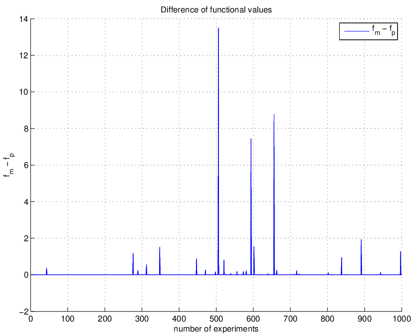
On one hand, each experiment was solved using Algorithm 6 and, on the other hand, it was considered as a nonlinear programming problem and solved using function (see [32] and references therein). Since the Weber function (1) is not differentiable at the vertices, nonlinear programming solvers may fail.
Let be the solution of (5) obtained by in experiment , and . Analogously, let be the solution of (5) obtained by Algorithm 6 in experiment , and . Figure 2 shows the difference between the arrays and . Both methods finished succesfully in all cases, however, Algorithm 6 found equal or better results for all experiments. For example, the difference was greater than in experiments (the maximum difference ocurred in experiment ).

7 Conclusions
This paper proposes a Weiszfeld-like algorithm for solving the Weber problem constrained to a closed and convex set, and it is well defined even when an iterate is a vertex. The algorithm consists of two stages: first, iterate using the fixed point modified Weiszfeld iteration (13), and second, either project onto the set when the iterate is different from the vertices, or, if the iterate is a vertex , take the point belonging to the line that joins with as defined in (14).
It is proved that the constrained problem (5) has a unique solution. Besides that, the definition of the iteration function allows us to demonstrate that the proposed algorithm produces a sequence of feasible iterates. Moreover, the sequence is not increasing, and when , the sequence decreases at the next iterate. It can be seen that if a point is the solution of the problem (5) then is a fixed point of the iteration function . Even more, if is different from the vertices, the fact of being a fixed point of is equivalent to the fact that satisfies the KKT optimality conditions, and equivalent to the fact that is the solution of the problem (5). These properties allows us to connect the proposed algorithm with the minimization problem.
Numerical experiments showed that the proposed algorithm found equal or better solutions than a well-known standard solver, in a practical example with 1000 random choices of vertices and weights. That is due to the fact that the proposed algorithm does not use of the existence of derivatives at the vertices, because the Weber function is not differentiable at the vertices.
References
- [1] N. Andréasson, A. Evgrafov, M. Patriksson, An introduction to continuous optimization, Studentlitteratur, 2007.
- [2] Y.P. Aneja, M. Parlar, Technical note-Algorithms for Weber facility location in the presence of forbidden regions and/or barriers to travel, Transportation Science 28 (1994) 70–76.
- [3] R.J. Cañavate Bernal, Algunas cuestiones teóricas sobre la validez del algoritmo de Weiszfeld para el problema de Weber, Rect@ Actas_13 (2005) 24.
- [4] M. Bischoff, T. Fleischmann, K. Klamroth, The multi-facility location-allocation problem with polyhedral barriers, Comput. Oper. Res. 36 (2009) 1376–1392.
- [5] M. Bischoff, K. Klamroth, An efficient solution method for Weber problems with barriers based on genetic algorithms, European J. Oper. Res. 177 (2007) 22–41.
- [6] J. Brimberg, The Fermat-Weber location problem revisited, Mathematical Programming 71 (1995) 71–76.
- [7] J. Brimberg, Further notes on convergence of the Weiszfeld algorithm, Yugosl. J. Oper. Res. 13 (2003) 199–206.
- [8] S.E. Butt, T.M. Cavalier, An efficient algorithm for facility location in the presence of forbidden regions, European J. Oper. Res. 90 (1996) 56–70.
- [9] L. Cánovas, R. Cañavate, A. Marín, On the convergence of the Weiszfeld algorithm, Mathematical Programming 93 (2002) 327–330.
- [10] E. Carrizosa, M. Muñoz-Márquez, J. Puerto, The Weber problem with regional demand, European J. Oper. Res. 104 (1998) 358–365.
- [11] R. Chandrasekaran, A. Tamir, Open questions concerning Weiszfeld’s algorithm for the Fermat-Weber location problem, Mathematical Programming 44 (1989) 293–295.
- [12] J.A. Chatelon, D.W. Hearn, T.J. Lowe, A subgradient algorithm for certain minimax and minisum problems, Mathematical Programming 15 (1978) 130–145.
- [13] P.C. Chen, P. Hansen, B. Jaumard, H. Tuy, Weber’s problem with attraction and repulsion, Journal of Regional Science 32 (1992) 467–486.
- [14] R. Courant, D. Hilbert, Methoden der mathematischen Physik. I, Springer-Verlag, Berlin, 1968. Dritte Auflage, Heidelberger Taschenbucher, Band 30.
- [15] Z. Drezner, On the convergence of the generalized Weiszfeld algorithm, Ann. Oper. Res. 167 (2009) 327–336.
- [16] Z. Drezner, G.O. Wesolowsky, The location of an obnoxious facility with rectangular distances, Journal of Regional Science 23 (1983) 241–248.
- [17] Z. Drezner, G.O. Wesolowsky, Sensitivity analysis to the value of of the distance Weber problem, Ann. Oper. Res. 111 (2002) 135–150.
- [18] U. Eckhardt, Weber’s problem and Weiszfeld’s algorithm in general spaces, Mathematical Programming 18 (1980) 186–196.
- [19] J.W. Eyster, J.A. White, W.W. Wierwille, On solving multifacility location problems using a hyperboloid approximation procedure, A I I E Transactions 5 (1973) 01–06.
- [20] E. Fasbender, Über die gleichseitigen Dreiecke, welche um ein gegebenes Dreieck gelegt werden können, Journal für die reine und angewandte Mathematik 30 (1846) 230–231.
- [21] P. Hansen, D. Peeters, J. Thisse, An algorithm for a constrained Weber problem, Management Science (1982) 1285–1295.
- [22] J. Jahn, Introduction to the theory of nonlinear optimization, Springer Verlag, 2007.
- [23] G. Jalal, J. Krarup, Geometrical solution to the Fermat problem with arbitrary weights, Ann. Oper. Res. 123 (2003) 67–104.
- [24] W. Kaplan, W. Yang, Duality theorem for a generalized Fermat-Weber problem, Mathematical Programming 76 (1997) 285–297.
- [25] I.N. Katz, L. Cooper, Facility location in the presence of forbidden regions. I. Formulation and the case of Euclidean distance with one forbidden circle, European J. Oper. Res. 6 (1981) 166–173.
- [26] K. Klamroth, Single-facility location problems with barriers, Springer Series in Operations Research, Springer-Verlag, New York, 2002.
- [27] J. Krarup, S. Vajda, On Torricelli’s geometrical solution to a problem of Fermat, IMA J. Math. Appl. Bus. Indust. 8 (1997) 215–224. Duality in practice.
- [28] H.W. Kuhn, On a pair of dual nonlinear programs, in: Nonlinear Programming (NATO Summer School, Menton, 1964), North-Holland, Amsterdam, 1967, pp. 37–54.
- [29] H.W. Kuhn, A note on Fermat’s problem, Mathematical Programming 4 (1973) 98–107.
- [30] Y.S. Kupitz, H. Martini, Geometric aspects of the generalized Fermat-Torricelli problem, in: Intuitive geometry (Budapest, 1995), volume 6 of Bolyai Soc. Math. Stud., János Bolyai Math. Soc., Budapest, 1997, pp. 55–127.
- [31] D.G. Luenberger, Y. Ye, Linear and nonlinear programming, International Series in Operations Research & Management Science, 116, Springer, New York, third edition, 2008.
- [32] MATLAB, http://www.mathworks.com/help/toolbox/optim/ug/fmincon.html, 2012.
- [33] C. Michelot, O. Lefebvre, A primal-dual algorithm for the Fermat-Weber problem involving mixed gauges, Mathematical Programming 39 (1987) 319–335.
- [34] M.L. Overton, A quadratically convergent method for minimizing a sum of Euclidean norms, Mathematical Programming 27 (1983) 34–63.
- [35] B. Pfeiffer, K. Klamroth, A unified model for Weber problems with continuous and network distances, Comput. Oper. Res. 35 (2008) 312–326.
- [36] E.A. Pilotta, G.A. Torres, A projected Weiszfeld algorithm for the box-constrained Weber location problem, Applied Mathematics and Computation 218 (2011) 2932–2943.
- [37] G. Polya, Mathematik und plausibles Schließen, Band 1, Induktion Und Analogie in Der Mathematik, Birkhauser, Basel, 1962.
- [38] A. Quarteroni, R. Sacco, F. Saleri, Numerical mathematics, volume 37, Springer, 2006.
- [39] M.K. Schaefer, A.P.J. Hurter, An algorithm for the solution of a location problem with metric constraints, Naval Res. Logist. Quart. 21 (1974) 625–636.
- [40] Y. Vardi, C.H. Zhang, A modified Weiszfeld algorithm for the Fermat-Weber location problem, Mathematical Programming 90 (2001) 559–566.
- [41] A. Weber, Über den Standort der Industrien, University of Chicago Press, Chicago, 1929. Translated by C. J. Friederich: “Theory of the location of industries”.
- [42] E. Weiszfeld, Sur le point par lequel la somme des distances de points donnés est minimum, Tohoku Mathematics Journal 43 (1937) 355–386.
- [43] E. Weiszfeld, On the point for which the sum of the distances to given points is minimum, Ann. Oper. Res. 167 (2009) 7–41.
- [44] G.O. Wesolowsky, The Weber problem: history and perspectives, Location Sci. 1 (1993) 5–23.