The relative and absolute timing accuracy of the EPIC-pn camera on XMM-Newton, from X-ray pulsations of the Crab and other pulsars
Abstract
Aims. Reliable timing calibration is essential for the accurate comparison of XMM-Newton light curves with those from other observatories, to ultimately use them to derive precise physical quantities. The XMM-Newton timing calibration is based on pulsar analysis. However, as pulsars show both timing noise and glitches, it is essential to monitor these calibration sources regularly. To this end, the XMM-Newton observatory performs observations twice a year of the Crab pulsar to monitor the absolute timing accuracy of the EPIC-pn camera in the fast Timing and Burst modes. We present the results of this monitoring campaign, comparing XMM-Newton data from the Crab pulsar (PSR B0531+21) with radio measurements. In addition, we use five pulsars (PSR J0537-69, PSR B0540-69, PSR B0833-45, PSR B1509-58 and PSR B1055-52) with periods ranging from 16 ms to 197 ms to verify the relative timing accuracy.
Methods. We analysed 38 XMM-Newton observations (0.2-12.0 keV) of the Crab taken over the first ten years of the mission and 13 observations from the five complementary pulsars. All the data were processed with the SAS, the XMM-Newton Scientific Analysis Software, version 9.0. Epoch folding techniques coupled with tests were used to derive relative timing accuracies. The absolute timing accuracy was determined using the Crab data and comparing the time shift between the main X-ray and radio peaks in the phase folded light curves.
Results. The relative timing accuracy of XMM-Newton is found to be better than . The strongest X-ray pulse peak precedes the corresponding radio peak by 3069 s, which is in agreement with other high energy observatories such as Chandra, INTEGRAL and RXTE. The derived absolute timing accuracy from our analysis is 48 s.
Key Words.
stars: neutron stars – pulsars: individual: PSR B0531+21, PSR J0537-69, PSR B0540-69, PSR B0833-45, PSR B1509-58, PSR B1055-52 – supernova remnants: Crab – X-rays: stars – instruments: EPIC-pn – data analysis: relative timing, absolute timing1 Introduction
A reliable timing calibration is essential for all timing data analyses and the physics derived from those. Irregularities in the spacecraft time correlation, the on-board instrument oscillators or data handling unit and the ground processing and data analysis software can lead to errors in relative and absolute information pertaining to the timing behaviour of astrophysical objects. The timing of the XMM-Newton observatory is evaluated using XMM-Newton’s EPIC-pn camera that has been extensively ground calibrated with respect to relative timing, but due to a limited calibration time budget, the end-to-end system for absolute timing was never checked on the ground. The relative timing for fast sources like the Crab was expected to have an accuracy of before launch. For the absolute timing a requirement of was given.
XMM-Newton (Jansen et al., 2001) was launched in December 1999 with an Ariane 5 rocket from French Guayana. It operates six instruments in parallel on its 48 hour highly elliptical orbit: three Wolter type 1 telescopes, with 58 nested mirror shells each, focus X-ray photons onto the three X-ray instruments of the EPIC (European Photon Imaging Camera) (Strüder et al., 2001; Turner et al., 2001) and the two Reflecting Grating Spectrometers (den Herder et al., 2001, RGS;). In addition, a 30 cm Ritchey Chrétien optical telescope, the Optical Monitor, is used for optical observations (Mason et al., 2001, OM;). EPIC consists of three cameras: the two EPIC-MOS cameras use Metal-Oxide Semiconductor CCDs as X-ray detectors, while the EPIC-pn camera is equipped with a pn-CCD. All three have been especially developed for XMM-Newton (Pfeffermann et al., 1999; Meidinger et al., 1999; Turner et al., 2001).
In this paper we determine the relative timing accuracy of XMM-Newton’s EPIC-pn camera using all available observations of the Crab pulsar in combination with other isolated pulsars in order to extend our analysis to a broader variety of sources. Preliminary results on the relative timing accuracy of XMM-Newton using the Crab pulsar and the other pulsars can be found in Caballero et al. (2006).
In this work we use only the Crab pulsar X-ray observations to determine the absolute timing accuracy. However, as this is done in reference to radio timing, it is limited to the accuracy of the radio ephemerides.
We also see the paper as a summary of "how to perform" relative and absolute timing analysis with XMM-Newton and what timing accuracy the user can expect for different targets.
This paper is organised as follows. In Sect. 2 we give a description of the targets used for the timing evaluation, followed by some technical comments on our data analysis in Sect. 3. The relative and absolute timing results are presented in Sect. 4 and Sect. 5. A short description of the XMM-Newton’s EPIC-pn camera is given in Appendix A.
2 Observations
All pulsars used in our analysis are isolated. We concentrated primarily on the Crab pulsar (PSR B0531+21) as radio ephemerides are provided monthly by the Jodrell Bank Observatory11 1 http://www.jb.man.ac.uk (Lyne et al., 1993). The other pulsars have been chosen to include a range of periods and pulse profiles, with which to check the relative timing. Some of these pulsar observations were reported by Becker et al. (2002) as a summary of first results from XMM-Newton.
Tables 1 and 2 summarise the data used and the results obtained from all the Crab observations studied and all the other pulsars respectively. Column 1 gives the observation ID (OBSID) used for identifying XMM-Newton observations, followed by the satellite revolution ("Rev.") in which the observation was done, the data mode, and the filter used. Column 5 indicates whether the observation is affected by telemetry gaps (due to a full science buffer), and column 6 gives information on time jumps during the observation (see the footnote of the table for explanation). Column 7 lists the start times ("Epoch") of the observations in MJD, followed by the exposure ("Obs. Time") in ks. Columns 9 and 10 list the pulse periods of the Crab pulsar in the radio at the time of the XMM-Newton observations (interpolated using the information provided by the Jodrell Bank Observatory) and the measured X-ray period, respectively. Red. (column 11) gives the reduced values found at the maximum of the respective distribution of the period search (the number of degrees of freedom, dof, was always 100 for the Crab pulsar), and "FWHM" is the full width at half maximum of the distribution. P/P is the relative difference between the radio and the X-ray period (Eq. 1 in Sect. 3.1). The "Phase Shift" (last column) shows the measured time shift of the main peak in the pulse profile between the X-ray and radio profiles, as explained in Sect. 3.2. All uncertainties given are at the 1 (68%) level. The ephemerides of all the targets used in the analysis are shown in Table 4. Fig. 1 shows the pulse profiles for all the pulsars analysed in this paper.
2.1 The main XMM-Newton timing monitoring source: PSR B0531+21 (The Crab pulsar)
Since the discovery of the Crab Pulsar (Staelin & Reifenstein, 1968), the Crab has been one of the best studied objects in the sky and it remains one of the brightest X-ray sources regularly observed. As a standard candle for instrument calibration, the 33 ms Crab pulsar has been repeatedly studied (monitored) by many astronomy missions in almost every energy band of the electromagnetic spectrum. However, recent analysis presented by Wilson-Hodge et al. (2011) showed that the flux of the Crab is not constant on long timescales at high energies. These flux variations seem to be related to the nebula and correspond to a flux drop of 7 % (70 mCrab) over two years (2008-2010). This might affect the status of the Crab as a standard candle in the future.
In the X-ray regime its pulse profile exhibits a double peaked structure with a phase separation of 0.4 between the first (main) and the second peak. X-ray emission at all phases, including the pulse minimum, was discovered by Tennant et al. (2001) using the Chandra observatory. Measurements of X-ray to radio delays between the arrival times of the main pulse in each energy range of the Crab pulsar have been reported using all high-energy instruments aboard INTEGRAL (Kuiper et al., 2003) and RXTE (Rots et al., 2004). The time delays were determined to be 28040 s and 34440 s respectively.
The Crab pulsar has been observed bianually to monitor the timing capabilities of XMM-Newton. Over the years an observation strategy has been established that makes very efficient use of the limited calibration time budget. XMM-Newton generally observed the Crab pulsar three times per orbit for 5 ks: at the beginning, in the middle, and the end of that orbit. These campaigns were carried out in spring and autumn when XMM-Newton has a different location in its orbit with respect to the Sun-Earth system. This guarantees the monitoring of the dependency of the timing with respect to XMM-Newton’s orbital position. Eventual irregularities in relative timing with respect to the orbital position could then be identified. A total of 38 observations with exposure times between 2 ks and 40 ks have been analysed in this paper. See Table 1 for details of these observations.
2.2 Other useful pulsars for relative timing analysis
2.2.1 PSR J0537-69
PSR J0537-69 is a young pulsar, about 5000 years in age, located in the Large Magellanic Cloud. It is embedded in the supernova remnant N157B and is considered to be the oldest known Crab-like pulsar. It is a very fast-spinning pulsar with a period of 16 ms, discovered by Marshall et al. (1998) using RXTE. No significant radio signal above a 5 threshold has been detected from the pulsar (Crawford et al., 2005). In the X-ray energy range, RXTE has monitored PSR J0537-69 for seven years (Marshall et al., 2004; Middleditch et al., 2006), providing a complete study of the behaviour of the pulsar. Middleditch et al. (2006) reported 23 sudden increases in frequency, called glitches and present in most of young pulsars. Due to this highly irregular activity (a glitch every 4 months) a contemporaneous ephemeris is important. Its pulse profile in the X-ray regime is characterized by a single narrow peak.
See Table 2 for details of the observations. Our 36 ks observation coincides with the RXTE monitoring campaign presented by Middleditch et al. (2006) and a good ephemeris was therefore guaranteed.
2.2.2 PSR B0540-69
This young pulsar (1500 years) was discovered in soft X-rays by Seward et al. (1984) with a period of 51 ms, in the field of the Large Magellanic Cloud and it is considered to be a Crab-like pulsar. Its pulse shape does not appear to change significantly from optical to hard X-rays (de Plaa et al., 2003). The pulsed radio emission was discovered in late 1989 appearing as a faint source (Manchester et al., 1993) and presenting a complex profile, very different from the simple sinusoidal one seen in X-rays (Fig.1). A glitch was reported by Zhang et al. (2001) before the XMM-Newton observations and confirmed by Livingstone et al. (2005b) using a 7.6 year RXTE campaign. The glitch activity of PSR B0540-69 is known to be less than that of the Crab pulsar (Livingstone et al., 2005b) but the presence of considerable timing noise was reported by Cusumano et al. (2003) using ASCA, BeppoSAX and RXTE observations made over a time interval of about 8 years. Therefore, despite the low glitch activity, long extrapolations of the ephemeris might not be reliable. See Table 2 for details of the observations.
2.2.3 PSR B0833-45 (Vela pulsar)
The Vela pulsar with a period of 89 ms was discovered by Large, Vaughan & Mills (1968) and it is associated with a supernova remnant. It is, with the Crab pulsar, one of the most active young/middle-age pulsars known, showing regular glitches. These glitches have been intensively studied for the Vela pulsar, where a dozen events in different energy ranges have been recorded and analysed over the past three decades (Helfand et al., 2001; Dodson et al., 2007). Due to these important irregularities close radio ephemerides are needed.
No Vela timing mode observations have been performed with XMM-Newton, but since the period is 89 ms the data in Small Window mode (time resolution of 5.7 ms) can be used for our purposes. Thus we have analysed the four observations listed in Table 2.
2.2.4 PSR B1509-58
This young pulsar (1700 years) is one of the most energetic pulsars known and has a pulse period of 151 ms. It is associated with the supernova remnant G320.4-1.2 and it has been well studied in all wavelengths since it was discovered in the soft X-ray band using Einstein (Seward et al., 1982). The pulse profile in X-rays of appears to be much broader than in radio, changing from a narrow peak shape into a more sinusoidal shape at high energies. Monitored by RXTE since its launch, and covering a 21 year time interval and in conjunction with radio data from the MOST and Parkes observatories, a detailed timing study has been carried out (Livingstone et al., 2005a), but no glitch was found in the entire data sample. This result makes PSR B1509-58 probably the only known young pulsar that does not present any glitches over long periods of time. This property means that it is well adapted to extrapolation over long time intervals and useful for absolute timing analyses (Rots et al., 1998). See Table 2 for details of the observations.
2.2.5 PSR B1055-52
PSR B1055-52, one of the Three Musketeers together with PSR B0656+14 and Geminga, is a middle-aged pulsar with a period of 197 ms. It was discovered by Vaughan & Large (1972) but it was only in 1983 that X-ray emission was first detected by Cheng & Helfand (1983) using the Einstein Observatory. Ögelman & Finley (1993) detected sinusoidal pulsations in X-rays up to 2.4 keV. More recently, De Luca et al. (2005) showed using XMM-Newton data that the pulsed emission is detectable up to 6 keV. Most middle-aged pulsars like PSR B1055-52 show reduced timing noise and fewer glitches compared to younger ones. See Table 2 for details of the observations. Results concerning these data have been originally published by De Luca et al. (2005).

| OBSID | Rev. | Mode | Filter | Counting mode | Time Jump | Epoch | Obs. Time | Radio period | X-ray period | Red. | FWHM | P/P | Phase Shift |
|---|---|---|---|---|---|---|---|---|---|---|---|---|---|
| [MJD] | [ks] | [ms] | [ms] | [s] | |||||||||
| 0122330801 | 56 | TI | T | NO | S | 51632.83 | 22.58 | 33.5083819072 | 33.5083817(1) | 433 | 1.37 | -0.60.4 | -1482 |
| 0135730701 | 234 | B | T | NO | N | 51988.64 | 10.00 | 33.5213091402 | 33.5213091(5) | 197 | 3.24 | 0.020.9 | -3374 |
| 0153750201 | 411 | B | M | YES | N | 52340.68 | 4.63 | 33.5341004722 | 33.5341001(7) | 79 | 6.78 | -0.92 | -2874 |
| 0153750301 | 411 | B | M | YES | N | 52341.29 | 9.00 | 33.5341224876 | 33.5341223(9) | 143 | 3.52 | -0.31 | -2964 |
| 0153750401 | 411 | TI | T | YES | N | 52341.42 | 9.00 | 33.5341272691 | 33.5341278(9) | 269 | 3.57 | 21 | -2172 |
| 0153750501 | 411 | B | M | YES | N | 52341.84 | 9.00 | 33.5341426021 | 33.5341426(5) | 136 | 3.55 | 0.21 | -2574 |
| 0160960201 | 698 | TI | T | YES | N | 52913.51 | 28.26 | 33.5549129334 | 33.5549128(4) | 912 | 1.58 | -0.30.5 | -1742 |
| 0160960301 | 700 | TI | T | YES | N | 52918.30 | 10.17 | 33.5550871157 | 33.5550881(2) | 313 | 4.58 | 31 | -2923 |
| 0160960401 | 874 | B | T | NO | N | 53264.10 | 14.72 | 33.5676516600 | 33.5676516(5) | 250 | 2.20 | -0.040.7 | 6033 |
| 0160960601 | 874 | B | T | NO | N | 53265.57 | 3.98 | 33.5677052394 | 33.5677050(1) | 68 | 8.01 | -0.72 | 88395 |
| 0160960701 | 955 | B | T | YES | N | 53425.72 | 8.20 | 33.5735256348 | 33.5735259(2) | 133 | 3.86 | 0.91 | -3343 |
| 0160960801 | 955 | B | T | YES | N | 53426.27 | 5.00 | 33.5735454128 | 33.5735452(4) | 80 | 6.52 | -0.52 | -3365 |
| 0160960901 | 955 | B | T | YES | N | 53426.77 | 8.20 | 33.5735638700 | 33.5735642(0) | 127 | 3.90 | 11 | -3574 |
| 0160961001 | 1048 | TI | T | YES | N | 53612.63 | 4.99 | 33.5803179048 | 33.580317(7) | 178 | 11.18 | -0.63 | -2573 |
| 0160961101 | 1049 | B | T | YES | N | 53613.14 | 5.00 | 33.5803366674 | 33.5803368(8) | 59 | 6.60 | 0.62 | -3354 |
| 0160961201 | 1049 | TI | T | YES | N | 53613.92 | 4.99 | 33.5803650194 | 33.580364(2) | 164 | 10.25 | -33 | -2862 |
| 0160961301 | 1140 | B | T | NO | N | 53794.72 | 5.00 | 33.5869348775 | 33.5869347(5) | 90 | 6.77 | -0.42 | -2844 |
| 0160961401 | 1140 | TI | T | YES | N | 53795.44 | 4.99 | 33.5869607624 | 33.5869607(3) | 262 | 6.18 | -0.12 | -2092 |
| 0160961501 | 1140 | B | T | NO | N | 53796.09 | 6.70 | 33.5869844395 | 33.5869844(8) | 129 | 4.47 | 0.11 | -3054 |
| 0312790101 | 1138 | B | T | YES | E | 53791.22 | 42.50 | 33.5868077617 | 33.5868078(5) | 422 | 1.25 | 0.30.4 | -2682 |
| 0312790201 | 1138 | B | T | NO | N | 53791.75 | 5.03 | 33.5868269683 | 33.5868267(9) | 72 | 6.46 | -0.52 | -3495 |
| 0312790401 | 1138 | B | T | NO | N | 53791.95 | 7.80 | 33.5868339621 | 33.5868344(5) | 52 | 4.19 | 11 | -3056 |
| 0412590101 | 1249 | B | T | NO | N | 54012.06 | 6.40 | 33.5948315461 | 33.5948316(2) | 111 | 4.82 | 0.21 | -3694 |
| 0412590201 | 1249 | TI | T | YES | N | 54012.72 | 5.04 | 33.5948556935 | 33.5948540(4) | 282 | 9.77 | -53 | -2842 |
| 0412590301 | 1249 | B | T | NO | N | 54013.38 | 8.85 | 33.5948794078 | 33.5948792(9) | 148 | 3.39 | -0.41 | -3893 |
| 0412590601 | 1325 | TI | T | YES | N | 54164.32 | 5.04 | 33.6003636968 | 33.6003640(7) | 241 | 6.14 | 12 | -5242 |
| 0412590701 | 1325 | B | T | YES | N | 54164.98 | 8.85 | 33.6003876860 | 33.6003877(0) | 156 | 3.50 | 0.031 | -6013 |
| 0412591001 | 1414 | B | T | NO | N | 54341.11 | 13.20 | 33.6067862758 | 33.6067861(8) | 220 | 2.33 | -0.30.7 | -3363 |
| 0412591101 | 1414 | TI | T | YES | N | 54341.96 | 5.00 | 33.6068170822 | 33.6068166(3) | 308 | 8.62 | -13 | -3033 |
| 0412591201 | 1414 | B | T | NO | S | 54342.40 | 13.41 | 33.6068330929 | 33.6068330(5) | 228 | 2.40 | -0.10.7 | -3603 |
| 0412591401 | 1504 | B | T | YES | N | 54520.72 | 21.70 | 33.6133108411 | 33.6133108(9) | 394 | 1.45 | 0.14 | -3572 |
| 0412591501 | 1504 | TI | T | YES | N | 54521.46 | 7.64 | 33.6133378231 | 33.6133377(7) | 521 | 4.53 | -0.11 | -2822 |
| 0412591601 | 1504 | B | T | YES | N | 54521.85 | 20.20 | 33.6133519405 | 33.6133519(9) | 382 | 1.51 | 0.10.4 | -3632 |
| 0412591901 | 1600 | B | T | YES | N | 54712.22 | 5.80 | 33.6202664839 | 33.6202667(5) | 133 | 5.50 | 0.82 | -2823 |
| 0412592001 | 1600 | TI | T | YES | N | 54712.78 | 6.04 | 33.6202865236 | 33.6202880(2) | 544 | 7.19 | 42 | -2072 |
| 0412592101 | 1600 | B | T | YES | N | 54713.35 | 15.39 | 33.6203076395 | 33.6203076(3) | 365 | 1.98 | -0.020.6 | -2632 |
| 0412592401 | 1687 | B | T | YES | N | 54885.70 | 18.90 | 33.6265670615 | 33.6265671(0) | 355 | 1.67 | 0.10.5 | -3792 |
| 0412592501 | 1687 | TI | T | YES | N | 54886.52 | 4.54 | 33.6265967322 | 33.6265966(8) | 341 | 6.78 | -0.12 | -3052 |
| Object | OBSID | Rev. | Mode | Filter | Epoch | Obs. Time | Reference period | Reference Epoch | X-ray period | Red. | FWHM | P/P |
|---|---|---|---|---|---|---|---|---|---|---|---|---|
| [MJD] | [ks] | [ms] | [MJD] | [ms] | ||||||||
| PSR J0537X | 0113020201 | 357 | TI | M | 52232.95 | 35.93 | 16.1229802136 | 52260.40296 | 16.1229802(3) | 24 | 0.38 | |
| PSR B0540X | 0125120201 | 85 | TI | M | 51691.54 | 17.05 | 50.5192855014 | 51686.20757 | 50.519284(6) | 99 | 12.60 | |
| PSR B0540R | 0125120201 | 85 | TI | M | 51691.54 | 17.05 | 50.5194431419 | 52857.86600 | 50.519284(6) | 99 | 12.60 | |
| PSR B0540X | 0413180201 | 1248 | TI | M | 54010.06 | 12.64 | 50.6160286612 | 52857.86600 | 50.615225(9) | 112 | 17.34 | |
| PSR B0540X | 0413180301 | 1248 | TI | M | 54010.79 | 15.24 | 50.6160594083 | 52857.86600 | 50.615252(7) | 136 | 14.75 | |
| VelaR | 0111080101 | 180 | SW | M | 51880.00 | 37.90 | 89.3318630836 | 52408.00000 | 89.331848(3) | 18 | 7.90 | |
| VelaR | 0111080201 | 180 | SW | M | 51880.51 | 58.60 | 89.3318685573 | 52408.00000 | 89.331853(2) | 25 | 6.01 | |
| VelaR | 0111080301 | 180 | SW | M | 51881.23 | 1.94 | 89.3318762404 | 52408.00000 | 89.33181(3) | 2 | 81.00 | |
| VelaR | 0153951401 | 1169 | SW | M | 53852.54 | 120.87 | 89.3531575271 | 53193.00000 | 89.352786(3) | 17 | 8.47 | |
| PSR B1509R | 0128120401 | 137 | TI | M | 51794.26 | 9.60 | 151.1145869352 | 50352.00000 | 151.11357(1) | 198 | 190.19 | |
| PSR B1509R | 0312590101 | 1136 | TI | M | 53786.98 | 31.95 | 151.3773132754 | 53385.00000 | 151.37723(1) | 694 | 58.35 | |
| PSR B1055R | 0113050101 | 186 | TI | M | 51892.93 | 19.90 | 197.1118094698 | 50256.00000 | 197.1118(1) | 30 | 151.09 | |
| PSR B1055R | 0113050201 | 187 | TI | M | 51893.73 | 52.70 | 197.1118098756 | 50256.00000 | 197.11183(5) | 34 | 65.81 |
3 Data analysis
The data sets were processed using the XMM-Newton Scientific Analysis Software, SAS 9.0 (Gabriel et al., 2004). Event times were corrected to the solar system barycentre using the SAS tool barycen.
3.1 Relative timing data analysis
We define the relative timing accuracy as the difference between the period measured with XMM-Newton and the period measured at radio wavelengths evaluated at the epoch of the X-ray observations. This difference is normalised to the pulse period measured in radio.
| (1) |
where
-
period derived from XMM-Newton
-
period extrapolated from radio ephemeris
-
time of the first X-ray event of the XMM-Newton observation [MJD]
We determined the period of the Crab pulsar in X-rays using the epoch folding software XRONOS44 4 XRONOS is part of the HEARSAC software (http://heasarc.gsfc.nasa.gov).. The closest available radio ephemeris (supplied by the Jodrell Bank Crab Pulsar Monthly Ephemeris) before and after the X-ray observation were used to interpolate the radio period P for the time of the first X-ray event of the XMM-Newton observation in MJD. The interpolated radio periods are then used as an initial trial value for the epoch folding. The period derivative provided by Jodrell Bank is taken into account when doing the folding of the X-ray data. All relevant initial and final values are listed in Tables 1, 2, 3 and 4. All X-ray pulse profiles shown in Fig. 1 have been produced using the best fit X-ray period.
The detailed steps of our data reduction are presented below in order to provide an example for proper XMM-Newton relative timing data analysis.
- 1.
calibrate the XMM-Newton event list using the SAS routine epproc55 5 command line set up of epproc: timing=YES burst=YES srcra=83.633216667 srcdec=22.014463889 withsrccoords=yes
- 2.
perform barycentre correction using precise coordinates with the SAS routine barycen66 6 command line set up of barycen: withtable=yes table=’bary.ds:EVENTS’ timecolumn=’TIME’ withsrccoordinates=yes srcra=’83.633216667’ srcdec=’22.014463889’ processgtis=yes time=0
- 3.
extract source77 7 Detector coordinates used in the extraction process a) timing mode: (RAWX,RAWY) IN box(35,101,12,100,0), b) burst mode: (RAWX,RAWY) IN box(35.,71.5,20,70,0)
- 4.
extrapolate the radio ephemeris
- 5.
period search using efsearch from XRONOS (see Table 3) which gives the against the period
- 6.
period determined through a weighted mean of all values within 65 of the efsearch maximum
| Object | nper | nphase | dres | Ṗ |
|---|---|---|---|---|
| PSR J0537 | 5000 | 15 | 5.1815 | |
| Crab | 5000 | 100 | 0.4205 | |
| PSR B0540 | 10000 | 20 | 4.78907 | |
| Vela | 2000 | 30 | 1.25008 | |
| PSR B1509 | 50000 | 50 | 1.53085 | |
| PSR B1055 | 40000 | 14 | 5.8354873 |
| Object | RA | Dec | epoch | |||
|---|---|---|---|---|---|---|
| (J2000) | (J2000) | [MJD] | [mHz] | [x10-10 Hz] | [x10-21 Hz] | |
| PSR J05371 | 05:37:47.20 | -69:10:23.00 | 52260.40296 | 62.02279999(0) | -1.993398(1) | 6.80(0) |
| Crab2 | 05:34:31.97 | 22:00:52.07 | – | – | – | – |
| PSR B05403 | 05:40:11.22 | -69:19:54.98 | 51686.20757 | 19.794507(5) | -1.881021(0) | 3.79(9) |
| PSR B05404 | 05:40:11.22 | -69:19:54.98 | 52857.86600 | 19.77552961(8) | -1.87288(3) | 4.30(2) |
| PSR B05404 | 05:40:11.22 | -69:19:54.98 | 52857.86600 | 19.775529611(3) | -1.872853(1) | 4.18(1) |
| Vela 5 | 08:35:20.61 | -45:10:34.87 | 52408.00000 | 11.193503640388(1) | -0.156027(3) | 0.64(1) |
| Vela6 | 08:35:20.61 | -45:10:34.87 | 53193.00000 | 11.192447207118304(3) | -0.155502(8) | 0.52(7) |
| PSR B15097 | 15:13:55.62 | -59:08:09.00 | 50352.00000 | 6.625918674074(4) | -0.673579(0) | 1.95(0) |
| PSR B15098 | 15:13:55.62 | -59:08:09.00 | 53385.00000 | 6.608333867737907(3) | -0.66852(2) | 1.91(4) |
| PSR B10559 | 10:57:58.84 | -52:26:56.30 | 50256.00000 | 5.073283989285(9) | -0.015019(5) | 3.24(0) |
The number of phase bins per period (nphase) in each pulse profile was chosen such that the count rate uncertainties in each bin (determined using the Poisson error on the count rate per bin normalised by the bin size) are, on average, not bigger than approximately 10% of the total count rate variation in the pulse profile of the shortest observation for each pulsar. This value, determined for each pulsar, is used for all the observations of that object. In this way the signal to noise in each bin is sufficient to reliably determine any ’smearing out’ of the pulse profile due to the use of an inaccurate period/ephemeris, essential for determining the relative timing precision, as described in Sect. 4.
3.2 Absolute timing data analysis
The XMM-Newton EPIC-pn absolute timing accuracy was determined using only observations of the Crab. The ephemeris (epoch, P, , ) of the nearest radio observation from the Jodrell Bank Observatory was used as a reference to obtain the phase shift between the time of arrival of the main peak in the X-ray profile and the time of arrival of the main peak in the radio profile, as described in Eq. 2. The phase shift was then multiplied by the corresponding X-ray period found during the relative timing analysis, as shown in Table 1.
| (2) |
where
-
Time of arrival of the main peak of the X-ray profile
-
Time of arrival of the main peak of the radio profile
The phase of the main X-ray peak was determined using a pulse profile with 1000 phase bins which was then fitted with an asymmetrical Moffat function. The explicit formula for the Moffat function is given in Appendix C. We also demonstrate how its shape varies when different parameters are modified. Fig 2 shows an example of how the phase of one Crab X-ray pulse profile (obs. ID: 0122330801) is slightly shifted in phase with respect to the radio phase (shown as a red line).

The following steps describe an example of the data reduction carried out on the XMM-Newton data in order to assess the absolute timing precision:
-
Steps 1-3 are the same as described in Sect. 3.1
- 4
fold the X-ray data on the radio period
- 5
fit the X-ray pulse profile with a Moffat function
- 6
determine the shift between the radio phase zero and the X-ray peak.
3.3 Evaluating the efficiency of automatic corrections made to event time jumps by the SAS
In order to do proper timing analysis with the EPIC data, every event detected on board has to be assigned a correct photon arrival time. The transformation from readout sequences by the EPIC camera to photon arrival times of each photon is performed by the EPEA (European Photon Event Analyser, Kuster et al. 1999). The absolute timing adjustment from On Board Time to UTC is done with the XMM-Newton time correlation (Kirsch et al., 2004). A hardware problem in the EPEA can produce time jumps in some observations, which have to be corrected.
A time jump can affect the timing accuracy by broadening the -distribution during the epoch folding search or by producing ’ghost peaks’ (Kirsch et al., 2004).


To find time jumps reliably one needs to have as accurate CCD frame times as possible. The frame times for all EPIC-pn modes using all available archive data (Freyberg et al., 2005) were remeasured and cross-checked with an independent method, analysing the evolving differences between consecutive events. If these differences are correct, the slope of the relation between the difference between the arrival times of consecutive events and the same quantity modulo the frame time is zero. Fig. 3 shows the effect of the frame time recalibration, which brought the values of this slope very close to zero for all observational modes. Constant ’timediff’ values’ indicate constant frame time.
Recalibration of the time jump detection algorithm of the XMM-Newton SAS has been done with the refined frame times. A search for time jumps in all available XMM-Newton archive data up to revolution 1061 showed a significant number of time jumps in the data for each observational mode. The application of the new algorithm reduced the number of remaining time jumps significantly. The effects of the SAS_JUMP_TOLERANCE parameter in the new algorithm (Versions 2-7) are shown in Fig. 4 for each EPIC-pn mode. The Version 0 shown in Fig. 4 represents the remaining time jumps with the old frame times and the old algorithm and it is included for comparison. Version 1 was obtained using the new frame times but with the old algorithm. While the rate of non-corrected time jumps (averaged over all pn-modes) was 2.8 per 100 ks before the implementation of the SASv8.0 time jump correction, just 0.3 time jumps per 100 ks remained uncorrected after its implementation. A breakdown of time jumps for each EPIC-pn mode is given in Table 5. This new improved algorithm has been implemented in the SAS as the default setting since version 8.0 (SAS_JUMP_TOLERANCE = 22.0). Table 1 indicates for which Crab observation a time jump has been corrected, and where data had to be excluded from the analysis.
In order to identify possible remaining time jumps, the data can be processed without the "fine-time"-correction, i.e., epframes set="infile_pn" eventset=events.dat gtiset=tmp_g.dat withfinetime=N. Then the time t between successive events is calculated and divided by the frame time, FT, of the relevant mode (FF Mode: 73.36496 ms, eFF Mode: 199.19408 ms, LW mode: 47.66384 ms, SW Mode: 5.67184 ms, Timing Mode: 5.96464 ms, Burst Mode: 4.34448 ms).
A time jump is shown to exist when t/FT is different from an integer by a quantity larger than a tolerance parameter. Only those time jumps which happen to be an integer multiple of the relevant FT would not be found with this method. It is important to notice that the tolerance acceptable between t and the full frame time should not be bigger than (20/48828.125FT).
| pn instrument mode | Pre SASv8.0 | Post SASv8.0 |
|---|---|---|
| per 100 ks | per 100 ks | |
| Full Frame (FF) | 0.6 | 0.2 |
| Extended Full Frame (eFF) | 2.1 | 0.2 |
| Small Window (SW) | 3.7 | 0.7 |
| Large Window (LW) | 3.9 | 0.1 |
| Timing | 1.2 | 0.1 |
| Burst | 5.3 | 0.3 |
| Overall mean | 2.8 | 0.3 |

4 Relative Timing accuracy of XMM-Newton
The relative timing accuracy of the EPIC-pn camera has been studied using all six pulsars (see Fig. 1), presented in Sect. 2.
As described in Appendix B, the FWHM of the curve obtained during the period search analysis can be expressed in terms of the period and the exposure time of the observation (Eq. 6). From this expression, and using the Independent Fourier Space (de Oña Wilhelmi, 2003, IFS;), approach discussed in the appendix, an empirical formula for the error on the X-ray period was found (Eq. 3).
| (3) |
where dof is the number of degrees of freedom (number of phase bins used to construct the pulse profiles minus the number of variables). The number of bins used in the pulse profiles are shown in Table 3.
The relative timing accuracy was defined by Eq. 1 and therefore its error will depend mostly on how accurately the radio and X-ray periods can be measured. Other factors that could affect the relative timing accuracy are discussed in Appendix B. Considering that the radio period measurements are more accurate than the X-ray periods (usually by 1-3 orders of magnitude; however, DM variations can sometimes cause problems and the time resolution of the radio telescopes has to be monitored), it was assumed in our analysis that their errors were negligible compared to the error on the X-ray period. Thus, it can be found that the relative timing, P depends exclusively on the error of the X-ray period, P as shown in Eq. 4.
| (4) |
The relationship described in Eq. 4 allows a goodness of fit study of our measured P compared to the empirical P described in Eq. 3. The empirical P was considered as an upper limit on an accurate P measurement. A comparison between the observed relative timing accuracy in absolute value and normalised by the corresponding period, P/P (symbols) and its “expected” value obtained from Eq. 3 and Eq. 4 (lines) is presented in Fig. 5 as a function of the exposure time and in Fig. 6 as a function of date.

For observations where we have very reliable radio/X-ray ephemerides, the observed data points are below the lines of the estimated accuracies. The outliers above the respective theoretical lines for each individual pulsar are described below:
- 1.
Radio ephemerides extrapolated over long time intervals appear to be unreliable. Therefore, we exclude the following observations in the final calculation regarding the relative timing accuracy: Vela pulsar: 015395140; PSR B1509-58: 0128120401; PSR B0540-69: 0413180201, 0413180301.
- 2.
The P approximation given in Eq. 4 was found to be unreliable in some cases (e.g. for PSR B1509-58, observation: 0312590101 and the Vela pulsar, observations: 0111080101, 0111080201). As the Vela pulsar is quite active, we may have under-estimated the error by simply extrapolating the ephemeris, however, the same can not be said about PSR B1509-58 which is one of the most stable young pulsars known.
As seen in Fig. 6 there is no obvious change in the relative timing accuracy of the EPIC-pn camera over its lifetime.

The results for the Crab pulsar alone are shown in Fig. 7. As expected, there is a tendency towards smaller uncertainties for longer observations.
For a quantitative measure of the timing accuracy the standard deviation for the P/P distribution (shown in Fig. 6) was used. Fitting the distributions with a Gaussian normal distribution, we found a standard deviation of for all the pulsars together (including the Crab pulsar) and for the Crab pulsar alone. While the distribution for Crab pulsar is centred at zero (within uncertainties) the mean value of the distribution for all the pulsars combined is slightly offset, in the sense that the X-ray period is slightly shorter on average than the radio period. Thus, the relative deviation of the observed pulse period with respect to the most accurate radio data available is P/P .


5 Absolute timing accuracy of XMM-Newton
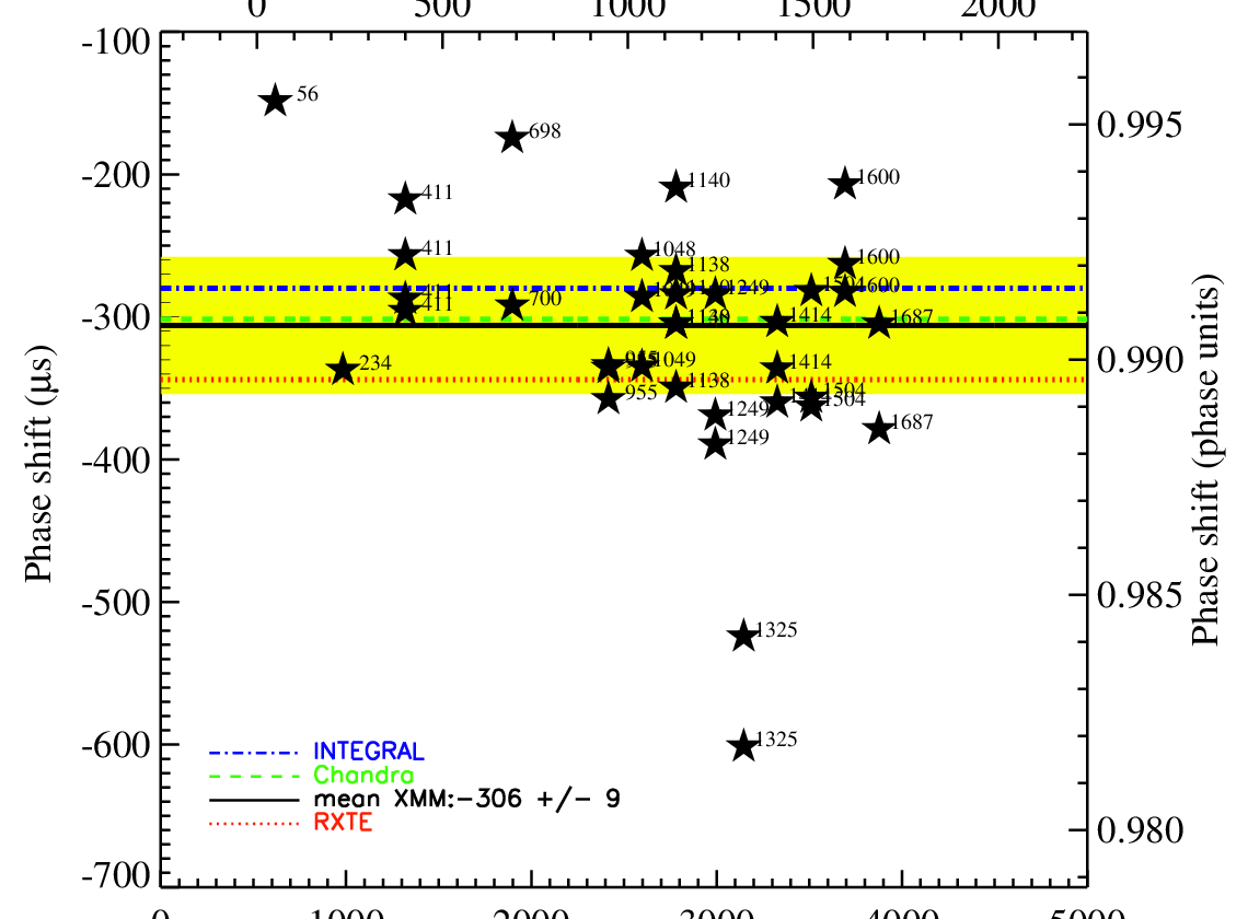
The Crab pulsar shows a shift of -306 s (shown in Fig. 8) between the peak of the first X-ray pulse with respect to the radio peak. We hereby confirm the similar results of other missions like Chandra (Tennant et al., 2001), INTEGRAL (Kuiper et al., 2003), and RXTE (Rots et al., 2004). The XMM-Newton values ("stars" in Fig. 8) show a considerable scatter with a standard deviation of 48 s. The formal error on the mean value of -306 s is s.
The scatter found is consistent with the previously determined maximum integrated error for the time correlation of less than 100 s (Kirsch et al., 2005). The original requirement for an absolute timing accuracy of 1 ms for XMM-Newton, defined before launch, has clearly been reached and even improved on by at least a factor of 20.
This scatter is likely to be due to uncertainties in the time correlation process since the phase of the main peak can be measured with an accuracy of s. Upper limits for these processes were reported by Kirsch et al. (2004)1010 10 http://xmm2.esac.esa.int/docs/documents/CAL-TN-0045-1-0.pdf who gave a detailed description of all kinds of instrumental delays considered while converting between observing time and UTC time and estimated the spacecraft clock error to be 11 s, the uncertainty in ground station delays to be 5 s, the interpolation errors to be 10 s, the error between latching observing time and the start of frame transmission as 9 s, and the uncertainties in the spacecraft orbit ephemeris to be 30 s. All these errors will be random for our data, and hence the fluctuations observed. The 48 s 1 scatter measured with respect to the mean may then be attributed uniquely to the above errors and no other systematic effect. This value can then be considered to be the minimal significant time separation between two arrival times to be considered independent.
From the initial 38 Crab observations, 32 were considered for the absolute analysis. Six of the Crab observations were excluded for the reasons given below:
- •
Observation 0122330801: was early in the mission (rev. 56) and appears to have problems in the time correlation that can no longer be recovered.
- •
Observation 0160960201: too much data had to be excluded due to time jumps which caused a dramatic reduction in the number of counts (rev 698).
- •
Observations 0160960401 and 0160960601: these correspond to rev. 874 which shows the X-ray pulse peak displaced from the expected radio position. This is likely to have been caused by a glitch shortly before the XMM-Newton observations. This offset is more dramatic in the second observation, which has poorer statistics due to a shorter exposure time. None of these observations fall into the range shown in Fig. 8.
- •
Observations 0412590601 and 0412590701: these correspond to rev. 1325. The reason for the offsets is unclear. They may be due to a small, non-reported glitch or an anomalously large ground segment error, but because of the uncertainty, we excluded these observations when determining the absolute timing precision.
It was found that some observations presented pulse profiles with an excess of counts in the interpulse region of the Crab profile. Numerical simulations have been used to study the effect that this excess could have caused in determining the peak of the X-ray profile and thus, in determining the difference in phase between the X-ray and the radio. Using the typical 0.2-15.0 keV Crab profile as the input, 10000 light curves were created using Monte Carlo simulations. The strength of both peaks in the pulse profile (keeping the ratio between them constant) as well as the strength of the interpulse were selected as input parameters. As shown in Fig. 14 in Appendix C, the Moffat fit, used to determine the phase of the main peak, can be used to reliably fit different tails. To fit the excess in the interpulse we added a Lorentzian function to the pulse profile in order to take into account the excess in the tail of the main peak. The secondary peak was omitted in the fit. No phase shift was found in any of the models tried, which implies that the strength of the interpulse region plays no role in determining the phase of the peak of the profile and thus all 32 of the retained Crab observations could be used to derive the absolute timing accuracy reliably.
6 Discussion and Conclusion
The Crab pulsar has been used by many missions as a calibration source for timing accuracy (Kuiper et al. (2003), Rots et al. (2004), Oosterbroek et al. (2008), Abdo et al. (2010), Molkov et al. 2010). The XMM-Newton observatory began observing the Crab pulsar during its earliest orbits, monitoring its X-ray pulsation with high time resolution. 38 Crab observations spread over 10 years have been analysed in this paper (from revolution 56 until revolution 1687). Measurements of the period were made with an accuracy of 10-11 s. A relative timing accuracy smaller than 10-8 and stable with time was established for the EPIC-pn camera. This result was achieved by comparing our X-ray measurements of the Crab pulsar with high precision radio measurements at each corresponding epoch. Five isolated pulsars showing a wide range of periods and completely different pulse profiles (PSR J0537-69, PSR B0540-69, Vela pulsar, PSR B1509-58 and PSR B1055-52) were analysed to complement the study of the relative timing accuracy, confirming the results obtained with the Crab pulsar.
For the case of PSR B0540-69 a long term phase-coherent study of its period was reported by Livingstone et al. (2005b). Due to its stability we considered it a good candidate to use for an extrapolation over a long time period. As shown in Table 2 the long extrapolation made in two of the three observations of PSR B0540-69 show poor results suggesting that a small glitch between the ephemeris and our observation may have occurred, rendering this pulsar less stable than anticipated.
An improved algorithm to detect and correct sporadic "jumps” in the flow of the photon arrival times has been implemented with SASv8.0 (Guainazzi et al., 2011)1111 11 http://xmm2.esac.esa.int/docs/documents/CAL-TN-0018.pdf. This method is based on a more accurate determination of the frame times for all pn modes and on a correction of frame time drifts due to temperature variation and aging of the on-board clock (Freyberg et al., 2005). The total reduction of the rate per 100 ks of observation affected by residual uncorrected time jumps for all pn instrumental modes dropped from 2.8 before the improved algorithm to 0.3 once it was implemented.
For the absolute timing analysis, only Crab pulsar observations have been analysed since a high number of stable observations need to be considered to provide a reliable result. We have considered the phase of the first (main) peak of the X-ray profile and measured the phase difference with respect to the corresponding peak of the radio profile. Considering 32 of 38 Crab EPIC-pn observations (0.2-12 keV energy range) analysed in this paper, we confirmed previous results demonstrating that the first X-ray peak from the Crab pulsar leads the radio peak by 306 9 s (statistical error) with 48 s (1 ) scatter. This error is similar to the Ground Segment accuracy and defines the absolute timing accuracy of the instrument. The observed shift is consistent within 1 with those presented by Kuiper et al. (2003) using INTEGRAL and by Rots et al. (2004) using RXTE, as shown in Fig. 8.

A systematic comparison of our measurements in the X-ray band with respect to other accurate measurements carried out in different energy bands from earlier observations in the optical, X-ray, and -ray parts of the spectrum are shown in Fig. 9. Differences in the shifts observed over 7 decades in energy are marginal with an average value of 284.4 s. It is important to note that the large error bars quoted in the X-ray band for XMM-Newton and RXTE include systematic errors from the radio measurements, carried out at the Jodrell Bank Observatory.
The origin of the electromagnetic radiation emitted from pulsars is still unclear. Several models have been proposed to explain the origin of the high energy radiation based on different regions of acceleration in the pulsar magnetosphere, such as the polar cap, the slot gap and the outer gap models (Harding et al., 1978; Arons & Scharlemann, 1979; Cheng et al., 1986; Zhang & Harding, 2000; Harding & Muslimov, 2011, e.g.). The radio emission model is an empirical one and the radiation is usually assumed to come from a core beam centered on the magnetic axis and one or more hollow cones surrounding the core (Rankin, 1983, e.g.). The estimated average delay between the emission from differing wavelengths is therefore very significant. It implies that the site of radio production is distinctly different from that of the non-radio emission. The difference in phase between the radio and the X-ray radiation is about 0.008, or three degrees in phase angle. This time delay of about 300 s most naturally implies that emission regions differ in position by about 90 km between radio and X-rays energy bands in a simplistic geometrical model neglecting any relativistic effects, with the radio being emitted from closer to the surface of the neutron star. Such high time resolution, high precision absolute timing, multiwavelength observations are therefore essential for understanding the origin of the pulsar emission.
Acknowledgements.
The XMM-Newton project is an ESA Science Mission with instruments and contributions directly funded by ESA Member States and the USA (NASA). The German contribution of the XMM-Newton project is supported by the Bundesministerium für Bildung und Forschung/Deutsches Zentrum für Luft- und Raumfahrt. The UK involvement is funded by the Particle Physics and Astronomy Research Council (PPARC). The Parkes radio telescope is part of the Australia Telescope which is funded by the Commonwealth of Australia for operation as a National Facility managed by CSIRO. We wish to thank Dr. L. Kuiper for all his help on the absolute timing analysis procedure and results and all the discussions and comments that he provided to the development of this paper. We would also like to thank the anonymous referee for his/her useful comments and suggestions. A. Martin-Carrillo also wish to thank the ESAC Faculty group for their financial support during the investigation and creation of this publication.References
- Abdo et al. (2010) Abdo, A. A. et al. 2010, ApJ, 708, 1254
- Arons & Scharlemann (1979) Arons, J., & Scharlemann, E. T., 1979, ApJ, 231, 854
- Becker et al. (2002) Becker, W. & Aschenbach, B. Proc. of the 270. WE-Heraeus Seminar on: "Neutron Stars and Pulsars" , R. 278, pp. 64-86 (2002)
- Caballero et al. (2006) Caballero, I. et al. 2006, Proc. Conference "The X-ray Universe", Wilson, A. eds. 604, 963
- Cheng & Helfand (1983) Cheng, A. F., & Helfand, D. J. 1983, ApJ, 271, 271
- Cheng et al. (1986) Cheng, K. S., Ho, C., & Ruderman, M. 1986, ApJ, 300, 500
- Cusumano et al. (2003) Cusumano, G., et al. 2003, A&A, 402, 647
- Crawford et al. (2005) Crawford, F., et al. 2005, AdSpR, 35, 1181
- De Luca et al. (2005) De Luca, A. et al. 2005, ApJ, 623, 1051
- Dodson et al. (2007) Dodson, R., et al. 2007, Ap&SS, 308, 585
- Freyberg et al. (2005) Freyberg, M. J., Burkert, W., Hartner, G. ., Kirsch, M. G. F., & Kendziorra, E. . 2005, 5 years of Science with XMM-Newton, 159
- Gabriel et al. (2004) Gabriel, C. et al. 2004, ASPC, Vol. 314, 759
- Guainazzi et al. (2011) Guainazzi, M. et al. 2011, XMM-CAL-SOC-TN-0018
- Harding et al. (1978) Harding, A. K., Tademaru, E., & Esposito, L. W., 1978, ApJ, 225, 226
- Harding & Muslimov (2011) Harding, A. K., & Muslimov, A. G. 2011, ApJ, 726, L10
- Helfand et al. (2001) Helfand, D. J. et al., 2001, ApJ, 556, 380
- den Herder et al. (2001) den Herder, J. W., et al. 2001, A&A, 365, L7
- Jansen et al. (2001) Jansen, F., et al. 2001, A&A, 365, L1
- Johnston et al. (2004) Johnston, S. et al. 2004, MNRAS, 355, 31
- Kendziorra et al. (1999) Kendziorra, E., et al. 1999, EUV, X-Ray, and Gamma-Ray Instrumentation for Astronomy X, O. Siegmund & K. A. Flanagan eds., Proc. SPIE, 3765, 204
- Kirsch et al. (2004) Kirsch, M.G.F, et al. 2004, X-Ray and Gamma-Ray Instrumentation for Astronomy XIII. Edited by Flanagan, Kathryn A.; Siegmund, Oswald H. W. Proceedings of the SPIE, Volume 5165, 85-95
- Kirsch et al. (2005) Kirsch, M. G. F., et al. 2005, Proceedings of the SPIE, Volume 5898, 22-33
- Kirsch et al. (2006) Kirsch, M. G. F., et al. 2006, A&A, 453, 173
- Kuiper et al. (2002) Kuiper, L. et al. 2002, ApJ, 577, 917
- Kuiper et al. (2003) Kuiper, L. et al. 2003, A&A, 411, L31
- Kuster et al. (1999) Kuster, M., et al. 1999, EUV, X-Ray, and Gamma-Ray Instrumentation for Astronomy X, O. Siegmund & K. A. Flanagan eds., Proc. SPIE, 3765, 673
- Large, Vaughan & Mills (1968) Large, M. I., Vaughan, A. E. & Mills, B. Y., Nature, 220, L340
- Lyne et al. (1993) Lyne, A. G., Pritchard, R. S., Smith, F. G. 1993, MNRAS, 265, 1003
- Livingstone et al. (2005a) Livingstone, M. A. et al. 2005a, ApJ, 619, 1046
- Livingstone et al. (2005b) Livingstone, M. A. et al. 2005b, ApJ, 633, 1095
- Manchester et al. (1993) Manchester, R. N., Mar, D. P., Lyne, A. G., Kaspi, V. M., & Johnston, S. 1993, ApJ, 403, L29
- Marshall et al. (1998) Marshall. F. E. et al. 1998, ApJ, 499, L179
- Marshall et al. (2004) Marshall, F. E. et al. 2004, ApJ, 603, 682
- Mason et al. (2001) Mason, K.O., et al. 2001, A&A, 365, L36
- Massaro et al. (2000) Massaro, E., Cusumano, G., Litterio, M. & Mineo, T. 2000, A&A, 361, 695
- Meidinger et al. (1999) Meidinger, N. et al. 1999, EUV, X-Ray, and Gamma-Ray Instrumentation for Astronomy X, O. Siegmund and K. A. Flanagan eds., Proc. SPIE, 3765, 192
- Middleditch et al. (2006) Middleditch, J. et al. 2006, ApJ, 652, 1531
- Mineo et al. (2002) Mineo, T. et al. 2004, A&A, 392, 181
- Moffat (1969) Moffat, A.F.J. 1969, A&A, v. 3, p.455-461
- Molkov et al. (2010) Molkov, S. et al. 2010, ApJ, 708, 403
- Mori et al. (2004) Mori, K. et al. 2004, Advances in Space Research, 33, 503
- Mori et al. (2004) Mori, K., Burrows, D. N., Hester, J. J., Pavlov, G. G., Shibata, S., & Tsunemi, H. 2004, ApJ, 609, 186
- Ness et al. (2010) Ness, J., U., et al. 2010, XMM-Newton Users Handbook, Issue 2.8.1
- Ögelman & Finley (1993) Ögelman, H., & Finley, J. P. 1993, ApJ, 413, L31
- de Oña Wilhelmi (2003) de Oña Whilhelmi, E., 2003, PhD thesis, North West University, Potchefstroom
- Oosterbroek et al. (2008) Oosterbroek, T. et al. 2008, A&A, 488, 271
- de Plaa et al. (2003) de Plaa, J. et al. 2003, A&A, 400, 1013
- Pfeffermann et al. (1999) Pfeffermann, E., et al., 1999, EUV, X-Ray, and Gamma-Ray Instrumentation for Astronomy X, O. Siegmund and K. A. Flanagan, eds., Proc. SPIE, 3765, 184
- Pravdo & Serlemitsos (1981) Pravdo, S. H.& Serlemitsos, P. J. 1981, ApJ, 246, 484
- Pravdo, Angelini, & Harding (1997) Pravdo, S. H. & Angelini, L., Harding, A. K. 1997, ApJ, 491, 808
- Rankin (1983) Rankin, J. M., 1983, ApJ, 274, 359
- Romani et al. (2005) Romani, R.W. et al. 2005, ApJ, 627, 383
- Rots et al. (1998) Rots, A. H. et al. 1998, ApJ, 501, 749
- Rots et al. (2004) Rots, A. H., Jahoda, K., & Lyne, A. G. 2004, ApJ, 605, L129
- Seward et al. (1982) Seward, F. D., Harnden, F. R., Helfand, D. J. 1982, ApJ, 256, L45
- Seward et al. (1984) Seward, F. D., Harnden, F. R., Helfand, D. J. 1984, ApJ, 287, L19
- Staelin & Reifenstein (1968) Staelin, D. M. & Reifenstein, E. C. 1968, Sci, 162, 1481
- Slowikowska et al. (2006) Slowikowska, A. et al. 2006, Proc. of the 363. WE-Heraeus Seminar on: "Neutron Stars and Pulsars", 291, 44
- Shibanov et al. (2003) Shibanov, Yu.A., Koptsevich, A.B., Sollerman, J. & Lundqvist, P. 2003, A&A, 406, 645
- Strüder et al. (2001) Strüder, L., et al. 2001, A&A, 365, L18
- Tennant et al. (2001) Tennant, A. F., et al. 2001, ApJ, 554, L173
- Turner et al. (2001) Turner, M. J. L., et al. 2001, A&A, 365, L27
- Vaughan & Large (1972) Vaghan, A. E., & Large, M. I. 1972, MNRAS, 156, 27
- Webb et al. (2004) Webb, N. A. et al. 2004, A&A, 417, 181
- Willingale et al. (2001) Willingale, R., et al. 2001, A&A, 365, L212
- Wilson-Hodge et al. (2011) Wilson-Hodge et al. 2011, ApJ, 727, L40
- Zhang & Harding (2000) Zhang, B., & Harding, A. K. 2000, ApJ, 532, 1150
- Zhang et al. (2001) Zhang, W. et al. 2001, ApJ, 554, 177
Appendix A XMM-Newton and its fast EPIC-pn timing modes
EPIC is capable of providing moderate energy resolution spectroscopy in the
energy band from 0.2 to 15 keV for as many as several hundred sources in its field-of-view. The EPIC cameras can be operated in different observational modes related to
different readout procedures. Detailed descriptions of the various readout modes of EPIC-pn and their limitations are
given by Kendziorra et al. (1999), Kuster et al. (1999) and Ness et al. (2010)1212
12
http://xmm.esac.esa.int/external/xmm_user_support/
documentation/uhb/XMM_UHB.pdf.
The EPIC-pn camera provides the highest time resolution in its fast Timing and Burst modes (Timing mode: 29.52 s, Burst mode: 7 s) and moderate energy resolution (–) in the 0.2–15 keV energy band. The pile-up limit (see Sec. 3.3.9 of Ness et al. (2010)) for a point source is (85 mCrab) in Timing mode and (6.3 Crab) in Burst mode. Thus, the observations of the Crab suffer from pile-up only in Timing Mode, such that spectral analysis of the Crab can only be carried out accurately in Burst mode. However for timing purposes the effect of pile up can be neglected in the Timing mode.

As shown in Fig. 10, in both timing and burst modes, EPIC-pn loses spatial resolution in the shift-direction. In Timing mode, this is because 10 lines of events are fast-shifted towards the anodes and then the integrated signal is read out as one line. In Burst Mode, it is because 200 lines are fast-shifted within 14.4 s while still accumulating information from the source. The stored information is then read out as normal, where the last 20 lines have to be deleted due to contamination by the source during the readout. The CCD is then erased by a fast shift of 200 lines, and immediately after that the next Burst readout cycle starts. Moreover, the lifetime in Burst mode is only 3% and therefore, the use of this mode has been limited to observations of very bright sources such as the Crab or X-ray transients. For our analysis we use mainly Timing and Burst mode observations. The images seen in Fig. 10 for the Timing and Burst mode are produced in CCD coordinates using RAWX and RAWY, which are simply the pixel co-ordinates, where each pn pixel is 4.1x4.1" aside. The source appears as a stripe in the CCD RAWY direction. Source extraction regions in both modes will therefore always be boxes.
Operated in Timing mode EPIC-pn data show a bright line in the RAWX direction at , that is related to a feature in the on-board clock sequence. In the clocking scheme of the Timing mode 10 lines are shifted to the CAMEXs (CMOS Amplierand Multiplexer Chip) and then read out as one so called macro line, such that the integration time for a normal macro line is 29.52 s. Within a frame time, 200 macro lines are read (corresponding to 2000 physical CCD lines). During the first CCD readout the first macro line contains only one CCD line and is set to bad. However, the integration time during the readout of the second macro-line is s due to electronic implementation of the sequencer. Therefore the integration time for a point source at is a factor 1.8 higher than for all other macro line and macro line 19 receives a factor 1.8 higher flux from the point source. The feature only shows up for bright point sources.
There is no effect on the scientific quality of the data as long as the integration time for spectra and light curves is higher than the frame time in Timing mode (5.96464 ms; (Freyberg et al., 2005)1313 13 http://xmm2.esac.esa.int/docs/documents/CAL-TN-0081.pdf. Caution should be used for pulse phase spectroscopy with bin sizes below the frame time (5.96464 ms), but only if the pulse period is a multiple of the frame time.
Appendix B Treatment of uncertainties and reliability of radio extrapolations
The distribution obtained from the period search can be approximated by a triangle where the maximum corresponds to the true period P0 and the points P1 and P2 where the legs of the triangle meet the level of constant defining the total width of the distribution. For a pulse profile with a small single peak, P1 and P2 can be calculated using Eq. 5, where Tobs is the elapsed observational time and Nper is the number of pulse periods in this time.
| (5) |
For a triangular function the Full Width Half Maximum (FWHM) is equal to and can be expressed as in Eq. 6 as a function of the period and the elapsed observation time.
| (6) |

An expected FWHM of the distribution can be estimated using Eq. 6. A comparison of such estimations (lines) and the measured FWHMs from all the observations is shown in Fig. 12. All values were normalised using the pulsar period to be able to present all the pulsars on the same diagram. All measured values of FWHM/P are about a factor of 3 smaller than those predicted for the Crab and Vela pulsars. In the other four pulsars the ratio between the measured and predicted values is 1.3. This would suggest that this approximation works better in single peaked pulse profiles.

Empirically, two periods can be considered completely independent from each other when their difference is at least P2/T (one Independent Fourier Space, IFS (de Oña Wilhelmi, 2003)), which is identical to the FWHM definition in Eq. 6. One IFS can be seen, then, as the delta in pulse period which will smear a perfect pulse profile to a flat profile when folded over the complete observing time . This approach is quite conservative and smaller changes than one IFS in period can be easily seen. We have found that a rough estimate of the uncertainty in the measured period can be found by dividing the FWHM by the number of phase bins used to construct the pulse profile (degrees of freedom, see Table 3). Thus, two periods will be considered different when the pulse profile is smeared by one bin instead of one whole phase. The error on the X-ray period can then be written as shown in Eq. 7.
| (7) |
Besides providing a good estimate of the error on the period, the Independent Fourier Space approach can also provide a good indication of how reliable the extrapolation (or interpolation in the case of the Crab pulsar) of a period can be. Since we defined the relative timing accuracy in Sect. 3.1 based on the reference period (normally obtained from radio observations) at the time of the XMM-Newton observation, it is critical to understand how reliable, and in some form, how accurate, this parameter really is. For clarification, and due to the huge amount of data available we will focus on the Crab pulsar only. However the same applies to all the pulsars studied in this paper.
Eq. 7 establishes that two periods are completely different if the pulse profile is smeared by one bin. By studying the phase smear, we can determine whether the pulse profile has been affected by a glitch or whether extrapolating the ephemeris over (long) time periods leads to inaccuracies.
If a simple period evolution with time (including the second derivative) is assumed, the phase smear is then defined as in Eq. 8.
| (8) |
where P is the extrapolated period at the time T0, P0 is the actual period at that time and T is the exposure time of the observation.
Using radio data from the Jodrell Bank Observatory, the phase smear versus time of extrapolated periods is shown in Fig. 13. For the relative timing analysis 100 phase bins have been used and therefore a limit of 1% smearing is imposed by the criteria described above. Extrapolating the period, the Crab pulsar would reach that limit in 4 months. Considering that the Jodrell Bank Observatory provides an updated ephemeris every month, the actual smearing effect will be much lower ( 0.1%) and other properties such as timing noise will not affect our relative timing analysis. For the Crab, we actually used interpolation rather than extrapolation, see Sect. 3.1, so the phase smear was further minimised ( 0.09%).

Appendix C The Moffat function
The Moffat function is a modified Lorentzian with a variable power law index (Moffat, 1969). In Fig. 14 the behaviour of the function is shown as a function of its parameters. The function presents different tails on each side of the maximum which fit the main pulse of the Crab profile better than a normal Lorentzian or Gaussian function. The explicit formula of the Moffat function is the following:
| (9) |
The different parameters represent:
-
: normalization
-
: Peak Centroid
-
: HWHM
-
: Moffat index
-
: offset
-
: slope
The variation in the shape of the Moffat function for different values of the important parameters is shown in Fig. 14. Upper left: changes from 0.02 to 0.06; upper right: changes from 500 to 1400; lower left: changes from 0.4 to 1.12; and lower right: changes from 1.0 to 2.80.
