A measurement of the charge asymmetry in the production of top quark pairs in the semileptonic decay channel has been performed. A dataset corresponding to an integrated luminosity of 1.04 fb^-1, obtained at a centre-of-mass energy of $\sqrt{s}=7$ TeV with the ATLAS experiment at the LHC, was used. After performing a selection of events with one isolated lepton, at least four jets and missing transverse energy, a kinematic fit was performed to reconstruct the $t\bar{t}$ event topology.

The charge asymmetry was determined using the differential distribution of the reconstructed observable $|y_{t}|-|y_{\bar{t}}|$ , where $y_{t}$ and $y_{\bar{t}}$ denote the top and antitop quark rapidities, respectively. An unfolding procedure was applied to correct for detector acceptance and resolution effects and to obtain the corresponding distribution at parton level. The total charge asymmetry after unfolding was measured to be

\displaystyle A_{C}^{\text{unf}}=-0.018\pm 0.028\,\text{(stat.)}\pm 0.023\,\text{(syst.)}

in agreement with the Standard Model prediction.

In addition, a simultaneous unfolding in $|y_{t}|-|y_{\bar{t}}|$ and the invariant $t\bar{t}$ mass, $M_{t\bar{t}}$ , was performed.

Post address:

Friedrich-Hund Platz 1

37077 Göttingen

Germany

II.Physik-UniGö-Diss-2012/02

II. Physikalisches Institut

Georg-August-Universität Göttingen

February 2012

Not only is the universe stranger than we imagine,
it is stranger than we can imagine.
– Sir Arthur Stanley Eddington

Chapter 0 Introduction

The field of Elementary Particle Physics is concerned with understanding the most fundamental building blocks of Nature and their interactions. The Standard Model of Particle Physics[1, 2, 3, 4, 5, 6] is one of the most successful and thorough theories in physics, its predictions being in astonishing agreement with the observed phenomena to highest precision. Regardless of its success in explaining the interactions of all fundamental particles, the Standard Model is not without shortcomings. The fine-tuning of radiative corrections to the Higgs boson mass[7, 8], the strong evidence for the existence of Dark Matter and Dark Energy, and a missing mechanism to describe gravity within the framework of a quantum field theory are only a few of the remaining ambiguities.

According to current knowledge, there exist six quarks in Nature: the up, down, strange, charm, bottom and the top quark along with the six known leptons (electron, muon and tau together with their corresponding neutrinos). Quarks and leptons are grouped into three subsets or generations of a quark and lepton doublet each.

The top quark is the heaviest known elementary particle and has been the focus of studies for several decades, from indirect searches using electroweak precision data to its discovery by the CDF[9] and DØ[10] experiments at the Tevatron in 1995, the observation of the single top quark[11, 12] in 2009, to newest precision measurements of its properties at the Tevatron and the LHC. Its unique characteristics, namely the large mass of about $173\,\text{GeV}$ [13] and its short lifetime, provide the opportunity to perform precise measurements of electroweak interactions. Due to the affinity of its mass to the electroweak scale and the potential link to the vacuum expectation value of the Higgs field, the top quark also allows indirect constraints of the Higgs mass in combination with precision measurements of the $W$ boson mass. Furthermore, since the top quark is the only quark which has a decay width larger than the hadronisation scale, it does not form hadronic bound states. As a result, top quark properties, such as its spin, are accessible without being obscured by the process of hadronisation.

At hadron colliders, such as the Tevatron or the Large Hadron Collider, top quark pairs are mainly produced via the strong interaction, either via gluon-gluon fusion or via quark-antiquark annihilation:

	$\displaystyle q+\bar{q}$	$\displaystyle\rightarrow$	$\displaystyle t+\bar{t}\text{,}$
	$\displaystyle g+g$	$\displaystyle\rightarrow$	$\displaystyle t+\bar{t}\text{.}$

In the Born approximation, these production mechanisms are entirely symmetric under the exchange of the final state top and antitop quark. Consequently, there is no angular discrimination between the top and antitop quark and the resulting predicted differential distributions are identical for both particles.

In the Standard Model, an asymmetry in the production of top quark pairs arises due to radiative corrections from virtual and real gluon emission if higher order corrections are taken into account. These higher order corrections introduce interferences between amplitudes which are odd under the exchange of the final state quark and antiquark. Interference terms of final state and initial state gluon bremsstrahlung, and of higher order amplitudes with Born level amplitudes contribute to an overall imbalance of the differential distributions of the final state top quark and antitop quark. An additional small contribution originates from the interference of different amplitudes in quark-gluon scattering:

\displaystyle g+q

\displaystyle\rightarrow

\displaystyle t+\bar{t}+q^{\prime}\text{.}

The measurement of the charge asymmetry in top quark pair production provides the opportunity to verify perturbative Quantum Chromodynamics and consequently, the Standard Model. Moreover, a similar effect is predicted and observed in Quantum Electrodynamics[14, 15, 16], where radiative corrections lead to an asymmetry in the electroweak production of fermion-antifermion pairs. Since this effect has been studied to very high precision, the verification of its counterpart in Quantum Chromodynamics would be yet another confirmation of the Standard Model and its predictions.

Furthermore, potential new physics, in particular theories involving the breaking of electroweak symmetry, could lead to deviations from the Standard Model expectation due to large anomalous couplings to the top quark predicted in numerous theoretical models. As a matter of fact, current independent measurements performed by CDF[17, 18] and DØ[19, 20] suggest a possible discrepancy between the predicted and observed charge asymmetry in proton-antiproton collisions. This effect is observed in particular for high invariant $t\bar{t}$ masses and high $t\bar{t}$ rapidity differences, which is supported by several models predicting physics beyond the Standard Model.

Since the predicted charge asymmetry is small at hadron colliders due to the probabilistic nature of the initial state parton kinematics, precise knowledge of the detection mechanisms, sophisticated analysis methods and detailed understanding of potential systematic effects are crucial to accomplish such a measurement. This is in particular true for the Large Hadron Collider, where a high centre-of-mass energy and a symmetric hadronic initial state ( $pp$ ) make this measurement even more difficult. The increased fraction of top quark pairs produced via (charge symmetric) gluon-gluon fusion lead to a dilution of the measured asymmetry. In addition, there is no preferred initial state quark direction in proton-proton collisions and hence no resulting forward-backward asymmetry which could be measured directly as it is the case at the Tevatron. Consequently, a new analysis concept and new observables have to be considered to perform this measurement under the conditions of the LHC.

The charge asymmetry has been measured in top quark pair production at the Tevatron by both the CDF[17] and DØ[19] collaborations and preliminary results have also been shown by the CMS[21] experiment at the LHC. This thesis describes a measurement of the charge asymmetry in top quark pair production which has been performed with the ATLAS experiment for the first time in 2011[22].

This document is organised as follows: Chapter 1 gives an introduction to the theoretical aspects of the Standard Model and theories beyond, paying special attention to the top quark and the charge asymmetry in top quark pair production. Chapter 2 covers technical aspects of the LHC and the ATLAS detector. Definition and description of the objects taken into account for the described analysis and the trigger strategy is given in Chapter 3, followed by a summary of the event selection performed to increase the fraction of relevant signal events with respect to various background processes in Chapter 4. A summary of the data and Monte Carlo samples used, and a description of data driven methods to determine the background contributions from $W$ +jets and QCD multijets, are given in Chapter 5. A detailed explanation of the reconstruction method used to obtain parton level information of the top and antitop quark based on measured quantities follows in Chapter 6. An unfolding approach performed to account for detector acceptance and resolution is described in Chapter 7, followed by Chapter 8, covering relevant systematic uncertainties affecting the analysis. Finally, the results of the analysis are presented in Chapter 9 and a summary of this thesis is given in Chapter 10.

Chapter 1 The Top Quark Charge Asymmetry in Context of the Standard Model

1 The Standard Model

In Nature, all observed matter consists of building blocks which are considered to be elementary, the leptons and quarks, shown schematically in Figure 1. They are classified into three generations or families with increasing order of quark masses.

Refer to caption — Figure 1: Summary of elementary particles. Aside from the quarks (upper left box) and leptons (lower left box), the gauge bosons (right vertical box) and the hypothetical Higgs boson are shown.

Leptons and quarks obey Fermi-Dirac statistics and hence carry a non-integer spin. Leptons are described by their quantum numbers, electric charge ( $Q$ ), the third component of the weak isospin ( $T_{3}$ ), and the weak hypercharge ( $Y_{\rm{W}}=2(Q-T_{3})$ ), summarised in Table 1.

Leptons (spin ${{s=\frac{1}{2}}}$ )
Flavour	Mass [MeV]	${{Q}}$	${{T_{3}}}$	${{Y_{\rm{W}}}}$
$\nu_{e}$	$\;\,<2\cdot 10^{-3}$	$\phantom{-}0\phantom{-}$	$\phantom{-}\frac{1}{2}\phantom{-}$	$-1$
$e$	$\phantom{23}0.511$	$-1\phantom{-}$	$-\frac{1}{2}\phantom{-}$	$-1$
$\nu_{\mu}$	$<0.19\phantom{{}^{-5}}$	$\phantom{-}0\phantom{-}$	$\phantom{-}\frac{1}{2}\phantom{-}$	$-1$
$\mu$	$105.658$	$-1\phantom{-}$	$-\frac{1}{2}\phantom{-}$	$-1$
$\nu_{\tau}$	$<18.2\phantom{{}^{-5}}$	$\phantom{-}0\phantom{-}$	$\phantom{-}\frac{1}{2}\phantom{-}$	$-1$
$\tau$	$1776.82\pm 0.16$	$-1\phantom{-}$	$-\frac{1}{2}\phantom{-}$	$-1$

Table 1: Leptons and their properties and quantum numbers, ordered by generation[23]. Where no uncertainty on the mass is given, it is negligible at the given precision.

Similarly, quarks are assigned the quantum numbers charge ( $Q$ ), the third component of the weak isospin ( $T_{3}$ ), and hypercharge ( $Y=2(Q-T_{3})$ ), describing qualities of related hadronic bound states. A summary of these properties can be found in Table 2.

Quarks (spin ${{s=\frac{1}{2}}}$ )
Flavour	Mass [MeV]	${{Q}}$	${{T_{3}}}$	${{Y}}$
$u$	$3.0$ to $7.0$	$\phantom{-}\frac{2}{3}\phantom{-}$	$\phantom{-}\frac{1}{2}\phantom{-}$	$\phantom{-}\frac{4}{3}\phantom{-}$
$d$	$1.5$ to $3.0$	$-\frac{1}{3}\phantom{-}$	$-\frac{1}{2}\phantom{-}$	$\phantom{-}\frac{1}{3}\phantom{-}$
$c$	$1250\pm 90$	$\phantom{-}\frac{2}{3}\phantom{-}$	$\phantom{-}\frac{1}{2}\phantom{-}$	$\phantom{-}\frac{4}{3}\phantom{-}$
$s$	$\phantom{12}95\pm 25$	$-\frac{1}{3}\phantom{-}$	$-\frac{1}{2}\phantom{-}$	$-\frac{2}{3}\phantom{-}$
$t$	$(173.2\pm 0.9)\cdot 10^{3}$ [13]	$\phantom{-}\frac{2}{3}\phantom{-}$	$\phantom{-}\frac{1}{2}\phantom{-}$	$\phantom{-}\frac{4}{3}\phantom{-}$
$b$	$(4.20\pm 0.07)\cdot 10^{3}$	$-\frac{1}{3}\phantom{-}$	$-\frac{1}{2}\phantom{-}$	$-\frac{2}{3}\phantom{-}$

Table 2: Quarks and their properties and quantum numbers, ordered by generation[23].

Furthermore, all quarks carry a colour charge, denoted by a respective quantum number which can take the values red, green and blue.

The first generation is constituted by the up ( $u$ ) and down ( $d$ ) quark doublet (the building blocks of protons and neutrons) alongside the electron ( $e$ ) and the electron-neutrino ( $\nu_{e}$ ). The second generation contains the charm ( $c$ ), strange ( $s$ ) quarks, the muon ( $\mu$ ) and muon-neutrino ( $\nu_{\mu}$ ). Finally, the top ( $t$ ) and bottom ( $b$ ) quark compose the third generation, together with the tau ( $\tau$ ) and the tau-neutrino ( $\nu_{\tau}$ ) in the lepton sector. The top quark assumes a quite distinct role among the other quarks due to its large mass of $(173.2\pm 0.9)\,\text{GeV}$ [13].

Within the Standard Model, particle interactions are described by a quantum field theory consistent with both quantum mechanics and special relativity, combining the electroweak theory and Quantum Chromodynamics into a structure denoted by the gauge symmetry group $\text{SU(3)}_{C}\times\text{SU(2)}_{L}\times\text{U(1)}_{Y}$ . This structure describes colour charge ( $C$ ), weak isospin ( $L$ ) and hypercharge ( $Y$ ) gauge groups. The underlying gauge theory is non-Abelian due to the non-commutative nature of the SU(3) and SU(2) field strength tensors.

Given the matter and gauge fields, and requiring local gauge invariance and renormalisability, the Standard Model Lagrangian can be constructed as

	$\displaystyle\mathcal{L}_{\text{SM}}$	$\displaystyle=$	$\displaystyle\mathcal{L}_{\text{SU(3)}}+\mathcal{L}_{\text{SU(2)}\times\text{U(1)}}$		(1)
		$\displaystyle=$	$\displaystyle\mathcal{L}_{\text{SU(3)}}^{\text{Gauge}}+\mathcal{L}_{\text{SU(3)}}^{\text{Matter\phantom{g}\!\!}}+\mathcal{L}_{\text{SU(2)}\times\text{U(1)}}^{\text{Gauge}}+\mathcal{L}_{\text{SU(2)}\times\text{U(1)}}^{\text{Matter\phantom{g}}}+\mathcal{L}_{\text{SU(2)}\times\text{U(1)}}^{\text{Higgs}}+\mathcal{L}_{\text{SU(2)}\times\text{U(1)}}^{\text{Yukawa\phantom{g}}}.$		(2)

The first term, describing strong gauge interactions, is given by

\mathcal{L}_{\text{SU(3)}}^{\text{Gauge}}=\frac{1}{2g_{S}^{2}}\tr{G^{\mu\nu}G_{\mu\nu}},

(3)

where $G^{\mu\nu}$ is the gluon field strength tensor and $g_{S}$ is the strong gauge coupling constant. Strong interactions are described by perturbative Quantum Chromodynamics (QCD).

The matter term of the SU(3) Lagrangian contains the gauge covariant derivatives of the quarks:

\mathcal{L}_{\text{SU(3)}}^{\text{Matter\phantom{g}\!\!}}=i\bar{q}_{i\alpha}\mbox{$\not\!\!D$}_{\beta}^{\alpha}q_{i}^{\beta},

(4)

where $\alpha,\beta\in[1,2,3]$ are the quark colour indices. A summation over the quark flavour index $i$ is implied and it is

\mbox{$\not\!\!D$}_{\mu\beta}^{\alpha}=\partial_{\mu}\delta_{\beta}^{\alpha}+ig_{S}G_{\mu\beta}^{\alpha}.

(5)

The first term of the electroweak Lagrangian describes the corresponding gauge interactions of the electroweak theory:

\mathcal{L}_{\text{SU(2)}\times\text{U(1)}}^{\text{Gauge}}=\frac{1}{2g^{2}}\tr{W^{\mu\nu}W_{\mu\nu}}-\frac{1}{4g^{\prime\,2}}B^{\mu\nu}B_{\mu\nu},

(6)

with the weak isospin and hypercharge gauge field strength tensors $W^{\mu\nu}$ and $B^{\mu\nu}$ , respectively.

The SU(2) and U(1) gauge couplings are represented by the constants $g$ and $g^{\prime}$ . Through mixing of the $B$ and $W_{3}$ fields, the photon and $Z$ boson are generated:

\begin{pmatrix}\gamma\\ Z\end{pmatrix}=\begin{pmatrix}\phantom{-}\cos\theta_{W}&\sin\theta_{W}\\ -\sin\theta_{W}&\cos\theta_{W}\end{pmatrix}\begin{pmatrix}B\\ W_{3}\end{pmatrix},

(7)

where $\theta_{W}$ denotes the weak mixing angle. Similarly, the $W^{\pm}$ bosons are generated through mixing of the $W_{1}$ and $W_{2}$ fields.

The matter term of the electroweak Lagrangian contains the kinetic energy terms from the fermions and their gauge field interactions:

\mathcal{L}_{\text{SU(2)}\times\text{U(1)}}^{\text{Matter\phantom{g}}}=i\bar{q}_{L}^{i}\mbox{$\not\!\!D$}q_{L}^{i}+i\bar{u}_{R}^{i}\mbox{$\not\!\!D$}u_{R}^{i}+i\bar{d}_{R}^{i}\mbox{$\not\!\!D$}d_{R}^{i}+i\bar{l}_{L}^{i}\mbox{$\not\!\!D$}l_{L}^{i}+i\bar{e}_{R}^{i}\mbox{$\not\!\!D$}e_{R}^{i}.

(8)

A summation over the index $i$ is implied. The indices $L$ and $R$ refer to the left and right-handed chiral projections

\psi_{L}=(1-\gamma_{5})\frac{\psi}{2}\quad\text{and}\quad\psi_{R}=(1+\gamma_{5})\frac{\psi}{2}.

The left-handed quark and lepton fields are represented by the SU(2) doublets

q_{L}^{i}={u^{i}\choose d^{i}}_{L}\quad\text{and}\quad l_{L}^{i}={\nu^{i}\choose e^{i}}_{L}

(9)

while the right-handed fields are represented by the singlets $u_{R}^{i}$ , $d_{R}^{i}$ and $e_{R}^{i}$ . The gauge covariant terms, describing the electroweak gauge interactions of the fermions, are given by

$\displaystyle D_{\mu}q_{L}^{i}$	$\displaystyle=$	$\displaystyle(\partial_{\mu}+\frac{ig}{2}\tau W_{\mu}+i\frac{g^{\prime}}{6}B_{\mu})q_{L}^{i},$
$\displaystyle D_{\mu}l_{L}^{i}$	$\displaystyle=$	$\displaystyle(\partial_{\mu}+\frac{ig}{2}\tau W_{\mu}-i\frac{g^{\prime}}{2}B_{\mu})l_{L}^{i},$
$\displaystyle D_{\mu}u_{R}^{i}$	$\displaystyle=$	$\displaystyle(\partial_{\mu}+i\frac{2}{3}g^{\prime}B_{\mu})u_{R}^{i},$	(10)
$\displaystyle D_{\mu}d_{R}^{i}$	$\displaystyle=$	$\displaystyle(\partial_{\mu}-i\frac{g^{\prime}}{3}B_{\mu})d_{R}^{i},$
$\displaystyle D_{\mu}e_{R}^{i}$	$\displaystyle=$	$\displaystyle(\partial_{\mu}-ig^{\prime}B_{\mu})e_{R}^{i}.$

Note that there are no mass terms for the fermions in either the SU(3) or the SU(2) $\times$ U(1) gauge theory since such terms are forbidden by the gauge invariance of the Standard Model. A Dirac mass term for a fermion field is not invariant under a chiral transformation and hence would violate the requirement of gauge invariance and renormalisability. However, since weak interactions are observed to be short ranged, the gauge bosons must obtain non-vanishing masses through a different mechanism. Both gauge boson and fermion masses are generated by spontaneous symmetry breaking of the Higgs term in the Standard Model Lagrangian,

\mathcal{L}_{\text{SU(2)}\times\text{U(1)}}^{\text{Higgs}}=(D^{\mu}\phi)^{{\dagger}}D_{\mu}\phi+\mu^{2}\phi^{{\dagger}}\phi-\lambda(\phi^{{\dagger}}\phi)^{2},

(11)

containing the kinetic energy of the Higgs field, which is represented by the complex scalar field

\phi={\phi^{+}\choose\phi^{0}}.

(12)

The first term describes the Higgs field interactions with the gauge fields and the latter two denote the Higgs potential, shown in Figure 1.

The final term in the Standard Model Lagrangian describes the Yukawa interactions of the fermions with the Higgs field:

\mathcal{L}_{\text{SU(2)}\times\text{U(1)}}^{\text{Yukawa\phantom{g}}}=-\Gamma_{u}^{ij}\bar{q}_{L}^{i}\epsilon\phi^{\ast}u_{R}^{j}-\Gamma_{d}^{ij}\bar{q}_{L}^{i}\epsilon\phi d_{R}^{j}-\Gamma_{e}^{ij}\bar{l}_{L}^{i}\epsilon\phi e_{R}^{j}+\text{h.c.},

(13)

where $\epsilon=i\sigma_{2}$ denotes the two dimensional total antisymmetric tensor which ensures electrical neutrality of the individual Yukawa terms and $\sigma_{2}$ represents the Pauli matrix

\sigma_{2}=\left(\begin{array}[]{cc}0&-i\\ i&\phantom{-}0\end{array}\right).

(14)

Furthermore, the Yukawa couplings $\Gamma_{u}$ , $\Gamma_{d}$ and $\Gamma_{e}$ denote the respective complex $3\times 3$ matrices in generation space, describing the interactions between the Higgs doublet and the different fermion flavours. As they are not required to be diagonal, a mixing amongst the three generations is allowed.

The electroweak symmetry is spontaneously broken by acquisition of a non-zero vacuum expectation value of the neutral Higgs field component

\langle\phi^{0}\rangle=\frac{\mu}{\sqrt{2\lambda}}\equiv\frac{v}{\sqrt{2}}

(15)

which, consequently, generates masses $M_{Z}$ and $M_{W}$ for the electroweak gauge bosons through unitarity gauge, and $M_{f}$ for the fermions from gauge invariant Yukawa couplings $\Gamma_{f}$ of the Higgs boson to fermions:

$\displaystyle M_{Z}$	$\displaystyle=$	$\displaystyle\frac{1}{2}vg,$	(16)
$\displaystyle M_{W}$	$\displaystyle=$	$\displaystyle\frac{1}{2}v\sqrt{g^{2}+g^{\prime\,2}},$	(17)
$\displaystyle M_{f}$	$\displaystyle=$	$\displaystyle\Gamma_{f}\frac{v}{\sqrt{2}}.$	(18)

A summary of the gauge bosons and their properties can be found in Table 3.

Bosons (integer spin)
Particle		Mass [GeV]	Charge	Spin
$(\gamma)$	Electromagnetic force	$0$	$\phantom{-}0$	$1$
$(g)$	Strong force	$0$	$\phantom{-}0$	$1$
$(W^{-})$	Weak force	$80.403\pm 0.029$	$-1$	$1$
$(W^{+})$		$80.403\pm 0.029$	$+1$	$1$
$(Z^{0})$		$91.188\pm 0.003$	$\phantom{-}0$	$1$
$(H)$	Mass (hypoth.)	$116-127\,$ (95 % C.L.) [24, 25]	$\phantom{-}0$	$0$

Table 3: Gauge bosons and their properties and quantum numbers[23].

2 The Top Quark

In the following, the production and decay of top quark pairs and singly produced top quarks (single tops) within the Standard Model will be discussed in detail. Furthermore, an overview of important properties of the top quark and their measurement will be given. In particular, the charge asymmetry in the production of top quarks pairs within the Standard Model and in theories beyond will be covered.

1 Top Quark Production at Hadron Colliders

At hadron colliders, $t\bar{t}$ pairs are mainly produced through strong interactions described by perturbative QCD. Interactions between the quark and gluon constituents of the colliding hadrons (either protons or antiprotons) participate in a hard scattering process and produce a top quark and an antitop quark in the final state. At Born level approximation, top quark pairs can be produced via gluon-gluon fusion ( $gg$ ) or via the annihilation of quark-antiquark pairs ( $q\bar{q}$ ). The relevant leading order Feynman diagrams for the contributing processes are shown in Figure 3.

Due to the fact that hadrons are composite particles, consisting of partons with unknown fractions $x$ of the initial hadron momenta, the initial state of the parton interaction is not precisely known. However, hadron interactions in $pp$ and $p\bar{p}$ collisions can be described by separating the partonic reactions into a short distance and a long distance contribution.

The long distance part can be factorised into longitudinal parton momentum distribution functions (PDFs) $f_{i}(x_{i},\mu_{F}^{2})$ , where $\mu_{F}^{2}$ denotes an (arbitrary) factorisation scale describing the separation of the long and short distance contributions. An additional renormalisation scale $\mu_{R}^{2}$ is introduced to account for higher order corrections, where ultraviolet divergent terms may emerge and a renormalisation approach can be used to absorb such divergences into corresponding counter terms. Both scales $\mu_{F}^{2}$ and $\mu_{R}^{2}$ are commonly chosen to correspond to the momentum transfer $\mu_{F}^{2}=\mu_{R}^{2}=Q^{2}$ . Furthermore, for the calculation and simulation of top quark processes, $Q^{2}$ is typically chosen such that $\mu_{F}=\mu_{R}=Q=m_{t}$ corresponds to the top pole mass $m_{t}$ and the associated scale variation dependency is studied.

The PDFs represent the probability distribution of observing a parton of type $i$ at a given scale $\mu_{F}^{2}$ with a longitudinal parton momentum fraction $x_{i}$ . Since these probabilities cannot be universally derived from QCD, they have to be provided from experimental studies of the proton structure, mostly from deep inelastic lepton-proton scattering experiments at the H1[26, 27, 28, 29] and ZEUS[30, 31, 32, 33] experiments at the HERA electron-proton collider. As an example, the $e^{+}p$ and $e^{-}p$ production cross-sections measured in deep-inelastic scattering experiments at HERA can be found in Figure 4[34] in comparison to the CTEQ10 PDF next-to-leading order (NLO) prediction[35].

The short distance term arises from the hard scattering process of the respective partons, denoted by the partonic cross-section for partons $i$ and $j$ , $\sigma_{ij}$ . This contribution is characterised by high momentum transfer. Hence, it is not dependent on the incoming hadron type or the respective wave functions and can be described by perturbative QCD, as indicated by the leading order diagrams in Figure 3.

At a given centre-of-mass energy $\sqrt{s}$ and for a top mass parameter $m_{t}$ , the total top quark pair production cross-section can be calculated from the short distance and long distance terms as

\sigma_{t\bar{t}}\left(\sqrt{s},m_{t}\right)=\sum_{i,j}\iint\text{d}x_{i}\text{d}x_{j}f_{i}(x_{i},Q^{2})f_{j}(x_{j},Q^{2})\times\sigma_{ij\rightarrow t\bar{t}}\left(\rho,m_{t}^{2},x_{i},x_{j},\alpha_{s}(Q^{2}),Q^{2}\right),

(19)

where the summation is performed over all permutations of $i,j=\{q,\bar{q},g\}$ . The PDFs of the initial state protons are denoted by $f_{i}(x_{i},Q^{2})$ and $f_{j}(x_{j},Q^{2})$ , respectively and the parameter $\rho$ is given by

\rho=\frac{4m_{t}^{2}}{\sqrt{x_{i}x_{j}s}}=\frac{4m_{t}^{2}}{\sqrt{\hat{s}}},

(20)

where $x_{i}x_{j}s\equiv\hat{s}$ denotes the effective centre-of-mass energy in the partonic reaction.

The probability of a parton $i$ to be carrying a momentum fraction of $x_{i}$ decreases significantly with rising $x_{i}$ , as can be seen in Figure 5, where two PDFs from the CTEQ10 PDF set[35] are shown as an example.

The PDFs have been evaluated at scales $\mu=5\,\text{GeV}$ and $\mu=m_{t}$ , respectively, where $\mu\equiv Q$ .

The minimal energy carried by the two incoming partons to produce a top quark pair at the threshold (i.e. at rest), is given by

\sqrt{x_{i}x_{j}s}\geq 2m_{t}

(21)

and hence, assuming both partons carrying the same momentum fractions as an approximation, $x_{i}\approx x_{j}\equiv x$ :

x\approx\frac{2m_{t}}{\sqrt{s}}.

(22)

This corresponds to a typical value of $x\approx 0.05$ at the LHC for a centre-of-mass energy of $\sqrt{s}=7\,\text{TeV}$ . As shown in Figure 5, the gluon PDFs dominate significantly over any other parton in the corresponding range of $x$ . Consequently, the production of top quark pairs at the LHC is dominated by gluon-gluon fusion. At the Tevatron (where the typical value of $x$ is of the order of 0.2) the production of top quarks is dominated by quark-antiquark annihilation processes, in particular involving up and down valence quarks. Since the centre-of-mass energy at the LHC is significantly higher, top quark pairs are typically produced above the threshold, but still within the gluon-gluon fusion dominated range of the PDFs.

The total $t\bar{t}$ cross-section at the LHC is predicted in an approximate next-to-next-to-leading order (NNLO) calculation to be $165_{-16}^{+11}\,\text{pb}$ [36, 37, 38] for a centre-of-mass energy of $\sqrt{s}=7\,\text{TeV}$ and $m_{t}=172.5\,$ GeV. Preliminary measurements have been performed at both ATLAS and CMS, yielding

	$\displaystyle\sigma_{t\bar{t}}\,(\sqrt{s}=7\,\text{TeV})$	$\displaystyle=$	$\displaystyle 179.0_{-9.7}^{+9.8}\text{\,(stat.+syst.)}\pm 6.6\text{\,(lumi.)}\,\text{pb}\text{\cite[cite]{[\@@bibref{}{ATLAS-CONF-2011-121}{}{}]}},$		(23)
	$\displaystyle\sigma_{t\bar{t}}\,(\sqrt{s}=7\,\text{TeV})$	$\displaystyle=$	$\displaystyle 165.8\pm 2.2\text{\,(stat.)}\pm 10.6\text{\,(syst.)}\pm 7.8\text{\,(lumi.)}\,\text{pb}\text{\cite[cite]{[\@@bibref{}{CMS-PAS-TOP-11-024}{}{}]}},$		(24)

respectively. Both measurements are in agreement with the Standard Model prediction.

This cross-section is several orders of magnitude lower than, for example, the SM $Z$ and $W$ boson production cross-sections or the inclusive QCD multijet production cross-section at comparable values of $Q^{2}$ . This can be seen in Figure 6, where the total production cross-sections for several SM processes are shown as a function of centre-of-mass energy of the colliding (anti)protons.

Consequently, a sophisticated real-time selection to identify the relevant final state particles and obtain a good signal to background separation with respect to other SM processes and, more importantly, the dominant QCD multijet background, is crucial for all top quark related measurements at the LHC. Furthermore, an extensive theoretical understanding and modelling of these backgrounds is necessary to facilitate the measurement of top quark properties to highest precision and in order to achieve a sensitivity to potential deviations from the Standard Model expectations.

2 Production of Single Top Quarks

In addition to the production of top quark pairs via the strong interaction, single top quarks can be produced in electroweak charged current interactions. Three mechanisms for this production exist, as shown in Figure 7. Single top quarks can emerge in the fusion of $W$ bosons and gluons ( $t$ -channel process) similar to the production of heavy flavour quarks in deep-inelastic scattering via charged current interactions. In addition, they can be produced by annihilation of quark-antiquark pairs ( $s$ -channel process) and exchange of an off-shell $W^{\ast}$ , or by $Wt$ production in quark-gluon interactions.

The corresponding production cross-sections have been approximated at next-to-next-to-leading-order to be

$\displaystyle\sigma^{\text{t-ch}\phantom{Wt}}_{t}\!\!\!\!\!\!\,(\sqrt{s}=7\,\text{TeV})$	$\displaystyle=$	$\displaystyle 64.57_{-2.01}^{+2.71}\,\text{pb}\text{\cite[cite]{[\@@bibref{}{st_tchan_pred}{}{}]}},$
$\displaystyle\sigma^{\text{s-ch}\phantom{Wt}}_{t}\!\!\!\!\!\!\,(\sqrt{s}=7\,\text{TeV})$	$\displaystyle=$	$\displaystyle\phantom{0}4.63_{-0.17}^{+0.19}\,\text{pb}\text{\cite[cite]{[\@@bibref{}{st_schan_pred}{}{}]}},$
$\displaystyle\sigma^{Wt\phantom{\text{t-ch}}}_{t}\!\!\!\!\!\!\,(\sqrt{s}=7\,\text{TeV})$	$\displaystyle=$	$\displaystyle 15.74_{-1.08}^{+1.06}\,\text{pb}\text{\cite[cite]{[\@@bibref{}{st_tchan_pred}{}{}]}},$

for $m_{t}=172.5\,$ GeV in the $t$ -channel, in the $s$ -channel, and for $Wt$ production, respectively. Since in all production channels a top charged current is involved, the respective cross-sections behave as

\sigma_{t}\propto|V_{tb}|^{2}g^{2},

where $|V_{tb}|$ denotes the relative probability that the top quark decays into a bottom quark via the exchange of a $W$ boson. This is described by the Cabbibo-Kobayashi-Maskawa (CKM) matrix $V_{\text{CKM}}$ [23] which summarises the relative transition probabilities in charged weak interactions. The magnitudes of the CKM matrix elements, here denoted by the matrix $M_{\text{CKM}}$ , are

	$\displaystyle M_{\text{CKM}}$	$\displaystyle=$	$\displaystyle\begin{pmatrix}\|V_{ud}\|&\|V_{us}\|&\|V_{ub}\|\\ \|V_{cd}\|&\|V_{cs}\|&\|V_{cb}\|\\ \|V_{td}\|&\|V_{ts}\|&\|V_{tb}\|\end{pmatrix}$		(25)
		$\displaystyle=$	$\displaystyle\begin{pmatrix}0.97428\pm 0.00015&0.2253\pm 0.0007&0.00347^{+0.00016}_{-0.00012}\\ 0.2252\pm 0.0007&0.97345^{+0.00015}_{-0.00016}&0.0410^{+0.0011}_{-0.0007}\\ 0.00862^{+0.00026}_{-0.00020}&0.0403^{+0.0011}_{-0.0007}&0.999152^{+0.000030}_{-0.000045}\end{pmatrix}.$		(25)

As a consequence of this dependency, measurements of the single top quark production cross-section provide an implicit sensitivity to the CKM matrix element $V_{tb}$ . At the LHC, single tops are predominantly produced via the $t$ -channel interaction, followed by $Wt$ production, due to the large initial state gluon contribution at the LHC centre-of-mass energy, while the $s$ -channel process is suppressed.

First direct evidence for single top quarks was found in 2006 by the DØ collaboration at the Tevatron[44], followed by its observation[45, 46] in 2009 by the DØ and CDF experiments. First preliminary measurements of the inclusive single top production cross-section have been conducted at the LHC, yielding

\sigma^{t\text{-ch}}_{t}\,(\sqrt{s}=7\,\text{TeV})=90_{-22}^{+32}\,\text{pb}\text{\cite[cite]{[\@@bibref{}{ATLAS-CONF-2011-101}{}{}]}}

and

\sigma^{t\text{-ch}}_{t}\,(\sqrt{s}=7\,\text{TeV})=83.6\pm 29.8\text{\,(stat.+syst.)}\pm 3.3\text{\,(lumi.)}\,\text{pb}\text{\cite[cite]{[\@@bibref{}{PhysRevLett.107.091802}{}{}]}}

in the $t$ -channel as measured by ATLAS and CMS, respectively. The $Wt$ production cross-section has been measured at CMS to be

\sigma^{Wt}_{t}\,(\sqrt{s}=7\,\text{TeV})=22_{-7}^{+9}\text{\,(stat.+syst.)}\,\text{pb}\text{\cite[cite]{[\@@bibref{}{CMS-PAS-TOP-11-022}{}{}]}}

and a limit has been set by a corresponding measurement at ATLAS, corresponding to

\sigma^{Wt}_{t}\,(\sqrt{s}=7\,\text{TeV})<39\,\text{pb}\text{\cite[cite]{[\@@bibref{}{ATLAS-CONF-2011-104}{}{}]}}

at 95 % C.L. Furthermore, searches for single top quarks produced in $s$ -channel interactions have been conducted at ATLAS, limiting the corresponding production cross-section to

\sigma^{s\text{-ch}}_{t}\,(\sqrt{s}=7\,\text{TeV})<26.5\,\text{pb}\text{\cite[cite]{[\@@bibref{}{ATLAS-CONF-2011-118}{}{}]}}

at 95 % C.L. All measurements are in agreement with Standard Model predictions.

3 Top Quark Decay

Due to the magnitude of the CKM matrix element $V_{tb}$ being close to unity, the top quark decays in almost $100\,\%$ of the cases via electroweak charged current interaction into a $b$ quark and $W$ boson, which then in turn decays either leptonically into a charged lepton and the corresponding (anti)neutrino or hadronically into a quark-antiquark pair. At leading order, the Standard Model prediction for the total decay width of the top quark, $\Gamma_{t}^{0}$ , is given by

\Gamma_{t}^{0}=\frac{G_{F}m_{t}^{3}}{8\pi\sqrt{2}}|V_{tb}|^{2},

(26)

where $G_{F}$ denotes the Fermi coupling constant

G_{F}=\frac{\sqrt{2}}{8}\frac{g^{2}}{M_{W}^{2}}.

(27)

Taking into account higher order corrections at next-to-leading order, the total top quark decay width becomes

\Gamma_{t}=\Gamma_{t}^{0}\left(1-\frac{M_{W}^{2}}{m_{t}^{2}}\right)^{2}\left(1+2\frac{M_{W}^{2}}{m_{t}^{2}}\right)^{2}\left[1-\frac{2\alpha_{s}}{3\pi}\left(\frac{2\pi^{2}}{3}-\frac{5}{2}\right)\right],

(28)

where terms of order $m_{b}^{2}/m_{t}^{2}$ and $(\alpha_{s}/\pi)M_{W}^{2}/m_{t}^{2}$ have been neglected. At a top mass of $170\,\text{GeV}$ and $\alpha_{s}$ evaluated at the $Z$ scale, this yields an approximate predicted decay width of

\Gamma_{t}\approx 1.3\,\text{GeV},

(29)

and a corresponding mean lifetime of

\tau_{t}\approx 0.5\cdot 10^{-24}\,\text{s},

(30)

which is significantly lower than the time scale corresponding to the strong hadronisation scale $\Lambda_{\text{QCD}}\approx 250\,\text{MeV}$ . Hence, the top quark decays before being able to form hadronic bound states such as the $t\bar{t}$ -quarkonium. Consequently, the top quark spin/polarisation properties are preserved in its decay and are transferred to the decay products.

Since the top quark decays almost exclusively into a $b$ quark and $W$ boson, the resulting final state decay channels are well defined and can be separated into three cases, characterised by the final state particles:

•

Full hadronic final state (alljets): Both $W$ bosons from the $t\bar{t}$ pair further decay into quarks, leading to a total amount of six quarks including the $b$ quarks from the initial top and antitop decays.
•

Semileptonic final state (lepton+jets): One $W$ boson from the $t\bar{t}$ pair decays into quarks, while the second one decays leptonically, leading to a total of four quarks including the $b$ quarks from the initial top and antitop decays, and one charged lepton and its corresponding (anti-)neutrino.
•

Dileptonic final state (dilepton): Both $W$ bosons from the $t\bar{t}$ decay into a charged lepton and the corresponding (anti-)neutrino, respectively. In addition, two remaining $b$ quarks from the top and antitop decays are produced.

If the charged lepton is a $tau$ in the semileptonic or dileptonic channel, either a muon or electron and the corresponding (anti-)neutrino, or further quarks from the hadronic decay of the $tau$ lepton are produced.

The respective $W$ branching ratios (BR) at leading order (LO) can be found in Table 4.

Decay mode	LO BR	Measured BR
$W^{\pm}\rightarrow q\bar{q}$	$\frac{6}{9}$	$(67.60\pm 0.27)\,\%$
$W^{\pm}\rightarrow e^{\pm}\nu_{e}$	$\frac{1}{9}$	$(10.75\pm 0.13)\,\%$
$W^{\pm}\rightarrow\mu^{\pm}\nu_{\mu}$	$\frac{1}{9}$	$(10.57\pm 0.15)\,\%$
$W^{\pm}\rightarrow\tau^{\pm}\nu_{\tau}$	$\frac{1}{9}$	$(11.25\pm 0.20)\,\%$

Table 4: Theoretical (LO) and measured

W

branching ratios[23].

Taking these branching fractions into account, possible $t\bar{t}$ final states and their approximate relative probabilities are shown schematically in Figure 2.

4 Top Quark Properties

Several properties of the top quark have been studied in collider experiments such as the Tevatron and the LHC. Amongst them, the top quark mass has been determined with a relative uncertainty of only $0.5\,\%$ [13] by combining the most recent measurements from DØ and CDF. This combination constitutes the most precise (in relative terms) mass measurement of any quark so far. Since the top quark does not form hadronic bound states, the top quark mass $m_{t}$ is defined as the pole mass in this context and is measured to be

m_{t}=173.18\pm 0.56\,\text{(stat.)}\pm 0.75\,\text{(syst.)}.

(31)

In addition, measurements to exclude an exotic top quark carrying a charge of $4e/3$ ³³ 3 Here, $e$ denotes the electron charge., which is predicted to be $2e/3$ in the Standard Model, have been performed. This model has been excluded with approximately $95\,\%$ C.L.[52] and $90\,\%$ C.L.[53], respectively, in independent measurements at CDF and DØ. A corresponding measurement at ATLAS excludes a top quark charge of $4e/3$ at more than five standard deviations[54].

Since the top quark does not form bound hadronic states due to its small lifetime, it provides the unique opportunity to measure quark properties which are usually concealed by hadronisation, such as spin correlations between quark-antiquark pairs produced at hadron colliders. Since all other quarks depolarise due to QCD interactions before fragmentation, it is not possible to gain knowledge about the spin from the final state, while the final state particles in the top quark decay preserve significant amount of information about the spins of the initial top and antitop quarks to potentially allow their measurement. First studies at the Tevatron using the angular distributions of the final state particles indicate a correlation strength $C$ of

C=0.57\pm 0.31\,\text{(stat.+syst.)}\text{\cite[cite]{[\@@bibref{}{Abazov:2011ka}{}{}]}}

(32)

in the beam basis, compatible with the next-to-leading order Standard Model prediction of $C_{\text{SM}}=0.78_{-0.04}^{+0.03}$ [56] and excluding a non-correlation hypothesis at $97.7\,\%$ C.L. Similar studies at ATLAS indicate a correlation strength $A_{\text{helicity}}$ in the helicity basis of

A_{\text{helicity}}=0.34_{-0.11}^{+0.15}\,\text{(stat.+syst.)}\text{\cite[cite]{[\@@bibref{}{ATLAS-CONF-2011-117}{}{}]}},

(33)

which is compatible with the corresponding next-to-leading order Standard Model prediction.

Furthermore, polarisations of $W$ bosons from the top quark decay are predicted to arise due to the different possible helicity states of the produced on-shell $W$ bosons. Consequently, the $W$ helicity has been measured and the obtained left-handed, longitudinal and right-handed polarisations have been found to be consistent with the Standard Model predictions[58, 59].

The charge asymmetry in top quark pair production is key topic of this thesis and will be discussed in detail in the following section.

3 Charge Asymmetry in Top Quark Pair Production

As discussed in Section 1, top quark pairs at hadron colliders are produced via gluon-gluon fusion or quark-antiquark annihilation in Born approximation:

	$\displaystyle q+\bar{q}$	$\displaystyle\rightarrow$	$\displaystyle t+\bar{t}\text{,}$
	$\displaystyle g+g$	$\displaystyle\rightarrow$	$\displaystyle t+\bar{t}\text{.}$

These leading order processes obviously do not discriminate between the final state top and antitop, as can be seen from the respective Born partonic differential cross-sections for the two production mechanisms,

	$\displaystyle\frac{d\sigma_{q\bar{q}\rightarrow t\bar{t}}}{d\cos{\hat{\theta}}}$	$\displaystyle=$	$\displaystyle\alpha_{s}^{2}\frac{\pi\beta}{3\hat{s}N_{C}}\left(1+c^{2}+4m_{t}^{2}\right),$		(34)
	$\displaystyle\frac{d\sigma_{gg\rightarrow t\bar{t}}}{d\cos{\hat{\theta}}}$	$\displaystyle=$	$\displaystyle\alpha_{s}^{2}\frac{\pi\beta}{2\hat{s}}\left(\frac{1}{N_{C}(1-c^{2})}-\frac{3}{16}\right)\times\left(1+c^{2}+8m_{t}^{2}-\frac{32m_{t}^{4}}{1-c^{2}}\right),$		(35)

where $\hat{\theta}$ denotes the polar angle of the top quark with respect to the incoming parton in the centre-of-mass rest frame, $N_{C}=3$ , $\beta=\sqrt{1-4m_{t}^{2}}$ and $c=\beta\cos{\hat{\theta}}$ . Consequently, the same holds for the full $pp\rightarrow t\bar{t}$ differential cross-sections.

If, however, the processes are considered at higher order in the Standard Model, where radiative corrections from real or virtual gluon emission are introduced, a significant asymmetry can be generated in the differential $t\bar{t}$ cross-section, leading to a charge asymmetry in the production of top quark pairs[60]. This effect is caused by the interference of amplitudes which are odd under the exchange of the final state top quark and antitop quark.

The dominant contribution to an overall charge asymmetry stems from interference between the leading order amplitude for quark-antiquark annihilation and the corresponding one-loop corrections (box diagrams), creating a positive contribution to the total charge asymmetry. The two diagrams are shown in Figure 9.

In addition, interferences between initial state and final state gluon bremsstrahlung have to be taken into account, contributing negatively but typically of lower magnitude than the box-Born interference to the overall asymmetry. The respective diagrams are shown in Figure 10.

The asymmetry arising from the combination of these contributions can be described by comparing the colour factor terms arising in the differential cross-sections from the two cut diagrams[61] shown in Figure 11 after averaging over initial states and summing over final states.

The respective colour factors $C_{A}$ and $C_{B}$ for the two diagrams (a) and (b), respectively, can be expressed as[60]

C_{A}=\frac{1}{N_{C}^{2}}\tr{\frac{\lambda^{a}}{2}\frac{\lambda^{b}}{2}\frac{\lambda^{c}}{2}}\tr{\frac{\lambda^{a}}{2}\frac{\lambda^{c}}{2}\frac{\lambda^{b}}{2}}=\frac{1}{16N_{C}^{2}}\left(f_{abc}^{2}+d_{abc}^{2}\right)\phantom{-}\phantom{,}

(36)

and

C_{B}=\frac{1}{N_{C}^{2}}\tr{\frac{\lambda^{a}}{2}\frac{\lambda^{b}}{2}\frac{\lambda^{c}}{2}}\tr{\frac{\lambda^{b}}{2}\frac{\lambda^{c}}{2}\frac{\lambda^{a}}{2}}=\frac{1}{16N_{C}^{2}}\left(-f_{abc}^{2}+d_{abc}^{2}\right),

(37)

where $f_{abc}^{2}=24$ and $d_{abc}^{2}=40/3$ . Consequently, the respective contributions $d\sigma_{A}$ and $d\sigma_{B}$ to the cross-section are odd under the exchange of the final state top and antitop quarks:

d\sigma_{A}\left(t,\bar{t}\right)=-d\sigma_{B}\left(\bar{t},t\right).

(38)

A small contribution is introduced at the order of $\alpha_{s}^{3}$ through interferences of different terms in quark-gluon scattering,

\displaystyle g+q

\displaystyle\rightarrow

\displaystyle t+\bar{t}+q^{\prime}\text{,}

which is shown in Figure 12.

The individual charge asymmetric contributions from quark-antiquark annihilation and quark-gluon scattering can be found in Figure 13[60] as a function of the partonic centre-of-mass energy, quantified by the integrated forward-backward contributions

\sigma_{A}^{i}=\int_{0}^{1}\frac{d\sigma_{A}^{i}}{d\cos{\hat{\theta}}}d\cos{\hat{\theta}}-\int_{-1}^{0}\frac{d\sigma_{A}^{i}}{d\cos{\hat{\theta}}}d\cos{\hat{\theta}},

(39)

where $i$ denotes the two contributions from quark-antiquark annihilation ( $q\bar{q}$ ) and quark-gluon scattering ( $qg$ ).

The resulting overall QCD charge asymmetry $A_{t\bar{t}}$ can be expressed in terms of the asymmetric contributions $\sigma_{\text{A}}$ and symmetric contributions $\sigma_{\text{S}}$ to the total production cross-section as ratio

A_{t\bar{t}}^{\text{QCD}}=\frac{\sigma_{\text{A}}}{\sigma_{\text{S}}}=\frac{\alpha_{s}^{3}\sigma_{\text{A}}^{\text{(1)}}+\alpha_{s}^{4}\sigma_{\text{A}}^{\text{(2)}}+...}{\alpha_{s}^{2}\sigma_{\text{S}}^{\text{(0)}}+\alpha_{s}^{3}\sigma_{\text{S}}^{\text{(1)}}+...}=\frac{\alpha_{s}^{3}\sigma_{\text{A,}q\bar{q}}^{\text{(1)}}+\alpha_{s}^{3}\sigma_{\text{A,}qg}^{\text{(1)}}+\alpha_{s}^{4}\sigma_{\text{A,}q\bar{q}}^{\text{(2)}}+...}{\alpha_{s}^{2}\sigma_{\text{S}}^{\text{(0)}}+\alpha_{s}^{3}\sigma_{\text{S}}^{\text{(1)}}+...},

(40)

where

\sigma_{\text{S}}^{\text{($i$)}}=\sigma_{\text{S,}gg}^{\text{($i$)}}+\sigma_{\text{S,}q\bar{q}}^{\text{($i$)}}+\sigma_{\text{S,}qg}^{\text{($i$)}}

(41)

contains the respective symmetric contributions at a given order $i$ . This asymmetry can also be parametrised as

A_{t\bar{t}}^{\text{QCD}}=\alpha_{s}A_{t\bar{t}}^{(0)}+\alpha_{s}^{2}A_{t\bar{t}}^{(1)}+...

(42)

Higher order corrections arising from QCD which are not taken into account in Equation 40, such as $A_{t\bar{t}}^{(1)}$ , can be evaluated in next-to-next-to-leading log approximation using soft gluon resummation techniques[62, 63, 64] in order to improve the theoretical predictions on the respective differential cross-section contributions and the associated uncertainties.

In addition to the asymmetry arising from the Standard Model QCD terms, further contributions originate from mixed QCD-electroweak interference terms to the quark-antiquark annihilation process[60, 65]. The $t\bar{t}$ colour-singlet configuration of the box diagram in Figure 9 can interfere with the production of top quark pairs through a photon or a $Z$ boson (and similarly for the interference between initial state and final state radiation), as shown in Figure 14.

Furthermore, interferences of the gluon- $\gamma$ and gluon- $Z$ box diagrams with the leading order QCD amplitude as indicated in Figure 14 contribute to an additional asymmetry, which together with Figure 14 leads to a total increase of asymmetry by a factor of about 1.09[60] with respect to the QCD contributions.

The overall charge asymmetry, including both the QCD and electroweak contributions, can be expressed as

A_{t\bar{t}}=\frac{\alpha^{2}\tilde{\sigma}_{\text{A}}^{\text{(0)}}+\alpha_{s}^{3}\sigma_{\text{A}}^{\text{(1)}}+\alpha_{s}^{2}\alpha\tilde{\sigma}_{\text{A}}^{\text{(1)}}+\alpha_{s}^{4}\sigma_{\text{A}}^{\text{(2)}}+...}{\alpha^{2}\tilde{\sigma}_{\text{S}}^{\text{(0)}}+\alpha_{s}^{2}\sigma_{\text{S}}^{\text{(0)}}+\alpha_{s}^{3}\sigma_{\text{S}}^{\text{(1)}}+\alpha_{s}^{2}\alpha\tilde{\sigma}_{\text{S}}^{\text{(1)}}+...},

(43)

where $\tilde{\sigma}_{\text{A}}^{\text{($i$)}}$ and $\tilde{\sigma}_{\text{S}}^{\text{($i$)}}$ denote the asymmetric and symmetric contributions from QCD-electroweak mixing, respectively.

Note that a similar effect emerges in Quantum Electrodynamics, where interferences at the order of $\alpha^{3}$ create an asymmetry in the angular distribution of final state particles produced in $e^{+}e^{-}$ collisions due to virtual radiative corrections and soft and hard photon emission[14, 15, 16].

1 Charge Asymmetry Beyond the Standard Model

Numerous theoretical models predicting the manifestation of physics beyond the Standard Model (BSM) exist, several of which can have implications on the charge asymmetry observed in the production of top quark pairs at hadron colliders. The most popular models will be explained in the following.

Colour-octet Gauge Bosons

In chiral colour models[66, 67, 68, 69, 70, 71, 72, 73, 74, 75, 76], SM colour charge is extended to contain a right-handed and left-handed contribution $\text{SU(3)}_{R}\times\text{SU(3)}_{L}$ to reflect the chirality. This extension implies a breaking of the symmetry of the diagonal $\text{SU(3)}_{C}$ group and the generation of a heavy colour-octet gauge boson, the axigluon. The associated coupling to quarks has a pure axial-vector structure and is of the same magnitude as the QCD coupling.

Alternative models with non-chiral structure imply the existence of massive gauge bosons with pure vector-like couplings to quarks (colorons)[77, 78, 79, 80] or Kaluza-Klein[81, 82] excited states arising from models including extra dimensions[83, 84, 85, 86, 87, 88, 89, 90, 91].

Further generalisations include the assumption of different coupling strengths for the different SU(3) contributions[92, 93, 94, 95, 96, 97, 98, 99, 100], leading to both vector and axial-vector couplings in the interactions of the respective colour-octet resonance $G_{\mu}^{a}$ and quarks. The vector and axial-vector coupling strengths, $g_{V}^{q_{i}}$ and $g_{A}^{q_{i}}$ , respectively, lead to the following generalised term $\mathcal{L}_{G^{\prime}}$ [101] in the modified SM Lagrangian:

\mathcal{L}_{G^{\prime}}=g_{s}t^{a}\bar{q}_{i}\left(g_{V}^{q_{i}}+g_{A}^{q_{i}}\gamma_{5}\right)\gamma^{\mu}G_{\mu}^{a}q_{i}.

(44)

The corresponding leading-order cross-section for top quark pair production in the annihilation of quark-antiquark pairs is given by[102, 103]

	$\displaystyle\frac{d\sigma_{q\bar{q}\rightarrow t\bar{t}}}{d\cos{\hat{\theta}}}$	$\displaystyle=$	$\displaystyle\alpha_{s}^{2}\frac{\pi\beta}{3\hat{s}N_{C}}\Biggl(C_{+}+\frac{2\hat{s}\left(\hat{s}-m_{G}^{2}\right)}{\left(\hat{s}-m_{G}^{2}\right)^{2}+m_{G}^{2}\Gamma_{G}^{2}}\left[g_{V}^{q}g_{V}^{t}\left(C_{+}\right)+2g_{A}^{q}g_{A}^{t}c\right]$		(45)
		$\displaystyle+$	$\displaystyle\frac{\hat{s}^{2}}{\left(\hat{s}-m_{G}^{2}\right)^{2}+m_{G}^{2}\Gamma_{G}^{2}}\left[\left((g_{V}^{q})^{2}+(g_{A}^{q})^{2}\right)\times\left((g_{V}^{t})^{2}C_{+}+(g_{A}^{t})^{2}C_{-}\right)+8g_{V}^{q}g_{A}^{q}g_{V}^{t}g_{A}^{t}c\right]\Biggr),$		(45)

where $C_{\pm}=1+c^{2}\pm 4m_{t}^{2}$ . The vector and axial-vector couplings of the resonances to the light quarks and top quarks are given by the constants $g_{V}^{q}$ and $g_{A}^{q}$ , and by $g_{V}^{t}$ and $g_{A}^{t}$ , respectively.

Compared to the SM cross-section, an additional asymmetric contribution is introduced by terms which are odd in c. Hence, a large positive asymmetry can be generated in models where $g_{A}^{q}g_{A}^{t}<0$ or where the term $8g_{V}^{q}g_{A}^{q}g_{V}^{t}g_{A}^{t}c$ is dominant. A negative asymmetry on the other hand can be created in flavour universal models where $g_{A}^{q}=g_{A}^{t}$ .

Models involving a colour-octet resonance typically require the resonance to be off-shell, either heavy[98], or below the $t\bar{t}$ production threshold[100], since in the intermediate mass range a distinct excess would emerge in the $t\bar{t}$ mass spectrum, which is not observed. Alternatively, a very broad resonance[100, 104] would be concealed due to limited statistics in the tail of the $M_{t\bar{t}}$ distribution.

Extra Weak Gauge Bosons

Different theoretical models, such as some Grand Unified Theories (GUTs), topcolor or left-right[105] models predict the existence of extra weak gauge bosons, such as the $W^{\prime}$ or $Z^{\prime}$ . Furthermore, these states can appear as Kaluza-Klein excitations in extra dimensional models[106, 107]. A sizable contribution to the charge asymmetry can only be introduced in $W^{\prime}$ or $Z^{\prime}$ $t$ -channel interactions[108, 109, 110, 105, 111, 112, 113, 114, 115, 116, 117, 118, 119, 120, 121, 122, 123, 124, 125, 126]. The $s$ -channel $t\bar{t}$ production through a $Z^{\prime}$ is suppressed due to the fact that the corresponding amplitudes do not create interferences with the SM amplitude[101].

A potentially significant asymmetry can be created by the introduction of flavour violating couplings into the SM Lagrangian by a term $\mathcal{L}_{W^{\prime}/Z^{\prime}}$ [101], such as

\mathcal{L}_{W^{\prime}/Z^{\prime}}=\bar{t}\left(g_{V}^{Z^{\prime}}+g_{A}^{Z^{\prime}}\gamma_{5}\right)\gamma^{\mu}Z^{\prime}_{\mu}u+\bar{t}\left(g_{V}^{W^{\prime}}+g_{A}^{W^{\prime}}\gamma_{5}\right)\gamma^{\mu}W^{\prime}_{\mu}d.

(46)

A real $Z^{\prime}$ contribution is constrained by the absence of like-sign top quark pair production[122], except for very light $Z^{\prime}$ resonances. Furthermore, for a $Z^{\prime}$ leading to a sizable positive charge asymmetry, a large corresponding $Z^{\prime}$ coupling has to be assumed and a corresponding excess in the tail of the $t\bar{t}$ mass distribution would be generated. Such excess is not observed, however. Furthermore, $W^{\prime}$ and $Z^{\prime}$ left-handed couplings are disfavoured by precision measurements in $B$ hadron systems[127].

Coloured Scalars

In addition to gauge bosons, neutral or charged coloured scalars[128] can be introduced in particular in the presence of larger gauge groups such as SU(5) or SO(10)[129]. These occur primarily in GUT models close to the unification scale. However, some of the coloured scalar states can manifest at lower energy scales[130, 131], for example due to gauge coupling unification.

Similar to extra weak gauge bosons, $t\bar{t}$ production via coloured scalars in the $s$ -channel is not affected by any charge asymmetric contributions due to the absence of interferences with the SM amplitudes[101]. Consequently, only $t$ -channel flavour-violating couplings can introduce a significant asymmetry in the production cross-section, such as the exchange of scalar colour singlets[132, 108, 133], triplets[131, 132, 134, 108, 135, 136, 127, 137, 138], sextets[132, 127, 139, 138] and octets[131, 132]. Furthermore, a light scalar contribution is disfavoured due to the implied existence of a highly constrained new top quark decay channel ( $t\rightarrow S^{\prime}u$ )[23, 140].

A generalised contribution from a coloured scalar SU(2) doublet $S^{\prime}$ to the SM Lagrangian can be described by an additional term $\mathcal{L}_{S^{\prime}}$ [101, 132], given by

\mathcal{L}_{S^{\prime}}=t^{a}\bar{t}\left(g_{S}+g_{P}\gamma_{5}\right)\phi^{a}u,

(47)

where $g_{S}$ and $g_{P}$ denote the scalar and pseudoscalar coupling constants, respectively. The resulting asymmetry $y_{S^{\prime}}$ created in the exchange is hence given by

y_{S^{\prime}}=\sqrt{g_{S}^{2}+g_{P}^{2}}.

(48)

This contribution is typically negative for a heavy coloured scalar. However, due to the destructive interference of the scalar contribution with the SM, a positive overall asymmetry can be generated.

2 Top Quark Charge asymmetry at Hadron Colliders

In order to quantify a potential charge asymmetry created in the Standard Model or BSM models, the natural choice of observable would be the production angle $\theta_{t}$ of the top/antitop quarks with respect to the incoming partons from the hard scattering process, as depicted in Figure 15.

The corresponding differential charge asymmetry $A(\cos{\theta_{t}})$ at the partonic level is given by

A(\cos{\theta_{t}})=\frac{N_{t}(\cos{\theta_{t}})-N_{\bar{t}}(\cos{\theta_{t}})}{N_{t}(\cos{\theta_{t}})+N_{\bar{t}}(\cos{\theta_{t}})},

(49)

in the $q\bar{q}$ rest frame, where

N_{t}(\cos{\theta_{t}})=\frac{d\sigma}{d\Omega}(\cos{\theta_{t}})

(50)

and $N_{\bar{t}}(\cos{\theta_{t}})=N_{t}(-\cos{\theta_{t}})$ due to the symmetry of charge conjugation. Consequently, the integrated charge asymmetry $A$ can be quantified such that

A=\frac{N_{t}(\cos{\theta_{t}}\geq 0)-N_{\bar{t}}(\cos{\theta_{t}}\geq 0)}{N_{t}(\cos{\theta_{t}}\geq 0)+N_{\bar{t}}(\cos{\theta_{t}}\geq 0)}.

(51)

However, in the strong production of top quark pairs at hadron colliders, the production angle as such is not accessible experimentally due to the fact that the initial state of the partonic reaction is of probabilistic nature. Since the available information is limited to the hadronic initial state ( $pp$ or $p\bar{p}$ ) and the PDFs of the protons and/or antiprotons, respectively, different methods to measure the charge asymmetry, making use only of the final state information of the hadronic collision, must be employed.

At non-symmetric hadron colliders such as the Tevatron, where protons are brought to collision with antiprotons, a charge asymmetry in the production of top quark pairs as introduced in Equation 49, observed in the $t\bar{t}$ rest frame, corresponds directly to an equal-sized geometric forward-backward asymmetry, $A_{\text{FB}}$ , since $N_{t}(y)=N_{\bar{t}}(-y)$ . Since this quantity is experimentally accessible in a direct way due to the fact that the initial directions of the proton and antiproton are known, the measurement of the underlying charge asymmetry in the laboratory frame is possible.

At $pp$ colliders such as the LHC, no forward-backward asymmetry is visible in the laboratory frame due to the intrinsic charge conjugation symmetry of the initial state collisions. However, since top quarks are preferentially emitted in the direction of the incoming parton, and quarks in the proton on average carry a larger momentum fraction than antiquarks, an excess of top quarks in the forward and backward regions is expected in the laboratory frame. Consequently, different widths of the corresponding rapidity distributions of top quarks and antitop quarks, and hence, the respective decay products, are predicted. The underlying charge asymmetry in the $t\bar{t}$ rest frame can be extracted either from the final state particles directly or by performing a kinematic reconstruction of the $t\bar{t}$ decay signature.

Since an asymmetry can solely be created from the quark-antiquark annihilation contribution to the top quark pair production cross-section, the total charge asymmetry in both $pp$ and $p\bar{p}$ collisions can be significantly diluted due to the (symmetric) gluon-gluon fusion contribution. The magnitude of the overall asymmetry depends strongly on the centre-of-mass energy since the fraction of soft gluons in the proton/antiproton PDFs and hence the probability of gluon interactions in the partonic reaction increases with rising hadron momentum. In addition, the top quark pair production cross-section in $pp$ collisions shows a higher contribution from gluon-gluon fusion since interactions of sea quarks are dominant. This differs from $p\bar{p}$ collisions, where potential interactions of valence (anti)quarks from the colliding (anti)protons lead to an increased contribution from quark-antiquark annihilation in the overall cross-section.

In order to quantify the charge asymmetry at the LHC, a proper observable, taking into account the potential differences in the rapidity distributions of the top and antitop quark in the laboratory frame has to be chosen. Different frame-invariant variables based on rapidity or pseudorapidity differences of the final state top and antitop quarks are typically used to measure the asymmetry.

Potential observables to quantify the inclusive charge asymmetry in the $t\bar{t}$ rest frame

A_{t\bar{t}}=\frac{N^{+}-N^{-}}{N^{+}+N^{-}}

(52)

based on rapidities and pseudorapidities of the final state top and antitop quarks include parametrisations such as

\begin{array}[]{lcl}N^{+}=N(\eta_{t}-\eta_{\bar{t}}\geq 0)&,&N^{-}=N(\eta_{t}-\eta_{\bar{t}}\leq 0);\\ N^{+}=N(y_{t}-y_{\bar{t}}\geq 0)&,&N^{-}=N(y_{t}-y_{\bar{t}}\leq 0)\text{\cite[cite]{[\@@bibref{}{PhysRevLett.101.202001,Aaltonen:2011kc,Abazov:2011rq}{}{}]}};\\ N^{+}=N(|\eta_{t}|-|\eta_{\bar{t}}|\geq 0)&,&N^{-}=N(|\eta_{t}|-|\eta_{\bar{t}}|\leq 0)\text{\cite[cite]{[\@@bibref{}{CMS-PAS-TOP-11-014}{}{}]}};\\ N^{+}=N(|y_{t}|-|y_{\bar{t}}|\geq 0)&,&N^{-}=N(|y_{t}|-|y_{\bar{t}}|\leq 0)\text{\cite[cite]{[\@@bibref{}{CONFNote}{}{}]}}.\end{array}

(53)

Since

\Delta y=y_{t}-y_{\bar{t}}=2y_{t}^{t\bar{t}}

(54)

and correspondingly for the pseudorapidities of the final state top and antitop quarks, it follows that

A_{t\bar{t}}=\frac{N(\Delta y\geq 0)-N(\Delta y\leq 0)}{N(\Delta y\geq 0)+N(\Delta y\leq 0)}.

(55)

At the Tevatron, the predicted charge asymmetry within the Standard Model for the given observable $A_{t\bar{t}}$ , evaluated for a centre-of-mass energy of $1.96\,\text{TeV}$ , is

A_{t\bar{t}}=0.087\pm 0.010\text{\cite[cite]{[\@@bibref{}{Kuhn:2011ri}{}{}]}}.

(56)

In the following analysis, the charge asymmetry will be quantified using a parametrisation based on the difference of absolute rapidities of the top and antitop quarks, defined as

A_{C}=\frac{N(|y_{t}|-|y_{\bar{t}}|\geq 0)-N(|y_{t}|-|y_{\bar{t}}|\leq 0)}{N(|y_{t}|-|y_{\bar{t}}|\geq 0)+N(|y_{t}|-|y_{\bar{t}}|\leq 0)}.

(57)

At the LHC, the predicted charge asymmetry within the Standard Model for the given observable $A_{C}$ , evaluated for a centre-of-mass energy of $7\,\text{TeV}$ , is

A_{C}=0.0115\pm 0.0006\text{\cite[cite]{[\@@bibref{}{Kuhn:2011ri}{}{}]}}.

(58)

A summary of the predicted charge asymmetries for Tevatron and LHC measurements for various BSM models can be found in Figure 16. Potential regions in the phase space of inclusive charge asymmetry from new physics, indicated by the variable $A_{C}^{\text{new}}$ at the LHC plotted against the associated forward-backward asymmetry $A_{\text{FB}}^{\text{new}}$ at the Tevatron, are highlighted⁴⁴ 4 Note that $A_{\text{FB}}^{\text{new}}$ and $A_{C}^{\text{new}}$ denote only the respective contributions to the overall charge asymmetry and forward-backward asymmetry originating from the corresponding BSM model. The predicted Standard Model contribution in the respective variables is subtracted (and hence corresponds to $A_{\text{FB}}^{\text{new}}=0$ and $A_{C}^{\text{new}}=0$ , respectively).. Different generalised predictions and parametrisations[127, 116] of $Z^{\prime}$ and $W^{\prime}$ models, scalar triplet ( $\omega^{4}$ ) and sextet ( $\Omega^{4}$ ) models, a generalised colour-octet resonance model ( $\mathcal{G}_{\mu}$ ) and a colour-singlet Higgs-like isodoublet $\phi$ are shown. The same model predictions are shown for a high $t\bar{t}$ invariant mass region.

Depending on the observed asymmetries at the Tevatron and the LHC, the exclusion of different theories can be possible. Recent measurements of the charge asymmetry by the CDF and DØ collaborations at the Tevatron indicate large partonic asymmetries $A_{t\bar{t}}$ in the $t\bar{t}$ rest frame of

A_{t\bar{t}}=0.201\pm 0.065\,\text{(stat.)}\pm 0.018\,\text{(syst.)}\text{\cite[cite]{[\@@bibref{}{CDFCONF-10584}{}{}]}}

(59)

in the combination of the dileptonic and semileptonic decay channel, indicating a $2.9\sigma$ excess, and

A_{t\bar{t}}=0.196\pm 0.065\,\text{(stat.+syst.)}\text{\cite[cite]{[\@@bibref{}{Abazov:2011rq}{}{}]}},

(60)

respectively, indicating a $1.9\sigma$ excess above the Standard Model prediction. Furthermore, larger deviations for high $t\bar{t}$ invariant masses[141] and for high rapidity differences[143] have been observed. In particular, an asymmetry of

A_{t\bar{t}}=0.475\pm 0.114\,\text{(stat.+syst.)}\text{\cite[cite]{[\@@bibref{}{Aaltonen:2011kc}{}{}]}}

(61)

for $t\bar{t}$ invariant masses above 450 GeV has been observed, indicating a $3.4\sigma$ deviation from the Standard Model prediction, as shown in Figure 17.

Similar measurements have been performed by the ATLAS and CMS collaborations at the LHC. In previous ATLAS measurements, a charge asymmetry in the variable $A_{C}$ of

A_{C}=-0.024\pm 0.016\,\text{(stat.)}\pm 0.023\,\text{(syst.)}\text{\cite[cite]{[\@@bibref{}{CONFNote}{}{}]}}

(62)

has been measured, while a measurement at CMS using the corresponding observable based on pseudorapidities instead of rapidities indicates a charge asymmetry of

A_{C}=-0.016\pm 0.030\,\text{(stat.)}_{-0.021}^{+0.026}\,\text{(syst.)}\text{\cite[cite]{[\@@bibref{}{CMS-PAS-TOP-11-014}{}{}]}},

(63)

in compatibility with the Standard Model prediction.

Chapter 2 Experimental Setup

This chapter describes the technical details of the Large Hadron Collider and the ATLAS experiment, focusing on the detector subsystems and their properties after a short general overview. In addition, the ATLAS trigger system is explained in more detail concerning technical and functional parameters.

1 LHC and ATLAS Technical Overview

The Large Hadron Collider (LHC)[144] is situated at CERN, the European Centre for Nuclear Research near Geneva, Switzerland, and is the technologically most advanced particle accelerator so far. It is designed as a proton-proton accelerator with the potential to accelerate and collide heavy ions as well. Its construction started in 1999 and physics operation commenced in November 2009 with the first proton-proton collisions. The collider has been constructed in the former accelerator ring of the Large Electron Positron Collider (LEP), which is about 27 kilometres in circumference and 100 to 125 metres below ground level, partly making use of the already existing infrastructure of the LEP ring as well as two existing caverns for experiments. A schematic view of the accelerator ring is shown in Figure 1.

The accelerator complex incorporates six experiments, two of them being multi-purpose experiments, ATLAS[145] and CMS[146], while the other four are designed for more specific fields of research. Having two independently designed multi-purpose detectors is vital for cross-confirmation of any potential discoveries made and naturally allows to combine the results of both experiments. Among the four other detectors, the LHCb[147] experiment focuses on $b$ physics, while ALICE[148] has been designed for heavy ion physics. TOTEM[149] and LHCf[150] are both designed to conduct studies of forward physics, including soft and hard diffractive processes and low- $x$ QCD.

Protons are extracted from hydrogen atoms in a duoplasmatron[151] and then accelerated by a linear accelerator (up to 50 MeV) before being injected into the first circular accelerator, the Proton Synchrotron Booster ( $50\,\text{MeV}\rightarrow 1.4\,\text{GeV}$ ). Afterwards, they are injected into the Proton Synchrotron (PS, $1.4\,\text{GeV}\rightarrow 26\,\text{GeV}$ ) and subsequently into the Super Proton Synchrotron (SPS, $26\,\text{GeV}\rightarrow 450\,\text{GeV}$ ), before being transferred into the main LHC ring. The two LHC proton beams deliver an energy of 3.5 TeV each (7 TeV at design specifications) and bunches of about $10^{11}$ protons can be brought to collision at a bunch crossing rate (BCR) of 40 MHz within one of the various detectors.

Collision interactions are typically characterised by the instantaneous luminosity $\mathcal{L}$ , which relates the cross-section $\sigma$ of a given process to the corresponding event rate $\dot{N}$ , given the experimental acceptance $A$ and measurement efficiency $\varepsilon$ :

\mathcal{L}=\frac{\dot{N}}{\sigma A\varepsilon}.

(1)

At the design luminosity of $\mathcal{L}=10^{34}\,\rm{cm}^{-2}\rm{s}^{-1}$ and the given collision parameters, this leads to a total of about 23 proton - proton collisions per bunch crossing on average, which implies an overall interaction rate in the GHz regime.

The ATLAS detector is designed to investigate a wide range of physics processes, including the measurement of well-known Standard Model processes, the search for the Higgs boson, extra dimensions, and particles that could constitute dark matter.

It is 44 m in length, 25 m in height and 25 m in width, with a total weight of about 7 000 tonnes. As a comparison, CMS, the second LHC multi-purpose experiment, weighs about 12 500 tonnes while being 21 m long, 15 m wide, and 15 m high. ATLAS features an onion-like structure, which will be discussed in detail in Section 3. A summary of the ATLAS and the LHC specifications compared to other accelerator/detector combinations is shown in Table 1.

	Type	${{\sqrt{s}}}$	BCR	$\bm{N_{\rm{CH}}}$	Event Size	Year
ATLAS, LHC (CERN)	pp	$\phantom{14.91}7$ TeV	.40 MHz	$\sim 10^{8}$	$\sim\numprint{1300}$ kB	2009
CDF/DØ, Tevatron²² 2 Values refer to Tevatron Run II.(FNAL)	p $\overline{\rm{p}}$	$\phantom{40}1.96$ TeV	$2.5$ MHz	$\sim 10^{6}$	6 $\sim 250$ kB	2001
ZEUS, HERA (DESY)	$\rm{e}^{\pm}$ p	$\phantom{1}0.318$ TeV	.10 MHz	$\sim 10^{5}$	6 $\sim 100$ kB	1992

Table 1: Comparison of LHC/ATLAS to other accelerators/detectors. The particle types brought to collision, the centre-of-mass energy

\sqrt{s}

, the bunch crossing rate (BCR), the amount of readout channels (

N_{\rm{CH}}

), the average amount of data per event and the year of startup of the accelerator are shown.

As can be seen from the comparison table, the LHC exceeds the bunch crossing rate of the largest particle accelerator up to 2009 (Tevatron in Run II, Fermi National Accelerator Laboratory) by a factor of seven. Furthermore, the amount of detector readout channels used at ATLAS increased by two orders of magnitude with respect to CDF/DØ, together with the average amount of data per event increasing by about one order of magnitude. This results in a much higher total raw data throughput rate to be processed by the readout and data acquisition system.

As a consequence, a sophisticated trigger system designed for the reduction of data rates is needed to facilitate analyses. This can only be achieved by selecting a subset of potentially relevant events out of the large amount of collisions that take place at LHC/ATLAS, rejecting a large fraction of raw data.

2 ATLAS Coordinate System

The ATLAS coordinate system is a right-handed coordinate frame with the $x$ -axis pointing towards the centre of the LHC ring and the $z$ -axis being directed along the beam pipe, while the $y$ -axis points upwards (slightly tilted with respect to the vertical direction ( $0.704\,^{\circ}$ ) due to the general tilt of the LHC tunnel). In this context, the pseudorapidity can be introduced as

\eta=-\ln\tan\frac{\theta}{2}

(2)

with $\theta$ being the polar angle with respect to the positive $y$ -axis. For massive objects such as jets, the rapidity is used, given by

y=\frac{1}{2}\ln{\left(\frac{E+p_{z}}{E-p_{z}}\right)}.

(3)

In addition, the transverse momentum $p_{\rm{T}}$ of a particle in the detector is defined as the momentum perpendicular to the $z$ -axis:

p_{\rm{T}}=\sqrt{p_{x}^{2}+p_{y}^{2}}.

(4)

Furthermore, the azimuthal angle $\phi$ is defined around the beam axis.

3 The ATLAS Detector Subsystems

In order to allow for reliable detection of particles and measurement of their properties, the ATLAS detector requirements include

•

a good hermiticity with respect to detector acceptance,
•

a high spatial and timing resolution, in particular to minimise occupancy of individual detector components, to measure $p_{\rm{T}}$ with high resolution and to allow for distinction between different particles,
•

a low material budget to minimise particle interaction and energy loss with non-active detector materials.

ATLAS has a cylindrical shape with layers of detector components arranged in axial succession. Each of these layers is designed to detect different types of particles which are mostly originating from the primary

interaction point of the proton beams at the centre of ATLAS. As they travel throughout the detector, they can be measured by its successive layers. The different detector subsystems are shown in Figure 3 and constitute, from the innermost to the outermost layer, the inner detector, the solenoid magnet, the electromagnetic calorimeter, the hadronic calorimeter, the toroidal magnet, and the muon spectrometer.

The detectors are complementary: charged particles are detected in the innermost layers by their hits in the tracking chambers, where the particle trajectory is bent by the magnetic field of the superconducting solenoid magnet. Using this tracking information, the momentum of the particles can be determined. Around the magnet, the electromagnetic and hadronic calorimeters are designed to measure the energy of particles. These are brought to a stop in the calorimeter by interaction with the detector material[23] (ionisation), thus depositing all of their energy, which is measured in the calorimeter cells. Finally, the muon chambers allow for additional momentum measurements of muons, which penetrate all other layers of the detector only depositing very little energy in the detector material. The measurements in the muon chambers are performed using the shape of the tracks, which are bent by the magnetic field of the toroidal magnets. ³³footnotetext: Image taken from http://www.atlas.ch/.

1 Inner Detector

In the following, the inner detector[145, 152] is described in more detail. It is situated near the interaction point to allow for high precision measurement of charged particle trajectories. It covers a pseudorapidity range of $|\eta|<2.5$ and consists of three subsystems, the silicon pixel detector, the semiconductor tracker (SCT) and the transition radiation tracker (TRT). The innermost layers of the inner detector (three in the cylindrical barrel region, three endcap disks on each side of the forward region) constitute the pixel detector, which is designed to measure particle vertices and extract track momenta from the reconstructed particle hits in the detector layers. Due to its close proximity to the primary interaction point, a very high spatial resolution of the pixel detector is required, which is achieved by very small pixel sizes of 50 $\umu$ m $\times$ 400 $\umu$ m and 50 $\umu$ m $\times$ 600 $\umu$ m (about $8\cdot 10^{7}$ readout channels in total), with the pixel detector covering a total area of $2.3\,\rm{m}^{2}$ .

Around the pixel detector, the semiconductor tracker (or silicon strip tracker) measures the momentum of charged particles. It consists of four barrel layers and nine endcap wheels on each side, covering a total area of $61.1\,\rm{m}^{2}$ and making use of about $6.3\cdot 10^{6}$ readout channels.

The outermost part of the inner detector is constituted by the TRT, which consists of straw tubes with a diameter of 4 mm and a maximum length of 80 cm, filled with an ionisable gas. The barrel tubes are divided in two at the centre and read out at each end to reduce occupancy. The ionisation charges created by charged particles travelling through the gas filled tubes are used to enhance track pattern recognition and to improve momentum resolution of the objects identified in the pixel detector and semiconductor tracker with an additional average of 36 hits per track. Furthermore, its function is to distinguish electrons and pions making use of the different amount of transition radiation emitted by these particles when crossing the boundary surface of two media with different dielectric constants (in this case a special radiator foam with a large amount of air bubbles to achieve a maximum material transition surface). The transition radiation tracker has a total of 351 000 readout channels.

The resulting tracking performance of the inner detector subsystems for single particles and particles in jets can be found in Table 2.

Track Parameter	${{0.25<\|\eta\|<0.50}}$		${{1.50<\|\eta\|<1.75}}$
Track Parameter	${{\sigma_{X}(\infty)}}$	${{p_{X}[\text{GeV}]}}$	${{\sigma_{X}(\infty)}}$	${{p_{X}[\text{GeV}]}}$
Momentum ( $1/p_{\rm{T}}$ )	$0.34\,\rm{TeV}^{-1}$	44.0	$0.41\,\rm{TeV}^{-1}$	80.0
Azimuthal angle ( $\phi$ )	$70\,\umu\rm{rad}$	39.0	$92\,\umu\rm{rad}$	49.0
Polar angle ( $\cot{\theta}$ )	$0.7\times 10^{-3}$	05.0	$1.2\times 10^{-3}$	10.0
Transv. impact parameter ( $d_{0}$ )	$10.0\,\umu\rm{m}$	14.0	$12.0\,\umu\rm{m}$	20.0
Longit. impact parameter ( $z_{0}\times\sin{\theta}$ )	$91.0\,\umu\rm{m}$	02.3	$71.0\,\umu\rm{m}$	03.7

Table 2: Track parameter resolutions at infinite momentum

\sigma_{X}(\infty)

and the transverse momentum

p_{X}

for which the intrinsic and multiple-scattering contribution equals the intrinsic resolution. The momentum and angles correspond to muons, while the impact parameters correspond to pions. The values are shown for two

\eta

regions, one in the barrel inner detector (where the amount of material is close to its minimum) and one in the endcap (where the amount of material is close to its maximum)[145].

2 Calorimeters

Around the solenoid magnet (which is described in more detail in Chapter 4), an electromagnetic (EM) liquid argon sampling calorimeter is used to detect and identify electromagnetically interacting particles and to measure their energy[145, 153, 154, 155]. It also allows, in combination with the hadronic calorimeters, for reconstruction of hadronic jets and the measurement of the missing energy of an event.

The EM calorimeter covers a pseudorapidity range of $|\eta|<3.2$ and comprises several layers of accordion-shaped kapton-copper electrodes and lead absorber plates shrouded in stainless steel, with the gaps in between filled with liquid argon at a temperature of 87 K. Whenever an electromagnetically interacting particle passes through one of the lead absorber plates, it creates a particle shower that ionises the liquid argon. Exposed to an electric field, the drifting ionisation charges induce a signal in the electrodes due to capacitive coupling. The resulting signal is sampled and digitised at 40 MHz, corresponding to the bunch crossing rate. The EM calorimeter has a total of 170 000 readout channels, and provides an energy resolution of

\dfrac{\sigma_{\rm{EM}}^{\rm{sp}}}{E}=\dfrac{(10.1\pm 0.4)\,\%}{\sqrt{E\,[\rm{GeV}]}}~\text{(stochastic)}~\oplus~0.2\pm 0.1\,\%~\text{(constant)}\text{ \cite[cite]{[\@@bibref{}{AtlasExperiment}{}{}]}},

as measured in particle test beams. The total module thickness in the barrel region corresponds to at least 22 radiation lengths ( $X_{0}$ ), increasing from $22\,X_{0}$ to $30\,X_{0}$ between $|\eta|=0$ and $|\eta|=0.8$ and from $24\,X_{0}$ to $33\,X_{0}$ between $|\eta|=0.8$ and $|\eta|=1.3$ . In the endcaps, the total thickness is greater than $24\,X_{0}$ except for $|\eta|<1.475$ , increasing from $24\,X_{0}$ to $38\,X_{0}$ in the outer wheel ( $1.475<|\eta|<2.5$ ) and from $26\,X_{0}$ to $36\,X_{0}$ in the inner wheel ( $2.5<|\eta|<3.2$ ).

In analogy, the hadronic calorimeter (hCAL)[145, 153, 154] is designed to measure the energy of hadronic particles that can penetrate the EM calorimeter. This sampling calorimeter consists of iron absorbers for showering which are interleaved with plastic scintillator tiles (thus being referred to as tile calorimeter) in the barrel part of the detector ( $|\eta|<1.7$ ). The scintillator tiles emit a shower of photons whenever charged particles pass through them due to excitation of the atoms in the scintillating material and subsequent emission of visible or UV photons. These light pulses are carried by optical fibres to photomultiplier tubes and converted to electric signals. The total number of tile calorimeter readout channels is of the order of 10 000.

Since the scintillating tiles are very sensitive to radiation damage, liquid argon is used as sampling medium together with copper absorbers in the forward endcap regions ( $1.5<|\eta|<3.2$ ) in close proximity to the proton beams. This provides improved radiation hardness in the region of increased particle flux. The total number of channels for both endcaps is 5 632. For the same reason, a high density copper/tungsten absorber liquid argon forward calorimeter (FCAL) covers the pseudorapidity region $3.1<|\eta|<4.9$ , with an additional 3 524 channels for both forward regions together.

In order to estimate the performance of the hadronic calorimeter, test beam studies were conducted, showing an energy resolution of

\dfrac{\sigma_{\pi}^{\rm{HAD}}}{E_{\pi}}=\dfrac{(56.4\pm 0.4)\,\%}{\sqrt{E\,[\rm{GeV}]}}~\text{(stochastic)}~\oplus~5.5\pm 0.1\,\%~\text{(constant)}\text{ \cite[cite]{[\@@bibref{}{AtlasExperiment}{}{}]}}

for pions, and a radial depth of approximately 7.4 interactions lengths ( $\lambda$ ) for the tile calorimeter. The hadronic endcaps show an energy resolution of

\dfrac{\sigma_{e}^{\rm{HEC}}}{E_{e}}=\dfrac{(21.4\pm 0.1)\,\%}{\sqrt{E\,[\rm{GeV}]}}~\text{(stochastic)}\text{ \cite[cite]{[\@@bibref{}{AtlasExperiment}{}{}]}}

for electrons (the constant term being compatible with zero), and

\dfrac{\sigma_{\pi}^{\rm{HEC}}}{E_{\pi}}=\dfrac{(70.6\pm 1.5)\,\%}{\sqrt{E\,[\rm{GeV}]}}~\text{(stochastic)}~\oplus~5.8\pm 0.2\,\%~\text{(constant)}\text{ \cite[cite]{[\@@bibref{}{AtlasExperiment}{}{}]}}

for pions.

The jet energy resolution for the overall calorimeter system is described by the parametrisation

\dfrac{\sigma_{\rm{jet}}}{E_{\rm{jet}}^{\phantom{2}}}=\sqrt{\dfrac{a^{2}}{E_{\rm{jet}}^{\phantom{2}}}+\dfrac{b^{2}}{E_{\rm{jet}}^{2}}+c^{2}}.

For central jets in the region $0.2<|\eta|<0.4$ , it is $a\approx 60\,\%\,\sqrt{\rm{GeV}}$ (stochastic), $c\approx 3\,\%$ (constant) and the noise term $b$ increases from 0.5 GeV to 1.5 GeV from barrel to endcap ranges[145].

3 Muon Chambers

The muon chambers[145, 156, 154] are designed to detect muons which are able to pass all other detector systems depositing only a small amount of energy in the material due to the fact that muons in the GeV regime are approximately minimum ionising particles.

Being deflected by the magnetic field in the detector, it is possible to determine the muon momentum and sign of electric charge by measuring its trajectory as it passes through the tracking chambers. The muon spectrometer is also designed to trigger on these particles, utilising dedicated trigger chambers. The driving performance goal is a standalone transverse momentum resolution of approximately $10\,\%$ for 1 TeV tracks, which translates into a sagitta along the z axis of about $\chi=500\,\umu$ m, to be measured with a resolution of $\sigma_{\chi}\leq 50\,\umu$ m. The sagitta $\chi$ is given by

\chi=R-R\cos{\frac{\theta}{2}},

(5)

where $R$ is the radius of the track curvature and $\theta$ is the angle enclosed by the outermost of three equidistant points along the track, as can be seen in Figure 5.

To achieve high spatial tracking resolution, three layers (stations) of drift chambers (precision chambers) are employed both in the barrel and in the endcap region. In the barrel these chambers are arranged in concentric cylinders, with the radii of the detector layers being at about 5 m, $7.5$ m and 10 m, covering a pseudorapidity range of $|\eta|<1.0$ . Two of these layers are placed near the inner and outer field boundary, while the third is situated within the field volume. The muon momentum is determined from the track sagitta. In this region, exclusively monitored drift tube chambers (MDTs) are used.

Due to the magnet cryostats in the endcap region, however, placing one station within the field is not possible. Hence it is necessary to rely on a point-angle measurement to determine the track momentum in this detector region (a point in the inner station and an angle in the combined middle-outer stations). The endcap layers are arranged in four concentric discs at 7 m, 10 m, 14 m, and 21-23 m from the detector origin, covering a pseudorapidity range of $1.0<|\eta|<2.7$ . Here, in addition to MDT chambers, cathode strip chambers (CSCs) are used in the innermost layer of the inner station due to radiation hardness requirements.

The only exception to the continuous $\eta$ coverage of the muon chambers is made at $|\eta|<0.05$ in the $R$ - $\phi$ plane to allow for cable and service outlets for the inner detector, the central solenoid and the calorimeters (central gap). Further regions of reduced acceptance can be found at the feet of the detector.

Regardless of the high spatial resolutions, the timing resolution of the precision chambers as shown in Table 3 is too low due to the drift time to ensure differentiation between muons from subsequent bunch crossings for the trigger (where the scale of the required timing resolution is set by the bunch crossing interval of 25 ns). Thus it is necessary to employ additional drift chambers with high timing resolution (at cost of spatial resolution), the trigger chambers. These provide a fast momentum estimate and are primarily used for the trigger (since their spatial resolution is too low with respect to the precision chambers), which will be described in Chapter 4.

In the barrel region, two out of three resistive plate chambers (RPCs) are placed directly in front of and behind the central MDT, while the third is situated directly below or above (according to the mechanical constraints in the respective region) the outermost precision chamber. The RPCs are furthermore used to determine the second coordinate for the MDT chambers (in tube wire direction). In the endcaps, three layers of thin gap chambers (TGCs) are located near the central endcap MDT layer for triggering.

A comparison of the different chamber technologies, necessary to allow for both fast triggering and high precision measurements, is shown in Table 3.

	sMDT	sCSC	RPC	TGC
$z$ / $R$ resolution [ $\umu$ m]	35 ( $z$ )	40 ( $R$ )	$10\times 10^{3}$ ( $z$ )	$(2-6)\times 10^{3}$ ( $R$ )
# readout channels	354 000	30 700	373 000	318 000
# chambers	231 150	39 332	39 3606	393 588
$\phi$ resolution [mm]	–	39 345	39 3410	39 33-7
timing resolution [ns]	–	39 347	39431.5	39 3344

Table 3: Comparison of muon chamber technologies. Both the trigger chambers (RPC and TGC) and precision chambers (MDT and CSC) and their respective resolution and timing performance are shown.

4 Magnet System

Outside the inner detector follows a solenoid magnet[145, 157], which is used to bend the trajectories of charged particles on their way through the inner detector, making it possible to measure the particle momentum with

high resolution. Its axial field strength is about 2 T (peak $2.6$ T) using low-temperature superconducting cables cooled down to 1.8 K with liquid helium during operation with a nominal current flow of 8 000 A.

In addition, a large toroidal magnet[145, 158] consisting of eight superconducting coils in the barrel region and eight more at each of the forward regions extends throughout the muon chambers, providing a magnetic field strength of 4 T (peak $4.7$ T). The whole toroid system contains over 70 km of superconducting cable, allowing for a design current of 20 000 A with a stored energy of above 1 GJ. To minimise multiple scattering of the muons, the toroid design incorporates an air core.

Similar to the solenoid magnet, its purpose is to bend the trajectories of muons in order to measure their transverse momentum (in combination with the tracking information from the inner detector).

4 The ATLAS Trigger System

The design luminosity of $10^{34}\,\rm{cm}^{-2}\rm{s}^{-1}$ , in combination with the bunch crossing rate of 40 MHz and the amount of protons contained in each single bunch, leads to a proton-proton collision rate in the GHz regime. This corresponds to an extremely high theoretical raw data rate of about 1.5 PBs^-1. Being able to store only a fraction of this amount of data on storage media ( $\sim(300-500)$ MBs^-1) and only a small fraction of these collisions being useful for analysis, the ATLAS trigger system[145, 159, 154] has been designed to reduce the initial data rate by several orders of magnitude. Figure 6 shows the total rates of several physics processes in comparison to the total interaction rate. As an example, the frequency of the Standard Model $t\bar{t}$ production at $\sqrt{s}$ = 7 TeV is of the order of 1 mHz, constituting only a small fraction of the total amount of the raw data rate, making the selection of this and other physics processes a crucial task.

In order to achieve such a reduction and to select only relevant physics events / processes, ATLAS uses a three-level trigger system for real-time event selection (with the last two levels being referred to as high-level trigger), while each trigger level refines the decisions of its predecessor. An overview of the different trigger levels and the global structure is shown in Figure 8 and will be discussed in more detail in the following sections.

1 Level 1 Trigger (LVL1)

The LVL1 trigger is completely hardware-based, where highly specialised components are deployed, including field programmable gate arrays (FPGAs), application specific integrated circuits (ASICs) and reduced instruction set computing (RISC) chips. Since most of this hardware is integrated directly into the particular detector components in order to reduce material occurrence from cabling and additional readout electronics, the LVL1 trigger system is required to be highly parallelised.

Being based on the muon and calorimeter system only, the LVL1 trigger[160] performs an initial selection on the basis of the hits in the muon trigger chambers and calorimeters. In the muon chambers, low- $p_{\rm{T}}$ and high- $p_{\rm{T}}$ muons are identified by measuring the tracks in the trigger chambers (RPCs and TGCs) using coincidence windows for discrimination. Low- $p_{\rm{T}}$ muons have a smaller bending radius, thus allowing for detection by two layers in close proximity to each other (Moreover, track-hit matching can be difficult if the in-plane hit distance in the coincidence layers is too large due to the curvature of the track). In the barrel region, low- $p_{\rm{T}}$ muons are identified by the consecutive layers RPC1 and RPC2 (The number after the chamber type identifies the layer). In contrast, high- $p_{\rm{T}}$ muons produce an almost straight track and therefore the coincidence layers used should be as separated as possible to allow for the measurement of the track radius. Consequently, high- $p_{\rm{T}}$ muons are measured by the combination of the outermost RPC1 and RPC3 hits in the barrel. In the endcaps, low- $p_{\rm{T}}$ muons are identified by the TGC2 - TGC3 coincidence window, while TGC1 and TGC3 are used to identify high- $p_{\rm{T}}$ tracks. This is shown in Figure 9, where a quadrant layout of the muon trigger chambers is shown.

Classification of transverse momentum is achieved by using large lookup tables of track hits to find an estimate for the track momentum. Different exclusive low and high $p_{\rm{T}}$ thresholds are defined (e.g. 10, 11, 20 and 40 GeV) and can be modified if necessary.

The calorimeter trigger selection is based on low resolution information from all ATLAS calorimeters and is designed to identify high $E_{\rm{T}}$ electrons and photons, hadron jets and the total transverse energy alongside with large missing transverse energy $\not\hskip-2.84544ptE_{\rm{T}}$ , where this is defined by the sum of all vectored energy depositions $\vec{E}_{T}$ in the transversal plane:

\not\!\!\vec{E}_{\rm{T}}=-\sum\vec{E}_{\rm{T}}.

(6)

This definition arises from the fact that the initial transverse momentum of the incoming protons is approximately zero and due to conservation of energy in the transverse plane, the total vector sum of final state transverse energies has to be zero as well. Furthermore, isolation requirements based on calorimeter information are available for the calorimeter trigger on this trigger level.

Since the LVL1 trigger operates synchronously with data taking, the latency for a decision is about $2.5\,\umu\rm{s}$ , which is achieved by making use of pipeline memories despite the bunch crossing and data taking frequency of 40 MHz. The trigger decision is derived while the information from the sensors is kept in the buffer memory for about 100 bunch crossings. At the end of the latency time, the readout data is rejected or accepted (after leaving the pipeline memory).

Only in the latter case the geometric information of the triggered object is forwarded to the next trigger level as region of interest (ROI), which includes spatial position ( $\eta$ and $\phi$ ) and $E_{\rm{T}}$ estimates of the embedded objects (e, $\mu$ , $\tau$ , $\gamma$ and jet candidates) as well as global energy information ( $E_{\rm{T}}$ and $\not\hskip-2.84544ptE_{\rm{T}}$ ) for further analysis. This way, the data rate is reduced to about (75-100) kHz at LVL1.

2 Level 2 Trigger (LVL2)

After a LVL1 accept, events are read out from the pipeline memories and stored in readout buffers (ROBs) until being processed by the LVL2 trigger[161]. This trigger level uses the ROIs from the previous level to further reduce the data rate to about 1 kHz. This is achieved by analysing each ROI in the detector system from which it originated, accessing the data from other detector subsystems in the ROI in addition, including the inner detector tracking information, the full-granularity calorimeter hits and the precision chamber measurements from the muon spectrometer.

With an increased processing latency of 10 ms and the data rate already reduced at LVL1, the LVL2 trigger allows for more complex algorithms being applied to the trigger objects and the information from the respective ROIs. As a part of the high-level trigger, the LVL2 stage is completely software-based and runs on dedicated computing farms. The trigger decision is performed by an event-driven sequential selection procedure using the detector data. Despite the LVL2 trigger providing more time to conduct the trigger decision than the LVL1 stage, the selection algorithms still have to be kept simple and efficient. Hence, the sequence of the different algorithms / requirements is determined by their complexity, simple ones (with respect to CPU time and memory) are executed first, while each algorithm uses the result of its predecessor (seeded reconstruction).

3 Event Filter (EF)

In the final execution level of the trigger, which is software based and runs on CPU farms, the global event is collected from the ROBs. The EF accesses the complete event information and all detector subsystems using full granularity. An event reconstruction at trigger level is possible by using similar algorithms as it is the case for offline reconstruction, accessing calibration and alignment information from databases.

In addition to the reconstruction of the event as a whole, the EF performs extended tasks that are not possible at earlier trigger levels, such as vertex reconstruction, final track fitting and algorithms requiring larger ROIs than available at LVL2 (e.g. the calculation of global $\not\hskip-2.84544ptE_{\rm{T}}$ ).

The latency of the EF is of the order of seconds, after which events passing this final trigger level are stored permanently for further analysis or, in some cases, may be redirected to special storage elements as well (if needed for calibration or alignment exclusively).

4 Trigger Implementation

The information used to conduct the LVL1 decision is given in terms of multiplicities of trigger items resembling candidates for physical objects (like electrons, muons, jets,…) detected in the calorimeters or muon trigger chambers which have sufficiently high $p_{\rm{T}}$ . These are sent to the central trigger processor (CTP) together with threshold information on global energy sums. The delivered multiplicities are discriminated against corresponding requirements or conditions, leading to logical values for each condition within so-called trigger menus. Examples for LVL1 trigger items are

EM25i:	electromagnetic, $p_{\rm{T}}>25\,\rm{GeV}$ , isolated,
MU20:	muon, $p_{\rm{T}}>20\,\rm{GeV}$ .

The final LVL1 event decision is derived from the values of the defined trigger items by applying a logical OR. If the event is accepted, the ROIs for all trigger items and the contained trigger elements above the defined thresholds are delivered to the high-level trigger, where they are used as seeds for further processing.

The step-by-step execution of trigger algorithms as it is performed on LVL2 and EF level is called a trigger chain, consisting of different intermediate trigger signatures (cf. trigger items on LVL1), where the successive trigger algorithms keep refining these signatures in the course of a trigger chain. Examples for such trigger signatures, as they have been used in this analysis, are

EF_e20_medium:	electron, $E_{\rm{T}}>20\,\rm{GeV}$ , medium object definition,
EF_mu18:	muon, $p_{\rm{T}}>18\,\rm{GeV}$ .

The individual decisions can also be logically combined to more complex trigger items.

As an additional requirement for the high-level trigger, parallel execution of different trigger chains without interference is required to be possible in independent slices (e.g. electron slice and muon slice) to ensure transparency and scalability of the trigger system.

The information of individual high-level trigger signatures is organised in trigger streams, grouping similar triggers based on the respective purpose, priority, and procedure of processing of the respective events. An inclusive model is chosen to allow for trigger items to be contained in multiple trigger streams in parallel. Raw data or physics streams contain the data events selected for full reconstruction and later analysis and correspond to the respective types of trigger items, such as the physics_Egamma and physics_Muon streams which contain events triggered by electron/photon or muon triggers, respectively. Further trigger streams exist for calibration and monitoring purposes, such as the Express stream, which contains a small subset of relevant events for very fast reconstruction in order to allow for real-time monitoring of the data taking and trigger system.

5 Underlying Event and Pile-Up

At hadron colliders such as the LHC, a multitude of partons is involved in the hadronic collisions due to the substructure of the colliding particles, while typically only one parton from each of the incoming hadrons is involved in the hard scattering process and has sufficient energy to create high energy/momentum final state particles. Nevertheless, the remaining partons still contribute to the final event signature through low momentum transfer interactions. These additional reactions which occur in parallel to the hard scattering event are denoted underlying event.

Furthermore, additional contributions to the final event signature arise from the interactions of other protons within the colliding bunches. Despite the fact that the probability of multiple hard scatterings occurring within one bunch crossing is relatively low, the likelihood of soft interactions between the constituent partons originating from additional proton-proton collisions in the same bunch crossing increases significantly with instantaneous luminosity $\mathcal{L}$ . In addition to this in-time pile-up contribution, final state particles from different bunch crossings can lead to additional signatures if the identification of the correct bunch crossing is unsuccessful (out-of-time pile-up).

Both the underlying event and the pile-up contributions play a significant role in the final state of the observed collisions and hence have to be included in the simulation of signal and background processes to achieve a proper modelling of the data taken. This modelling is in particular difficult due to the fact that both the underlying event and the pile-up cannot fully be described in perturbative QCD, since the particles created in such processes typically have very low momentum/energy. Furthermore, due to time-dependent changes in the LHC environment parameters, the simulation has to be adapted continuously to match the respective setup for a given subset of data taken.

Chapter 3 Trigger Strategy and Object Definition

This chapter covers the determination and different approaches of applying trigger and reconstruction efficiencies in analyses. In addition, the object definitions used in this analysis are described.

1 Data Quality

In order to ensure that only data taken under well defined and stable conditions is taken into account for physics analyses, dedicated online[162] and offline[163] monitoring systems ensure data integrity and quality.

The online data quality monitoring accesses real-time detector status information and makes use of events from the Express trigger stream to provide several low-level quantities and distributions. This allows for a quick response to problems with the LHC beam conditions or the detector that may arise during operation.

The data quality offline monitoring uses a first reconstruction performed in order to identify and record problems in the detector hardware and the data acquisition and processing. All relevant information from the individual detector systems and reconstructed event quantities are combined into a small set of key numbers and distributions to allow for both automatic and manual monitoring.

Information from the online and offline data quality monitoring as well as feedback from the individual shift crews is combined into a database containing LHC beam conditions, detector status and data flow information which can be used to create lists of runs usable for analyses (GoodRunsLists), containing a set of data taking run and luminosity block (LB) information.

2 Trigger and Reconstruction Efficiencies

Trigger and detector acceptance and response are represented by the respective trigger and reconstruction efficiencies, which are typically both estimated in Monte Carlo simulations and measured with data driven methods. However, both the reconstruction and trigger simulation used for Monte Carlo samples typically do not fully reflect the actual conditions due to limitations of the simulation modelling. Hence, discrepancies have to be corrected for in the Monte Carlo. This ensures that the actual detector performance is reflected in the corrected Monte Carlo distributions of relevant physical quantities.

Since for Monte Carlo samples the detector simulation/reconstruction does not retain the information which links objects from the Monte Carlo generator level to reconstructed objects or trigger objects, it can be necessary to perform a matching procedure to identify corresponding objects and their affiliation at the different trigger levels and at offline reconstruction level. This is achieved by a geometric matching in $\Delta R$ , defined for example for the matching of objects at reconstruction level to the corresponding generated (true) object as

	$\displaystyle\Delta R$	$\displaystyle=$	$\displaystyle\sqrt{(\Delta\eta)^{2}+(\Delta\phi)^{2}}$		(1)
		$\displaystyle=$	$\displaystyle\sqrt{(\eta_{\text{true}}-\eta_{\text{reco}})^{2}+(\phi_{\text{true}}-\phi_{\text{reco}})^{2}}$		(1)

and for the different trigger levels, accordingly.

A positive match of the given objects is denoted by a $\Delta R$ below a predefined threshold. This threshold is typically chosen according to the spatial resolution of the measurement for the respective objects.

Both trigger and reconstruction efficiencies are commonly taken into account in physics analyses using scale factors, relating the respective efficiencies measured with data driven methods to the expected performance from Monte Carlo simulations. Alternatively, in particular trigger efficiencies can be applied by implementing a reweighting approach, taking into account detector and trigger acceptance by direct application of data driven efficiencies in the form of event weights.

In this context, the reconstruction efficiency $\varepsilon_{\text{reco}}$ is typically defined as the fraction of objects which have been identified by a specific reconstruction algorithm,

\varepsilon_{\text{reco}}=\frac{N_{\text{reco}}}{N_{\text{candidate}}},

(2)

where $N_{\text{candidate}}$ denotes the amount of reconstruction candidates (e.g. tracks or energy depositions) considered for reconstruction.

In analogy, the trigger efficiency $\varepsilon_{\text{trig}}$ refers to the fraction of reconstructed objects which have been selected by a given trigger item or chain,

\varepsilon_{\text{trig}}=\frac{N_{\text{trig}}}{N_{\text{reco}}}.

(3)

These efficiencies are typically parametrised or binned in kinematic quantities of the given objects, such as $p_{\rm{T}}$ and $\eta$ .

1 Measurement of Trigger Efficiencies

In order to obtain trigger efficiencies from data, a simple Monte Carlo based counting method is not applicable as events rejected by the trigger are typically no longer available offline. Furthermore, it is not desirable to rely on the trigger simulation. To measure trigger efficiencies, there exist several data driven methods, including:

•

orthogonal triggers: the trigger efficiency $\varepsilon_{\rm{A}}$ for a given trigger item A is determined with respect to a different, ideally orthogonal (i.e. completely uncorrelated) trigger B, whose efficiency $\varepsilon_{\rm{B}}$ is known,
•

minimum bias datasets: the trigger efficiency for an arbitrary trigger item is determined on a minimum bias dataset, where only a minimal trigger selection has been applied and thus a trigger efficiency measurement can be performed with minimal bias,
•

the Tag & Probe method: the trigger efficiency for a given trigger is measured by selecting a specific process from a given data sample (if possible) of which the kinematics are known, allowing for a decoupling of event selection and trigger efficiency determination.

In the following, the Tag & Probe method is explained in more detail since it is commonly used to determine both trigger and reconstruction efficiencies for physics analyses.

To measure the trigger efficiency from data, it is possible to select a specific process, e.g. ${{Z/\gamma^{*}\rightarrow\mu\mu}}$ events for the determination of muon trigger efficiencies by application of the Tag & Probe data method, which is shown schematically in Figure 1.

The selection is achieved by making use of the fact that if one isolated muon is present in a ${{Z/\gamma^{*}\rightarrow\mu\mu}}$ event, there has to be a second muon in the observed event that is isolated as well, on which the actual efficiency measurement can be performed. The basic concept of this method focuses on decoupling event selection and the actual determination of the trigger efficiency.

Events are selected by first identifying a muon that has triggered the event, the tag muon. Moreover, several requirements are applied to the tag muon, e.g. $p_{\rm{T}}$ and isolation criteria. To ensure the ${{Z/\gamma^{*}\rightarrow\mu\mu}}$ sample to be as pure as possible, these requirements should be very tight, leading to an enrichment of ${{Z/\gamma^{*}\rightarrow\mu\mu}}$ events.

If the tag muon meets all requirements, a second muon (if present) in the event is selected, the probe muon, which must comply to requirements that typically correspond to the selection performed in the analysis for which the obtained efficiencies are used.

In addition, the dimuon invariant mass $M_{\mu\mu}$ has to be sufficiently close to the $Z$ pole mass. If that is the case, there is a high probability that the probe muon does not originate from a background process, but constitutes a muon from the ${{Z/\gamma^{*}\rightarrow\mu\mu}}$ signal.

The actual trigger efficiency $\varepsilon_{\rm{TP}}$ for the Tag & Probe method can be determined by the fraction of probe muons that have been triggered:

\varepsilon_{\rm{TP}}=\frac{\rm{N}_{\mu}^{\rm{probe\,\&\,trigger}}}{\rm{N}_{\mu}^{\rm{probe}}}.

(4)

Since the invariant mass constraint directly relates the tag and the probe muon, it is obvious that the geometric correlation can create a bias in the estimated trigger efficiency as well. This can, for example, be the case if one of the two muons produced in the $Z$ decay emerges into an acceptance gap of the detector, while the other muon is properly reconstructed. In the context of the Tag & Probe method, this muon could pass the tag muon criteria, but since there is no second muon in the event, no efficiency can be determined, the event not being taken into account at all. Hence, the Tag & Probe method does not cover events where only one of the muons was found, neglecting the corresponding contribution to the overall efficiency. This effect, however, is typically very small.

2 Scale Factors and Event Rejection Approach

If the data driven efficiency $\varepsilon_{\text{data}}$ for a specific trigger item or trigger chain has been measured and the corresponding Monte Carlo trigger simulation efficiency $\varepsilon_{\text{MC}}$ is known, the respective scale factor $f$ is defined by

f=\frac{\varepsilon_{\text{data}}}{\varepsilon_{\text{MC}}},

(5)

which quantifies the discrepancies between measured and predicted trigger or reconstruction efficiency. Typically, both the underlying efficiencies and scale factors are parametrised according to actual dependencies on geometric and/or analysis related quantities such as transverse momentum or pseudorapidity.

The scale factors are applied by rejecting events on MC which do not pass the trigger criteria of the trigger simulation and applying the scale factors as an event weight based on all relevant objects on MC events passing the trigger simulation. For events requiring exactly one reconstructed object, the event weight equals the scale factor corresponding to the respective object properties. However, if more than one object is required in the final state, the probability $p$ of an event to be triggered is determined by the logical OR of the trigger probabilities of the all $N$ objects taken into account,

p=1-\prod_{i=1}^{N}\left(1-\varepsilon_{i}\right),

(6)

where $\varepsilon_{i}$ corresponds to the trigger efficiency/probability of the $i$ -th object. Correlations can be taken into account by an appropriate parametrisation of the underlying efficiencies and scale factors. The corresponding scale factor for events requiring more than one final state object is given by

f=\frac{1-\prod\left(1-\varepsilon_{i}^{\text{data}}\right)}{1-\prod\left(1-\varepsilon_{i}^{\text{MC}}\right)}.

(7)

Consequently, this scale factor depends on the individual object properties, even if the respective efficiencies $\varepsilon_{i}^{\text{data}}$ and $\varepsilon_{i}^{\text{MC}}$ do not, since Equation 7 does not factorise in these quantities. Due to limited statistics, taking into account all possible combinations of parameters for objects $i,j,$ necessary for an accurate representation of scale factors, is not feasible. In particular, the treatment of correlations in the statistical uncertainties of the scale factors becomes increasingly difficult both analytically and computationally.

Furthermore, depending on the magnitude of the underlying efficiencies, a significant amount of MC events is rejected when requiring the trigger simulation to have selected events, leading to a reduction of available MC statistics and practical loss of CPU time spent on the generation of the rejected events. This can be of great importance, in particular if analyses are limited by MC statistics. However, since efficiencies of some of the relevant objects, such as electrons, usually are relatively high ( $>95\,\%$ ) in the used signal regions, the corresponding loss of MC statistics can be negligible for those objects, depending on the amount of available generated events.

3 Reweighting Approach

As an alternative to the determination and application of scale factors, a trigger reweighting approach, making exclusive use of data driven measurements of trigger efficiencies, can be applied to MC events. If the data driven efficiency $\varepsilon_{\text{data}}$ for a specific trigger item or trigger chain is known, the corresponding event weights can be determined regardless of the amount of required final state objects. The event weight $w$ is calculated directly from the respective parametrisation of the object efficiencies:

w=1-\prod_{i=1}^{N}\left(1-\varepsilon_{i}^{\text{data}}\right),

(8)

which factorises in the trigger (in)efficiencies.

Note that only objects following identical selection criteria as used in the efficiency determination should be taken into account in the event weight calculation to ensure that the respective parametrisation is valid. Furthermore, the choice of a proper parametrisation of the efficiencies is crucial due to the fact that neglecting potential dependencies of the efficiencies can lead to significant mis-modelling of the trigger response on MC. This effect is typically smaller for the scale factor approach, where the weights are typically close to one even if the overall efficiencies significantly differ from one (and hence, the impact of the parametrisation is smaller).

However, the trigger reweighting approach offers several additional advantages over a scale factor approach, most prominently due to the fact that no trigger simulation is involved in either the determination or application of the trigger efficiencies. Since the simulated trigger decision is not taken into account, all MC events are preserved regardless of the magnitude of the underlying trigger efficiencies, retaining the full MC statistics. In addition, efficiencies obtained from data can be applied to MC independent of potential changes or errors in the implementation of the trigger simulation, which would make repeated extraction of scale factors or alternative solutions necessary. Since the trigger requirements for a given data period typically do not change, the obtained efficiencies have to be determined only once for a set of reconstruction algorithm parameters and remain unchanged as well.

Possible correlations in the statistical uncertainties derived for the object efficiencies can be modelled properly in a relatively simple way due to the fact that all objects obtain efficiencies from the same parametrisation. Hence, a propagation of the statistical uncertainties to the final event weights, event yields or even distributions of object and event quantities is possible. However, since the uncertainties on trigger efficiencies are usually relatively small compared to other sources of uncertainties in physics analyses, the impact is expected to be small when neglecting the respective correlations. Typically, uncertainties on both scale factors and efficiencies are regarded as fully correlated in a conservative approximation.

3 Objects

In the following, a summary of objects used in this analysis and their definition will be given. The algorithms used to reconstruct the individual objects and the corresponding performance will be discussed.

1 Jets

Jets represent collimated collections of long-lived hadrons, originating mostly from partons after the fragmentation and hadronisation process[164]. Jets were reconstructed by associating objects from the EM calorimeter and hCAL, and tracks reconstructed in the detector into physical jet objects representing the underlying fragmentation and parton shower processes.

Jet reconstruction algorithms are preferably collinear and infra-red safe, i.e. collinear splitting and soft gluon emissions should not change the algorithm response of the final reconstructed jet. In this context, the jet reconstruction was performed using the anti- $k_{t}$ ( $R=0.4$ ) jet clustering algorithm[165, 166]. Tracks and energy depositions (topological clusters[145]) in the calorimeter identified at the electromagnetic energy scale[145] (EM scale), calibrated to yield a correct energy response for electrons and photons, were associated into combined jets of particles. This was achieved by iterative combination of pairs of objects into proto-jets according to the respective geometric distance of the individual constituents and the proto-jets until a convergent state was reached.

Jet quality criteria were applied to identify jets which do not correspond to physical in-time energy deposits in the calorimeter. Possible sources for such bad jets are for example hardware problems, calorimeter showers induced by cosmic rays and beam remnants.

The jet reconstruction efficiencies were determined from data with a Tag & Probe method, using jets from charged tracks in the ID, where the efficiency was defined as the fraction of probe track jets matching a corresponding calorimeter jet. The jet energy resolution $\sigma(E_{\rm{T}})/E_{\rm{T}}$ for jets in the region $|\eta|<2.8$ ranged from about 0.2 (for 20 GeV jets) to 0.05 (for 900 GeV jets¹¹ 1 Updated plots at https://twiki.cern.ch/twiki/bin/view/AtlasPublic/JetEtmissApproved2011JetResolution)[167]. Differences between measured efficiencies and efficiencies obtained in Monte Carlo simulations were taken into account by randomly removing jets from events according to a Gaussian probability distribution corresponding to the jet reconstruction efficiency uncertainty.

In addition, a calibration of the jet energy scale[145] (JES) was performed to obtain the energy of the final state particle-level jet from the measured energy of the reconstructed jet. The differences in response from the EM calorimeter and hCAL and additional effects such as energy mis-measurements of particles not coming to a stop in the calorimeter were taken into account.

The following requirements were applied to reconstructed jets (calibrated at the electromagnetic + JES (EM+JES) scale unless stated otherwise) after electron/muon overlap removal:

•

Jet transverse momentum: $p_{\rm{T}}(\text{jet})>25\,\text{GeV}$ ,
•

Jet pseudorapidity at the EM scale, including JES $\eta$ correction: $|\eta_{\text{EMscale}}(\text{jet})|<2.5$ .

$b$ Tagging

Due to the dominant decay of top quarks into a $W$ boson and a $b$ quark, events containing top quarks are characterised by hard $b$ jets, which have the distinction of possessing a long lifetime, a large corresponding $B$ hadron mass and a large branching ratio into leptons. Hence, the identification of $b$ jets and the discrimination against light quark jets can significantly increase the signal to background ratio for top quark decays.

The identification (or tagging) of $b$ jets is mostly driven by exploiting the increased lifetime with respect to light jets and the associated significant flight path length $l$ , leading to secondary vertices and measurable transversal and longitudinal impact parameters $d_{0}$ and $z_{0}$ of the final state particles. These denote the spatial distance of closest approach with respect to the associated primary vertex in the transversal respectively longitudinal plane.

For this analysis, the JetFitterCombNN tagging algorithm[168] was used, which determines a $b$ tag probability/weight $w$ for a given jet according to a Neural Network combination of the weights from the IP3D and JetFitter tagging algorithms[168]. The IP3D algorithm used the significance of $d_{0}$ and $z_{0}$ of each track contained in the respective jet to determine a likelihood corresponding to the $b$ jet probability. The JetFitter algorithm implemented a Kalman Filter[169] to identify a common line of primary vertex and weak $b$ and $c$ hadron decay vertices within the jets. Using the approximated hadron flight path, a $b$ jet likelihood was obtained based on the masses, momenta, flight length and track multiplicities of the reconstructed vertices.

A cut on the $b$ tag weight of $w>0.35$ was applied to classify $b$ jets, corresponding to an approximate $b$ tagging efficiency of $70\,\%$ in simulated $t\bar{t}$ decays and a rejection rate of about 5 for $c$ jets and about 100 for light flavour jets. The performance of the $b$ tagging algorithm was determined on specific data samples and compared to the MC prediction. A set of scale factors, parametrised in jet $p_{\rm{T}}$ was determined and applied to MC events for both the $b$ tagging efficiency and the light jet mis-tag rate to take into account differences between data and MC. The respective event weight was determined as logical OR from the scale factors of all jets taken into account.

2 Muons

Muons were identified and selected both at online (trigger) and offline (reconstruction) level in accordance with the respective object quality criteria.

Muon reconstruction was performed with the MuId[170] algorithm, taking into account the tracks of the ID and the MS and creating a combined reconstructed track. Particle hits identified in the MS chambers were associated to the corresponding track segments in the individual layers of the ID. A combined fit was performed to obtain an optimised reconstructed trajectory from the joint information of both systems and to optimise geometrical and transverse momentum resolution. The MS momentum resolution in $\sigma(p_{\rm{T}})/p_{\rm{T}}$ ranges from 0.04 (for 20 GeV muons) to 0.06 (for 200 GeV muons) in the central detector region and from 0.05 (for 20 GeV muons) to 0.20 (for 200 GeV muons) in the forward detector region. The ID momentum resolution in $\sigma(p_{\rm{T}}^{-1})$ ranges from 0.001 (for 20 GeV muons) to 0.0005 (for 200 GeV muons) in the central detector region and from 0.004 (for 20 GeV muons) to 0.005 (for 200 GeV muons) in the forward detector region[171].

In addition, differences in the muon momentum resolution between data and Monte Carlo were corrected for by randomly changing the muon $p_{\rm{T}}$ on Monte Carlo according to a Gaussian resolution function to reflect the resolution observed in data.

Muon trigger and reconstruction efficiencies were measured with data driven methods on ${{Z/\gamma^{*}\rightarrow\mu\mu}}$ events using the Tag & Probe method and were compared to Monte Carlo simulations. Both the respective efficiencies and scale factors were parametrised in muon transverse momentum, pseudorapidity and azimuthal angle to reflect differences in the detector acceptance and the $p_{\rm{T}}$ dependency for both the trigger and reconstruction efficiencies.

Muons were selected at trigger level by requiring the EF_mu18 trigger chain (corresponding to a muon with a $p_{\rm{T}}>18\,$ GeV at trigger level), which was seeded at LVL1 by the L1_MU10 trigger item and at LVL2 by the L2_mu18 trigger item, to have fired. This requirement was applied to data only, while the trigger efficiency was taken into account for Monte Carlo events by determining an event weight based directly on the trigger efficiency associated with the reconstructed and selected muons. Hence, no explicit (simulated) trigger decision was required. Furthermore, no geometric matching of trigger objects and reconstructed muons has been applied due to a software error resulting in incorrect trigger object representation within the used data and Monte Carlo samples. The resulting mis-modelling of the trigger response has been estimated and was taken into account as an additional systematic uncertainty (c.f. Chapter 8).

Reconstructed muons from the MuId algorithm were required to be combined muons, i.e. to have a combined ID and MS track passing the respective track criteria. In addition, cuts specific to select semileptonic top quark decays were applied in order to reject muons from heavy and light flavour decays such as $b$ and $c$ hadrons or in-flight decays of kaons and pions. In particular, isolation requirements were applied based on the momentum and energy deposition within a $\Delta R$ cone of size 0.3 around the muon track, $E_{\text{T,cone30}}(\mu)$ and $p_{\text{T,cone30}}(\mu)$ , respectively. The following requirements have been used:

•

Muon transverse momentum: $p_{\rm{T}}(\mu)>20\,\text{GeV}$ ,
•

Muon pseudorapidity: $|\eta(\mu)|<2.5$ ,
•

Jet overlap removal by requiring $\Delta R(\mu,\text{closest reconstructed jet})>0.4$ , where jets reconstructed by the anti- $k_{t}$ algorithm with $R=0.4$ were taken into account, calibrated to the EM+JES scale and with $p_{\rm{T}}(\text{jet})>20\,\text{GeV}$ ,
•

Isolation: $E_{\text{T,cone30}}(\mu)<4\,\text{GeV}$ and $p_{\text{T,cone30}}(\mu)<4\,\text{GeV}$ .

3 Electrons

Similarly to muons, electrons were identified and selected according to the respective electron quality criteria.

Electrons were reconstructed by matching energy cluster hits (or seeds) above a threshold of about $3\,\text{GeV}$ in the electromagnetic calorimeter to corresponding extrapolated ID tracks, vetoing tracks from photon conversion pairs. In addition, a matching of the track momentum and cluster energy was performed by application of a cut on $E/p$ . Information from the TRT chambers was used to enhance the separation of electron candidates from pions in the reconstruction process. The electron energy resolution was about $(1.2\pm 0.1\,\text{(stat.)}\pm 0.3\,\text{(syst.)})\,\%$ in the central detector region, about 1.8 % in the endcaps, and of the order of 3 % in the forward detector region[172].

The electron energy scale and resolution were obtained with data driven methods in kinematic regions similar to top quark pair production events, using events from ${{Z/\gamma^{*}\rightarrow ee}}$ decays. On data, the energy scale was corrected as a function of electron transverse energy $E_{\rm{T}}(e)$ and cluster pseudorapidity $|\eta_{\text{cluster}}|$ . On MC, the electron energy was corrected by applying a randomised Gaussian resolution function to the electron energy, following a similar parametrisation. Statistical and systematic uncertainties on both scale and energy corrections were taken into account and were assigned to the MC.

Electron trigger and reconstruction efficiencies were measured with data driven methods on ${{Z/\gamma^{*}\rightarrow ee}}$ and ${{W^{\pm}\rightarrow e\nu_{e}}}$ events using the Tag & Probe method and compared to Monte Carlo simulations. The respective electron scale factors were parametrised in electron pseudorapidity $|\eta_{\text{cluster}}|$ (using cluster quantities) to reflect differences in the detector acceptance for both the trigger and reconstruction efficiencies.

Electrons were selected at trigger level by requiring the EF_e20_medium trigger chain (corresponding to an electron with a $E_{\rm{T}}>20\,$ GeV at trigger level, and medium denoting a specific set of object criteria at trigger level, respectively), which was seeded at LVL1 by the L1_EM14 trigger item and at LVL2 by the L2_e20_medium trigger item, to have fired. This requirement was applied to both data and MC events. In addition, a geometric matching of reconstructed electrons to the corresponding trigger objects in a given event was performed to ensure that the reconstructed electron had fired the trigger. Data/MC scale factors were applied as event weights to take into account differences in the efficiencies between data and trigger simulation.

In this analysis, reconstructed electrons were required to pass the tight[173] electron quality requirements. In addition, the following requirements were applied to electron candidates:

•

Electron transverse energy: $E_{\rm{T}}(e)>25\,\text{GeV}$ ,
•

Electron cluster pseudorapidity: $|\eta_{\text{cluster}}(e)|<2.47$ ,
•

Exclusion of the non-covered transition region $1.37<|\eta_{\text{cluster}}(e)|<1.52$ ,
•

Jet overlap removal by requiring $\Delta R(e,\text{closest reconstructed jet})>0.2$ , where all jets reconstructed by the anti- $k_{t}$ algorithm with $R=0.4$ were taken into account,
•

Isolation: $E_{\text{T,cone20}}(e)<3.5\,\text{GeV}$ after leakage and pile-up correction[173],

where $E_{\text{T,cone20}}(e)$ denotes the energy deposition within a $\Delta R$ cone of size 0.2 around the electron cluster. The electron transverse energy $E_{\rm{T}}(e)$ was determined from the energy deposited in the cluster in the calorimeter $E_{\text{cluster}}(e)$ and the associated track pseudorapidity $\eta_{\text{track}}(e)$ ,

E_{\rm{T}}(e)=\frac{E_{\text{cluster}}(e)}{\cosh{\left(\eta_{\text{track}}(e)\right)}}.

(9)

4 Missing Transverse Energy

The missing transverse energy $\not\hskip-2.84544ptE_{\rm{T}}$ is an object-based quantity derived from the topological clusters in the calorimeter calibrated at the EM scale, corrected for the energy scale of the corresponding object associated to the cluster. Objects taken into account were electrons and jets, where jets were separated into high- and low- $p_{\rm{T}}$ (soft) jets. The electron contribution used electrons passing the tight electron quality criteria with $p_{\rm{T}}>10\,\text{GeV}$ , while jets with $p_{\rm{T}}>20\,\text{GeV}$ were corrected to the EM+JES scale and soft jets with $7\,\text{GeV}<p_{\rm{T}}<20\,\text{GeV}$ were included at the EM scale.

In addition, muons were included in the definition using the transverse momentum of the corresponding tracks due to the fact that muons typically only deposit small amounts of energy in the calorimeter. Muons reconstructed with the MuId reconstruction algorithm with $|\eta|<2.5$ were taken into account, distinguishing between isolated (requiring $\Delta R(\mu,\text{closest jet})>0.3$ , where all jets reconstructed by the anti- $k_{t}$ algorithm with $R=0.4$ were taken into account) and non-isolated (where the energy deposited in the calorimeter was taken into account in the jet term). Furthermore, muons in detector regions with low acceptance ( $|\eta|<0.1$ and $1.0<|\eta|<1.3$ ) were taken into account making use of the corresponding calorimeter response.

Clusters not associated to any object were included in an additional (CellOut) term, calibrated at the EM scale, as well as the energy deposition of isolated muons in the calorimeter.

The missing transverse energy terms in the $x$ and $y$ directions were calibrated and combined into an overall missing energy in the respective dimension:

\not\!\!E_{i}=E_{i}^{\text{electrons}}+E_{i}^{\text{jets}}+E_{i}^{\text{softjets}}+E_{i}^{\text{muons}}+E_{i}^{\text{CellOut}},

(10)

where $i=\{x,y\}$ . Consequently, the respective scalar transverse missing energy $\not\hskip-2.84544ptE_{\rm{T}}$ is given by

\not\!\!E_{\rm{T}}=\sqrt{\not\!\!E_{x}^{2}+\not\!\!E_{y}^{2}}.

(11)

The resolution of the $\not\hskip-2.84544ptE_{x}$ and $\not\hskip-2.84544ptE_{y}$ components ranged from about 2 GeV (for a total transverse energy of 20 GeV) to 14 GeV (for a total transverse energy of 700 GeV)[174].

Chapter 4 Event Selection

The event selection used for the top charge asymmetry measurement was aimed at maximising the signal contribution from the $t\bar{t}$ decay in the semileptonic decay channel. At the same time, the background contribution from different sources was minimised. The two distinct observable final states, muon+jets and electron+jets, were treated independently.

As discussed in Chapter 1, top quark pairs are dominantly produced at the LHC by gluon-gluon fusion. Both the top and antitop quark then decay into a $W$ boson and a $b$ quark in almost 100 % of all cases. The $W$ boson decays into two jets or a charged lepton and a neutrino, which can only be measured indirectly as missing transverse energy. Hence, the event selection for the semileptonic decay channel was focused on topologies with at least four reconstructed jets, exactly one isolated lepton (muon or electron) and missing transverse energy.

A preselection of the delivered raw data based on a common GoodRunsList (c.f. Chapter 1), ensuring stable beam conditions and data quality, has been applied prior to the event selection. This selection included global data quality flags, e.g. requiring stable beams at a centre-of-mass energy of 7 TeV and the LVL1 central trigger and luminosity measurement to be functional, indicating stable running and data taking conditions of the LHC and ATLAS, respectively. Furthermore, the data quality of the individual detector subsystems has been verified. These criteria correspond to a data quality selection efficiency of 84.1 % in the electron+jets channel and 84.3 % in the muon+jets channel.

In addition to the baseline selection, which will be described in the following, several corrections have been applied to Monte Carlo samples on an event-by-event basis to account for potential mis-matches in the detector simulation with respect to data, as described in Chapter 3. Muon trigger efficiencies have been taken into account directly by performing a trigger reweighting using trigger efficiencies obtained with a Tag & Probe method, while discrepancies between the simulation and data for electron and muon reconstruction efficiencies and the electron trigger efficiencies as well as the $b$ tagging efficiencies have been taken into account by applying the corresponding scale factors to the Monte Carlo events. Furthermore, each Monte Carlo event has been assigned a weight according to the average amount of $pp$ interactions per bunch crossing in the respective sample to account for differences in the modelling of pile-up.

The following event selection has been used to enhance the signal to background ratio in the recorded samples. The described selections have been applied to both data and Monte Carlo samples unless stated otherwise:

•

The electron or muon trigger was required to have fired. The trigger item used was EF_e20_medium in the electron+jets channel for both Monte Carlo and data. In the muon+jets channel, the EF_mu18 trigger item was required for data, while a trigger reweighting using EF_mu18 trigger efficiencies obtained with data driven methods was applied to Monte Carlo events, made necessary by a mis-modelling of the trigger simulation in the used Monte Carlo samples.
•

A primary vertex with at least five tracks associated to it was required to improve rejection of non-collision background from the underlying event, pile-up and cosmic radiation.
•

Exactly one isolated lepton (one electron and no muon or vice versa) passing the respective object quality criteria with $E_{\rm{T}}>25\,\rm{GeV}$ (electron+jets) or $p_{\rm{T}}>20\,\rm{GeV}$ (muon+jets), respectively, was required.
•

The selected lepton was required to match the object of the fired trigger (electron+jets only, since due to a software problem, the muon trigger matching requirement was dropped from the selection).
•

Any event where a reconstructed electron and muon share a common track was rejected.
•

Any event containing a bad jet (c.f. Chapter 1) with $p_{\rm{T}}>20\,\rm{GeV}$ at the EM+JES scale was rejected.
•

A missing transverse energy $\not\hskip-2.84544ptE_{\rm{T}}>35\,\rm{GeV}$ (electron+jets) or $\not\hskip-2.84544ptE_{\rm{T}}>20\,\rm{GeV}$ (muon+jets) was required.
•

A cut of $m_{\rm{T}}(W)>25\,\rm{GeV}$ ¹¹ 1 In this context, $m_{\rm{T}}(W)$ denotes the $W$ boson transverse mass, defined as $\mbox{$m_{\rm{T}}(W)$}~=\sqrt{2p_{\rm{T}}^{l}p_{\rm{T}}^{\nu}\left(1-\cos{\left(\phi^{l}-\phi^{\nu}\right)}\right)},$ (1) where $p_{\rm{T}}^{l/\nu}$ and $\phi^{l/\nu}$ describe the lepton and neutrino transverse momentum and azimuthal angle, respectively. The neutrino information is represented by the measured missing transverse energy, $\not\hskip-2.84544ptE_{\rm{T}}$ . (electron+jets) or a triangular cut of $\not\hskip-2.84544ptE_{\rm{T}}+m_{\rm{T}}(W)>60\,\rm{GeV}$ (muon+jets) was applied in order to suppress the QCD multijet background contribution, since these events typically have low $m_{\rm{T}}(W)$ and low $\not\hskip-2.84544ptE_{\rm{T}}$ .
•

At least four jets with $p_{\rm{T}}>25\,\rm{GeV}$ passing the jet quality criteria were required.
•

Any event where a jet was found in an area of LAr calorimeter defects was rejected and electrons which were affected were removed from the respective events, correcting the measured $\not\hskip-2.84544ptE_{\rm{T}}$ accordingly. For Monte Carlo, a randomised subset of events was dropped according to the relative fraction of the data sample affected by these defects in order to correct for the created mis-match between data and simulation.
•

At least one jet which has been $b$ tagged using the JetFitterCombinedNN algorithm with a weight $w>0.35$ (corresponding to an overall $b$ tagging efficiency of about 70 % in simulated $t\bar{t}$ events) was required to further improve the signal to background ratio.

Chapter 5 Samples and Process Modelling

This chapter describes the data sample used in this analysis and the Monte Carlo samples generated to simulate the signal contribution and most of the backgrounds. Furthermore, the data driven estimations of the dominant background contributions, $W$ +jets and QCD multijet production, are described.

1 Data Sample

A set of ATLAS data taken in the course of the year 2011, corresponding to an integrated luminosity of

\int\mathcal{L}\,dt=(1.04\pm 0.04)\,\text{fb}^{-1}

(1)

has been analysed, after the preselection of the delivered raw data using the corresponding GoodRunsList. The data has been recorded between March, $22^{\text{rd}}$ , 2011 and June, $28^{\text{th}}$ , 2011. A peak instantaneous luminosity of about $\mathcal{L}=1.3\cdot 10^{33}\,\rm{cm}^{-2}\rm{s}^{-1}$ was reached and a bunch spacing of 50 ns was used.

2 Signal and Background Monte Carlo Samples

Several Monte Carlo samples have been generated to facilitate this analysis, including nominal samples for the signal contribution and various background processes as well as several additional samples used in the evaluation of systematic uncertainties. All samples correspond to the mc10b production commonly performed for all ATLAS analyses using a generalised set of parameters to match the data taking conditions during the time period that was considered.

In particular, the contribution from in-time and out-of-time pile-up was added to all generated Monte Carlo events in the parton showering simulation process after the generation of the initial hard scattering. A fixed configuration of average proton-proton interactions per bunch crossing was used, while the actual data taking conditions with respect to pile-up changed over the course of time. In order to correct for the mis-match between individual data taking periods and the simulated pile-up contribution in the MC, an event-based reweighting was performed, taking into account the expected and observed distribution of the average number of interactions per bunch crossing. This pile-up reweighting was performed for all MC samples.

The $t\bar{t}$ signal process has been simulated using the mc@nlo generator [175] (v3.41) which incorporates the CTEQ6.6 [176] parton distribution function set and makes use of a next-to-leading order calculation approach for QCD processes. Both the parton showering and fragmentation processes, and the underlying event have been modelled using the herwig v6.510 [177] and jimmy [178] generators utilising the CTEQ6.6 and AUET1[179] tunes to match the ATLAS data, respectively. The inclusive $t\bar{t}$ cross section has been estimated to approximately next-to-next-to-leading order using the Hathor tool [180] to be $165_{-16}^{+11}\,\text{pb}$ [36, 37, 38] for $m_{t}=172.5\,$ GeV and the MC has been scaled accordingly. For this analysis, only semileptonic decays of the top quark pairs were considered. The respective cross-section, taking into account the proper branching fractions, was 89.3 pb, including a $k$ -factor of 1.117 to rescale the next-to-leading order perturbative QCD cross section in mc@nlo to the approximate next-to-next-to-leading order cross-section. The signal sample contained 15 000 000 simulated events, corresponding to an integrated luminosity of about $150\,\text{fb}^{-1}$ .

The electroweak single top production was simulated using the mc@nlo and jimmy generators and the respective cross-sections have been calculated at approximately next-to-next-to-leading order to be $64.57_{-2.01}^{+2.71}$ pb in the t-channel, $4.63_{-0.17}^{+0.19}$ pb in the s-channel, and $15.74_{-1.08}^{+1.06}$ pb for $Wt$ production, as introduced in Chapter 2.

The background contribution from the production of heavy gauge bosons with additional jets was modelled using the leading order alpgen generator [181], interfaced to herwig and jimmy for the purposes of parton shower and hadronisation simulation. The CTEQ6.1[182] parton distribution functions and the AUET1 tune were employed for proper ATLAS data matching for both the matrix element evaluations and the parton showering. The production of additional partons was taken into account by generating different subsamples with different final state parton multiplicities, where additional partons can be either light ( $u$ , $d$ , $s$ ) partons (simulated in $W$ +jets and $Z/\gamma$ +jets light flavour samples) or heavy quarks (simulated in $W$ + $c$ +jets, $W$ + $c\bar{c}$ +jets, $W$ + $b\bar{b}$ +jets, and $Z$ + $b\bar{b}$ +jets samples, respectively). Since the inclusive $W$ +jets and $Z/\gamma$ +jets samples included contributions from both light partons and heavy quarks in the matrix element and parton shower simulation, the created overlap in phase space between the inclusive samples and the heavy quark contribution was taken into account by removing double counted events from the respective samples. The production cross-sections of the used alpgen samples were normalised to the corresponding approximate next-to-next-to-leading order cross-sections using $k$ -factors of 1.20 ( $W$ +jets) and 1.25 ( $Z$ +jets), respectively. Furthermore, the relative fractions of the individual $W$ +jets heavy quark contributions to the overall $W$ +jets sample have been determined in data driven methods[183, 184], and were accounted for by applying corresponding scale factors to the individual samples. They have been found to be $1.63\pm 0.76$ for $W$ + $c\bar{c}$ +jets and $W$ + $b\bar{b}$ +jets, and $1.11\pm 0.35$ for the $W$ + $c$ +jets contribution, respectively. The $W$ +jets light quark contributions were scaled accordingly to conserve the overall predicted cross-section.

Contributions from diboson ( $WW$ , $WZ$ and $ZZ$ ) production and decays was simulated using herwig at leading order, and the corresponding production cross-sections were normalised to the next-to-next-to leading order predictions, using $k$ -factors of 1.48 ( $WW$ ), 1.60 ( $WZ$ ) and 1.30 ( $ZZ$ ), respectively. Each sample was inclusive and has been filtered to include only events containing at least one lepton (electron or muon) with $p_{\rm{T}}>10\,\text{GeV}$ and $|\eta|<2.8$ at parton level. The $k$ -factors have been determined such that the unfiltered herwig cross sections agree with the next-to-next-to-leading order calculations.

For the evaluation of the systematic uncertainties of the various generators and the simulation of hadronisation and fragmentation, alternative samples have been used for the signal contribution and the $Z$ +jets background contribution. The $t\bar{t}$ production and decay has been simulated with the powheg generator [185], and the corresponding parton showering and fragmentation processes have been modelled using both herwig and jimmy (as used for the nominal mc@nlo sample), and pythia in order to evaluate systematic effects from the parton showering. Furthermore, additional mc@nlo signal samples using different top mass hypotheses of 170 GeV and 180 GeV have been used in order to quantify systematics arising from the uncertainties on the top mass prediction. Finally, several samples using different strengths of initial state radiation (ISR) and final state radiation (FSR) have been generated at leading order using the acermc generator [186], corresponding to different contributions of ISR and FSR based on observations in data[187]. An alternative inclusive $Z$ +jets background modelling was performed using the sherpa [188] generator and the CTEQ6.6 parton distribution functions. Details on the evaluation of systematic uncertainties can be found in Chapter 8.

All background samples and the samples used for the evaluation of systematic uncertainties corresponded to an integrated luminosity of about $10-30\,\text{fb}^{-1}$ before analysis specific selection.

3 Data Driven Estimation of the QCD Multijet Contribution

The identification of top quark pairs decaying semileptonically relies on the identification of one lepton in the final state, carrying a large transverse momentum. Hence, mis-identified leptons (fake leptons), which can originate from various sources, pose a non-negligible background to the identification of $t\bar{t}$ signal events. Potential sources for mis-identified leptons include

•

semileptonic decays of $b$ quarks into $b$ jets containing leptons with mis-identified isolation properties,
•

long lived weakly decaying particles such as $\pi^{\pm}$ or $K$ mesons,
•

$\pi^{0}$ mesons which are mis-identified as electrons,
•

direct photon conversion and reconstruction of electrons produced in the process.

These processes are most dominant in regions where the contribution from real leptons are small, most prominently for the background contribution from QCD multijets.

Despite the fact that object and event selection are designed to ensure the suppression of these backgrounds by requiring stringent criteria, the QCD multijet production cross-section is orders of magnitudes higher than the top quark pair production cross-section. Since the simulation of these backgrounds in Monte Carlo simulations is highly difficult and several of the described contributions are detector dependent, data driven methods are necessary to obtain reliable estimates for the fake lepton background contribution from QCD multijet events.

In order to estimate the contribution from QCD multijet fake muons and electrons, a data driven method, the Matrix Method, was applied to data using different control regions for electrons and muons dominated by QCD multijet processes. The Matrix Method allows to statistically separate two contributions of a data sample based on the impact of a defined selection on the respective subsamples.

The Matrix Method defines two subsets, $N_{\rm{loose}}$ and $N_{\rm{tight}}$ , of the data sample before and after application of a particular requirement applied in the event selection, typically with a large discrimination power between signal (in this case real leptons) and background (in this case fake leptons) contributions. The number of events in the loose sample, $N_{\rm{loose}}$ , is given by the sum of the signal and the background contributions $N^{\rm{sig}}$ and $N^{\rm{fake}}$ in the given sample:

N_{\rm{loose}}=N^{\rm{sig}}+N^{\rm{fake}}.

(2)

After the application of the defined requirement, which is passed by signal events with a probability (or efficiency) of $\varepsilon^{\rm{sig}}$ and by background events with a probability of $\varepsilon^{\rm{fake}}$ , the number of events $N_{\rm{tight}}$ in the tight sample follows by taking into account the respective probabilities for the imposed requirement for the signal and background contributions:

N_{\rm{tight}}=\varepsilon^{\rm{sig}}N^{\rm{sig}}+\varepsilon^{\rm{fake}}N^{\rm{fake}}.

(3)

This situation is illustrated in Figure 1.

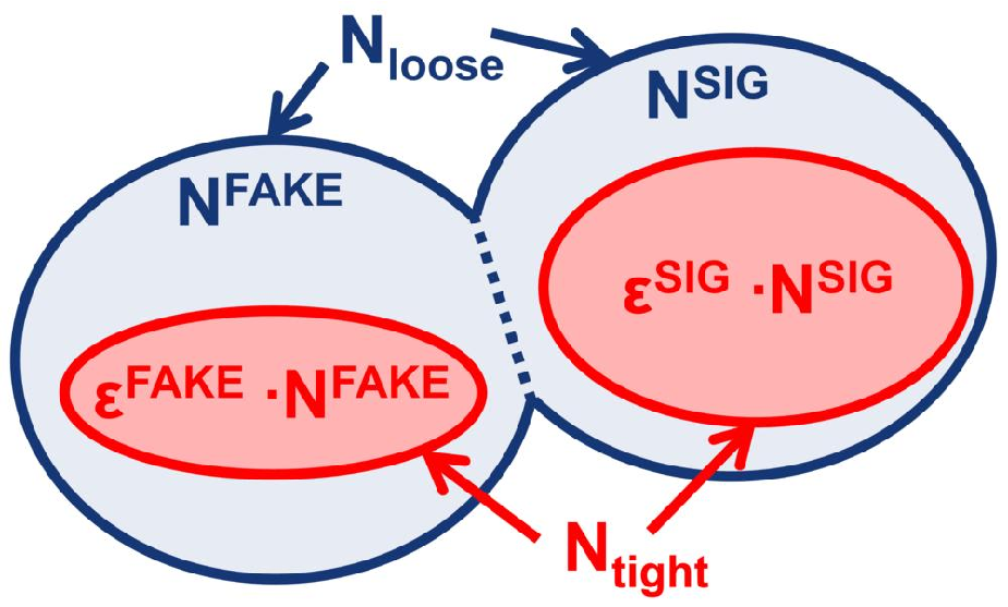
The linear system of two equations with two unknown variables can be rewritten as a matrix equation:

\left(\begin{array}[]{c}N_{\rm{loose}}\\ N_{\rm{tight}}\end{array}\right)=\left(\begin{array}[]{cc}1&1\\ \varepsilon^{\rm{sig}}&\varepsilon^{\rm{fake}}\end{array}\right)\left(\begin{array}[]{c}N^{\rm{sig}}\\ N^{\rm{fake}}\end{array}\right)

(4)

Solving the matrix equations yields the signal and background contributions in the data sample prior to the isolation cut:

	$\displaystyle N^{\rm{fake}}$	$\displaystyle=$	$\displaystyle\frac{N_{\rm{tight}}-\varepsilon^{\rm{sig}}N_{\rm{loose}}}{\varepsilon^{\rm{fake}}-\varepsilon^{\rm{sig}}},$		(5)
	$\displaystyle N^{\rm{sig}}$	$\displaystyle=$	$\displaystyle\frac{\varepsilon^{\rm{fake}}N_{\rm{loose}}-N_{\rm{tight}}}{\varepsilon^{\rm{fake}}-\varepsilon^{\rm{sig}}}.$		(6)

In order to determine the background contribution in the signal region (which corresponds to the tight selection by construction), the fraction of $N^{\rm{fake}}$ in the tight sample can be calculated using Equation 5 as

	$\displaystyle N_{\rm{tight}}^{\rm{fake}}$	$\displaystyle=$	$\displaystyle\varepsilon^{\rm{fake}}N^{\rm{fake}}$		(7)
		$\displaystyle=$	$\displaystyle\frac{\varepsilon^{\rm{fake}}}{\varepsilon^{\rm{sig}}-\varepsilon^{\rm{fake}}}\left(\varepsilon^{\rm{sig}}N_{\rm{loose}}-N_{\rm{tight}}\right).$		(7)

If the selection probabilities $\varepsilon^{\rm{sig}}$ and $\varepsilon^{\rm{fake}}$ for signal and background, respectively, are sufficiently different, the overall contribution of the QCD multijet background can be used to determine event based weights for the used data sample in order to obtain the distributions of the QCD multijet background contribution in arbitrary variables. This is done by assigning a weight to each data event based on the chosen requirement and the corresponding signal and fake probabilities of the objects taken into account for a given event. If it passes the loose selection only, the event weight is given by setting $N_{\rm{loose}}=1$ , $N_{\rm{tight}}=0$ in Equation 7, yielding

w_{\text{loose}}=\frac{\varepsilon^{\rm{sig}}\varepsilon^{\rm{fake}}}{\varepsilon^{\rm{sig}}-\varepsilon^{\rm{fake}}}.

(8)

Similarly, if both the loose and tight requirements are fulfilled, the event weight is given by setting $N_{\rm{loose}}=1$ , $N_{\rm{tight}}=1$ in Equation 7:

w_{\text{tight}}=\frac{\left(\varepsilon^{\rm{sig}}-1\right)\varepsilon^{\rm{fake}}}{\varepsilon^{\rm{sig}}-\varepsilon^{\rm{fake}}}.

(9)

This approach allows for a purely data driven estimation of both the normalisation and the shape of the QCD multijet background in semileptonic decays of top quark pairs. The individual parameters that have been used in the estimation for both the muon and electron channels in this analysis will be covered in the following sections. In addition, detailed studies of the performance and stability of the methods used will be demonstrated for the muon+jets channel alongside with an approach to obtain well-defined statistical and systematic uncertainties on the estimate.

1 Muon+jets Channel

In order to estimate the contribution from QCD multijet fake muons, the matrix method was applied to data in the QCD multijet-enriched low- $m_{\rm{T}}(W)$ control region. Furthermore, an inverted triangular cut was imposed to achieve orthogonality to the signal region in the determination of the fake probabilities $\varepsilon^{\rm{fake}}$ used in the Matrix Method:

m_{\rm{T}}(W)<20\,\rm{GeV}\text{ and }\not\!\!E_{\rm{T}}+m_{\rm{T}}(W)<60\,\rm{GeV}.

The impact of the described requirements on the QCD multijet estimate and the simulated $t\bar{t}$ signal is shown in Figure 2.

The signal probabilities $\varepsilon^{\rm{sig}}$ were determined in the signal region using a ${{Z/\gamma^{*}\rightarrow\mu\mu}}$ Tag & Probe method in order to select prompt muons from $Z$ decays.

The loose selection was identical to the full selection applied in the signal region (for details on the individual requirements, refer to Chapter 3 and Chapter 4), except for the muon isolation. The tight selection in addition requires isolation criteria based on both momentum and energy depositions around the muon tracks,

p_{\rm{T,cone30}}<4.0\,\rm{GeV}\text{ and }E_{\rm{T,cone30}}<4.0\,\rm{GeV},

corresponding to the full analysis event selection.

The fake probabilities have been obtained separately both with and without explicitly requiring at least one $b$ tagged jet ( $\geq 0$ $b$ tags and $\geq 1$ $b$ tags, respectively). In addition, the fake probabilities have been determined requiring at least two $b$ tagged jets, for completeness. For the latter cases, the JetFitCombNN $b$ tagging algorithm with a working point of $w=0.35$ (corresponding to an overall $b$ tagging efficiency of 70 %) has been used in accordance with the signal region event selection. Furthermore, the signal muon contribution from $W$ +jets and $Z$ +jets in the control region was obtained from Monte Carlo and subtracted to obtain a purer QCD multijet estimation. This contamination was of the order of 1.7 % ( $\geq 0$ $b$ tags) and 1.8 % ( $\geq 1$ $b$ tags).

In order to verify the stability of the method, the signal and fake (both without and with the requirement of at least one $b$ tagged jet) probabilities are shown as a function of the relative run number (full dataset with GoodRunsList applied) in Figure 3.

As can be seen, neither signal nor fake probabilities showed any significant trend with respect to run number and therefore, to instantaneous luminosity and different pile-up conditions.

In order to take into account dependencies on object kinematics, the signal and fake probabilities have been determined as a function of muon pseudorapidity $\eta$ to reflect the dependency on the muon detector acceptance. Furthermore, they have been parametrised as a function of the leading jet transverse momentum $p_{\rm{T}}(j_{1})$ in order to take into account the effects of hard jets and hence increased hadronic activity on the muon isolation. The respective projections for muon $\eta$ and $p_{\rm{T}}(j_{1})$ can be found in Figure 4.

The event yields and fractions in the signal region, obtained on a dataset corresponding to $1.04\,\rm{fb}^{-1}$ for different amounts of reconstructed jets required in the event selection (jet bins) can be found in Table 1.

Jet bin	$\geq 0$ $b$ tags		$\geq 1$ $b$ tags		$\geq 2$ $b$ tags
Jet bin	Yield	Fraction	Yield	Fraction	Yield	Fraction
1 jet	36820.5	5.6 %	3534.3	15.2 %	0.0
2 jet	14915.9	8.9 %	2633.3	17.0 %	106.6	9.5 %
3 jet	4141.8	9.6 %	1003.8	11.1 %	80.5	4.0 %
4 jet	1109.3	8.2 %	348.7	6.4 %	34.8	1.6 %
4 jet (incl.)	$1514.9_{-31.9\%}^{+31.8\%}$	7.7 %	$519.3_{-36.2\%}^{+36.2\%}$	5.6 %	$72.7_{-83.3\%}^{+83.3\%}$	1.8 %

Table 1: Event yields and fractions in the signal region for a dataset corresponding to

1.04\,\rm{fb}^{-1}

. Uncertainties correspond to the overall normalisation uncertainty due to statistical uncertainties from the obtained signal and fake probabilities, a second control region, the systematic shift of the

m_{\rm{T}}(W)

cut and the MC uncertainty on the

W

Z

+jets normalisation used in the subtraction of real leptons in the control region. The tagged probabilities correspond to the JetFitCombNN

b

tagging algorithm with a working point of

w=0.35

The following sources of systematic uncertainty have been taken into account in the estimate and were combined to a single uncertainty on the event weight, which can hence be propagated into a bin-by-bin normalisation and shape uncertainty on an arbitrary variable:

•

Statistical uncertainty on the signal and fake probabilities: Takes into account the uncertainties on both the signal and fake probabilities. The resulting uncertainty on the obtained event weights was evaluated using Gaussian error propagation. Note that the assumption of a symmetric probability distribution function was valid for the signal probabilities as well despite the closeness to unity, owing to the high statistics available from ${{Z/\gamma^{*}\rightarrow\mu\mu}}$ and the resulting small impact on the overall statistical uncertainty.
•

Systematic uncertainty from second control region: A second control region (high $d_{0}$ significance) was used for the fake probabilities to determine a bin-by-bin systematic discrepancy which was quoted as additional uncertainty on the event weight.
•

Systematic uncertainty due to choice of control region cut: The low transverse $W$ mass control region cut was varied by $5\,$ GeV up and down to estimate the impact on the obtained probabilities and event weights.
•

Uncertainties on $\bm{W}$ / $\bm{Z}$ +jets Monte Carlo normalisation: For the 1 jet inclusive bin, the $W$ / $Z$ +jets Monte Carlo normalisation uncertainties (25 %) were used to quantify the effect on the subtraction of real leptons in the control region.

The resulting overall normalisation uncertainties are shown in Table 1 for the signal region ( $\geq 4$ jets selection).

2 Electron+jets Channel

The QCD multijet contribution in the electron+jets channel has been estimated in analogy to the muon+jets channel, following slightly different criteria corresponding to the loose and tight selections[183]. The signal probabilities used in the Matrix Method were determined in the signal region with a ${{Z/\gamma^{*}\rightarrow ee}}$ Tag & Probe method in order to select prompt electrons from the $Z$ decay.

The fake probabilities have been determined in the QCD multijet-enriched low- $\not\hskip-2.84544ptE_{\rm{T}}$ control region:

5\,\rm{GeV}~<~\not\!\!E_{\rm{T}}~<~20\,\rm{GeV}.

Similar to the evaluation in the muon+jets channel, the loose selection was identical to the full selection applied in the signal region, except for the electron isolation criteria, which was modified in the loose selection:

\displaystyle E_{\rm{T,cone20}}

\displaystyle<

\displaystyle 6.0\,\rm{GeV},

while the tight selection requires

\displaystyle E_{\rm{T,cone20}}

\displaystyle<

\displaystyle 3.5\,\rm{GeV}.

In addition, slightly less stringent track quality criteria and the corresponding $\not\hskip-2.84544ptE_{\rm{T}}$ definition were applied to the reconstructed electron candidates in the loose sample with respect to the tight sample.

Furthermore, a subtraction of the real lepton contribution in the control region has been performed using the corresponding Monte Carlo predictions, in analogy to the muon+jets channel treatment.

4 Data Driven Estimation of the $W$ +jets Contribution

Due to the fact that the parton density of $u$ quarks in the protons brought to collision in the LHC is on average higher than the parton density of $d$ quarks (which can be observed already at lower momentum transfers, as depicted in Figure 5), a higher rate of $W^{+}$ than of $W^{-}$ is expected at the LHC. Since the production rates and the asymmetry in the production of $W^{+}$ and $W^{-}$ events has been determined to a higher theoretical precision[189, 190] than the overall $W$ +jets rate at the LHC, the observed $W^{+}/W^{-}$ asymmetry in data can be used to obtain an estimate for the rate of the $W$ +jets background contribution in the signal region[183].

Assuming that all processes other than the $W$ +jets production are symmetric in the final state lepton charge, the total number of $W$ +jets events, $N_{W}$ , can be extracted from the amount of observed data events passing the selection criteria described in Chapter 4 (except for the requirement of at least one $b$ tagged jet) with a positively (negatively) charged lepton, given by $D^{+}$ and $D^{-}$ , respectively:

	$\displaystyle N_{W}$	$\displaystyle=$	$\displaystyle N_{W^{+}}+N_{W^{-}}$		(10)
		$\displaystyle=$	$\displaystyle\left(\frac{r_{\text{MC}}+1}{r_{\text{MC}}-1}\right)\left(D^{+}-D^{-}\right).$		(10)

The fraction

r_{\text{MC}}=\frac{\sigma_{pp\rightarrow W^{+}}}{\sigma_{pp\rightarrow W^{-}}}

(11)

has been evaluated on Monte Carlo, based on the same event selection, and has been determined to be $1.56\pm 0.06$ in the electron+jets channel and $1.65\pm 0.08$ in the muon+jets channel, respectively. The dominant contributions to the overall uncertainty were due to PDF and jet energy scale uncertainties, and by the uncertainties on the heavy quark contribution fractions (i.e. the relative contributions from $Wb\bar{b}$ +jets, $Wc\bar{c}$ +jets and $Wc$ +jets).

Furthermore, the obtained overall $W$ +jets rate $N_{W}$ has been extrapolated to the full event selection by determining the relative fraction of events passing the requirement of at least one $b$ tagged jet after requiring exactly two reconstructed jets, $f_{2,\geq 1b\text{ tag}}$ , on data, and by determining the ratio $k_{2\rightarrow\geq 4}$ of the same fraction for the sample where at least four reconstructed jets were required with respect to $f_{2,\geq 1b\text{ tag}}$ , using the $W$ +jets Monte Carlo prediction[184]:

N_{W,\geq 1b\text{ tag}}=N_{W}\cdot f_{2,\geq 1b\text{ tag}}\cdot k_{2\rightarrow\geq 4}.

(12)

The fraction $f_{2,\geq 1b\text{ tag}}$ has been measured to be $0.063\pm 0.005$ in the electron+jets channel and $0.068\pm 0.005$ in the muon+jets channel, including statistical and systematic uncertainties. The extrapolation factor $k_{2\rightarrow\geq 4}$ has been determined to be $2.52\pm 0.36$ in the electron+jets channel and $2.35\pm 0.34$ in the muon+jets channel, respectively. The uncertainties include contributions from the statistical limitation of the used Monte Carlo samples and systematic uncertainties.

Chapter 6 Kinematic Event Reconstruction

As described in Chapter 4, the signature of a $t\bar{t}$ event in the semileptonic decay channel at leading order is the observation of four reconstructed jets, one isolated lepton and missing transverse energy. A reconstruction of the full $t\bar{t}$ final state was performed following a likelihood approach. A probability for the observation of a set of measured quantities under the assumption of a specific model and a set of model parameters was assigned. In this particular case, the model described the $t\bar{t}$ decay and the input quantities were the measured energies of the four jets, the measured energy of the lepton, and the missing transverse energy. The fit parameters of the likelihood were the parton energies, the lepton transverse momentum and the three neutrino momentum components. The likelihood was used to assign the measured jets to the decay products of the $t\bar{t}$ system. For this study, all permutations with four out of the five leading jets (if exist) were taken into account for the event reconstruction to increase the probability of identifying the proper combination in the presence of additional jets (e.g. from ISR or pile-up). Moreover, the (non-Gaussian) partonic energy resolution (the resolution of the particle jets with respect to the partons) of the final state objects were taken into account through the use of object specific transfer functions in order to obtain the final likelihood:

$\displaystyle L$	$\displaystyle=$	$\displaystyle\mathcal{B}(\widetilde{E}_{\rm{p,}1},\widetilde{E}_{\rm{p,}2}\|m_{W},\Gamma_{W})\cdot\mathcal{B}(\widetilde{E}_{\rm l},\widetilde{E}_{\nu}\|m_{W},\Gamma_{W})\cdot$	(1)
		$\displaystyle\mathcal{B}(\widetilde{E}_{\rm{p,}1},\widetilde{E}_{\rm{p,}2},\widetilde{E}_{\rm{p,}3}\|m_{t},\Gamma_{t})\cdot\mathcal{B}(\widetilde{E}_{\rm l},\widetilde{E}_{\nu},\widetilde{E}_{\rm{p,}4}\|m_{t},\Gamma_{t})\cdot$
		$\displaystyle\mathcal{W}(\hat{E}_{x}^{miss}\|\widetilde{p}_{x,\nu})\cdot\mathcal{W}(\hat{E}_{y}^{miss}\|\widetilde{p}_{y,\nu})\cdot\mathcal{W}(\hat{E}_{\rm{lep}}\|\widetilde{E}_{\rm{lep}})\cdot$
		$\displaystyle\prod_{\rm{i=1}}^{4}\mathcal{W}(\hat{E}_{\rm{jet,}i}\|\widetilde{E}_{\rm{p,}i})\cdot P(\textrm{$b$ tag}~\|~\textrm{quark}),$

where:

•

the $\mathcal{B}$ s represent the Breit-Wigner parametrisation of the parton (from which the associated jets originated) energies $\widetilde{E}_{\rm{p,}i}$ and lepton energies $\widetilde{E}_{\rm{lep}}$ with respect to the fitted ones,
•

the $\mathcal{W}$ s are the transfer functions associating the measured jets/leptons to the partonic objects, where the mapping functions of the objects are parametrised with a double Gaussian,
•

the $m_{W}$ and $\Gamma_{W}$ denote the $W$ boson mass and its decay width. The parameters are fixed to $m_{W}=80.4\,\rm{GeV}$ and $\Gamma_{W}=2.1\,\rm{GeV}$ , respectively,
•

the $m_{t}$ and $\Gamma_{t}$ denote the top quark pole mass and its decay width. The parameters were fixed to $m_{t}=172.5\,\rm{GeV}$ and $\Gamma_{t}=1.5\,\rm{GeV}$ , respectively,
•

the $\widetilde{X}$ are the partonic object quantities and $\hat{X}$ their corresponding measured values,
•

$P(\textrm{$b$ tag}~|~\textrm{quark})$ is a $b$ tag probability or rejection efficiency, depending on the quark flavor.

The probability $P(\textrm{$b$ tag}~|~\textrm{quark})$ was used to take into account the tagging efficiency and rejection rate of the used $b$ tagging algorithms at a specific working point.

The most probable event topology hypothesis was chosen by iterating over all possible permutations of reconstructed jets, the lepton and the missing energy and by maximising the logarithmic likelihood, $\log{L}$ . The permutation with the highest event probability was used for all further studies. The reconstruction efficiency, obtained in simulations, is shown for both the muon+jets and electron+jets channel in Figure 1.

As can be seen, the overall efficiencies for the reconstruction of the correct event topology (All Correct) in both channels were 62 % (74 %) with a fixed mass parameter, without (with) $b$ tagging information taken into account. In order to associate the reconstructed objects with the corresponding truth quarks and leptons, a simple $\Delta R$ matching was applied, using cone sizes of $0.3$ for jets and $0.1$ for leptons. An event was considered matched if all truth partons originating from the hard scattering process could successfully be identified with reconstructed jets and the truth lepton was matched to a reconstructed one. For the shown performance evaluation, only events where the four reconstructed jets and the lepton were successfully matched to corresponding truth level objects (contributing positively to the reconstruction efficiency) were taken into account. The matching efficiency on simulated $t\bar{t}$ events was about 30 % in both channels.

Examples for the transfer functions used in the likelihood can be found in Figure 2 and Figure 3, where the fit functions in different energy regions for $b$ jets in the pseudorapidity range $|\eta|<0.8$ and for electrons in the pseudorapidity range $0.8<|\eta|<1.37$ are shown.

A double Gaussian function was used in the fit of the transfer functions:

\displaystyle W(E_{\mathrm{true}},E_{\mathrm{reco}})=\frac{1}{2\pi(p_{2}+p_{3}p_{5})}(e^{-\frac{(\Delta E-p_{1})^{2}}{2p_{2}^{2}}}+p_{3}e^{-\frac{(\Delta E-p_{4})^{2}}{2p_{5}^{2}}}),

(2)

where the parameters $p_{1}$ , $p_{2}$ , $p_{3}$ , $p_{4}$ and $p_{5}$ are functions of the true energy of the respective particle and $\Delta E=E_{\mathrm{true}}-E_{\mathrm{reco}}$ .

Chapter 7 Unfolding

Any measured observable is influenced by imperfections of the used measurement apparatus and procedure itself, such as limited resolution of the detector response, the detector acceptance and possible object and event selections which are applied to the data. Due to these distortions, any measurement of such observable does not fully represent the original (or true) quantity. Mathematically, the actual measurement can be considered to be a convolution of the true quantity with a function representing the overall detector and selection acceptance and the detector response.

Let the true quantity be represented by a vector $\smash{\vec{t}}$ (with entries $t_{j}$ and $j=1,2,...,n_{t}$ ) describing the bin contents of a histogram, and the measured or reconstructed distribution by a corresponding vector $\smash{\vec{k}}$ (with entries $k_{i}$ and $i=1,2,...,n_{k}$ ), respectively. The underlying detector resolution effects can be described by a transition or response matrix $R^{\text{res}}$ , which contains the individual transition probabilities and hence the migrations between the observed elements of the distribution and the corresponding true values.

Furthermore, the detector acceptance and applied selection can be quantified by an additional weight factor for each element of $R^{\text{res}}$ , taking into account the probability of events from a particular entry of $\smash{\vec{t}}$ being observed at all in the measurement process. This additional correction, which can be described by a second matrix $R^{\text{acc}}$ , together with the response matrix describing the resolution effects, yields the overall response matrix $R$ :

R=R^{\text{acc}}R^{\text{res}},

(1)

denoting the transition probabilities between the observed distribution and the true distribution:

\vec{k}=R\vec{t},

(2)

where

	$\displaystyle R_{ij}$	$\displaystyle=$	$\displaystyle P(\text{observed in bin }i~\|~\text{expected in bin }j)$		(3)
		$\displaystyle=$	$\displaystyle P(k_{i}\|t_{j}).$		(4)

The concept of unfolding is illustrated in Figure 1, where an example distribution for an arbitrary variable $x$ is shown at the different stages in the measurement process.

In order to find an estimator for the true distribution given the measured distribution, an unfolding method[191] can be applied to correct for the respective acceptance and resolution effects. In this process, the response matrix is derived from an arbitrary reference sample, typically using Monte Carlo simulations. This procedure is called the training step of the unfolding. The obtained response matrix has to be inverted in order to allow the unfolding of any measured distribution to its corresponding true distribution. Since the response matrix represents the full resolution and acceptance information of the underlying measurement, the unfolding procedure can be performed model-independently, assuming that the detector simulation used in the training sample is sufficiently accurate.

However, in most situations where unfolding is applied, an exact and unique inverse response matrix $R^{-1}$ does not necessarily have to exist, such that

RR^{-1}=I,

(5)

where $I$ is the unity matrix. Hence, approximations are needed to perform the above matrix inversion to acceptable accuracy.

Limited statistics in the reference sample and the resulting statistical fluctuations can lead to additional and inadvertent bin migration effects in the response matrix, which do not represent the underlying resolution and acceptance effects. Consequently, these contributions have to be suppressed in the matrix inversion process, achieved by applying a regularisation procedure in order to limit the propagation of statistical fluctuations into the unfolded distribution or quantity. This regularisation typically involves a cut-off or weight parameter representing the sensitivity of the unfolding approach with respect to short-ranged bin-by-bin changes. Hence, the regularisation can be regarded as a constraint on the smoothness of the response matrix and hence the unfolded distribution.

The obtained approximate inverse matrix $R^{-1}$ is applied to the distribution measured from data, $\smash{\vec{m}}$ , and the respective unfolded distribution, $\smash{\vec{u}}$ , is obtained as estimator for the true distribution based on the given measurement:

\vec{u}=R^{-1}\vec{m}.

(6)

Several procedures have been developed to perform the inversion of the response matrix and the necessary regularisation. These unfolding methods will be briefly explained and evaluated with respect to their value and applicability for the measurement of the charge asymmetry using the observable $A_{C}$ in the following.

•

Bin-by-bin correction - Neglecting bin migrations, a simple reweighting can be performed by defining a correction factor for each bin of the distribution measured on data based on the true and measured reference distributions[192]:

$c_{i}=\frac{t_{i}}{k_{i}}.$ (7)

Consequently, the unfolding is performed by application of the respective correction factors to the corresponding bins of the distribution $\smash{\vec{m}}$ obtained from the data measurement to obtain the unfolded distribution $\smash{\vec{u}}$ :

$u_{i}=c_{i}\cdot m_{i}.$ (8)

Despite the simplicity of this method, it is prone to biases due to the reference Monte Carlo used in the training step, in particular the shape of the respective distributions. Since a priori no bin migrations are taken into account, it relies strongly on the correct description of the underlying physics and hence does not provide a model-independent approach. Furthermore, ambiguities in the determination of the statistical uncertainties may arise for cases where $k_{i}>t_{i}$ , where the obtained relative uncertainty can be underestimated, being smaller than the expected uncertainty for an ideal detector (i.e. where $m_{i}$ would itself be an estimator of $t_{i}$ ).
•

Singular value decomposition - This method employs a singular value decomposition (SVD) approach[193] in order to perform the inversion of the response matrix in the unfolding procedure. Singular value decomposition of a given real $m\times n$ matrix $R$ involves a factorisation such that

$R=USV^{T},$ (9)

where $U$ and $V$ denote $m\times m$ and $n\times n$ orthogonal matrices, respectively, such that $UU^{T}=U^{T}U=I_{m}$ and $VV^{T}=V^{T}V=I_{n}$ (with $I_{m}$ and $I_{n}$ being the corresponding $m\times m$ and $n\times n$ unity matrices). Furthermore, $S$ denotes an $m\times n$ diagonal matrix with non-negative diagonal elements, i.e. $S_{ij}=0$ for $i\neq j$ and $S_{ii}=s_{i}\geq 0$ . The matrix entries $s_{i}$ are called singular values of the matrix $R$ .

This form can be used in order to decompose the given measured distribution $\smash{\vec{k}}$ and the unknown true distribution $\smash{\vec{t}}$ into a series of orthogonal and normalised functions of the respective $m$ and $n$ classes by performing an appropriate rotation of the respective vectors. Consequently, the given initial system of linear equations as shown in Equation 2 is reduced to a diagonal system of equations, such that

$U^{T}\vec{k}=SV^{T}\vec{t}\quad\quad\Leftrightarrow\quad\quad\vec{d}=S\vec{z},$ (10)

where $\smash{\vec{d}}$ and $\smash{\vec{z}}$ denote the rotated measured and true vectors, respectively. This procedure is in particular effective if the respective singular values $s_{i}$ are small and the statistical uncertainties on the entries of the measured distribution are large, since in such a case any exact inversion solution is dominated by statistical fluctuations and thus physically meaningless.

By transformation of the given system of linear equations into the form of a weighted least squares minimisation, taking into account measurement uncertainties, a regularisation of the unfolding procedure can be achieved by the addition of a corresponding regularisation or stabilisation term to the expression to be minimised[194, 195, 196]. This introduces prior knowledge of the given problem and involves the requirement of minimal curvature of the obtained unfolded solution (i.e. the smoothness of the resulting distribution), eliminating statistical bin-to-bin fluctuations similar to the suppression of high-frequency harmonics in Fourier analysis. A regularisation parameter $\tau$ defines the relative weight of the additional regularisation term with respect to the terms originating from the given system of linear equation in the minimisation:

$\left(R\vec{t}-\vec{k}\right)^{T}\left(R\vec{t}-\vec{k}\right)+\tau\left(C\vec{t}\right)^{T}C\vec{t},$ (11)

where $C$ denotes a matrix representing the prior condition on the solution.

•

Bayesian iterative unfolding - A procedure based on an iterative approach to perform the inversion of the response matrix following Bayes’ theorem is applied[197]. This approach allows incorporating new knowledge to update a prior probability of observation of a given event[198, 199, 200] in an iterative procedure.

In order to obtain the inverted response matrix, the posterior probability of obtaining the true distribution $\vec{t}$ given the measured distribution $\vec{k}$ is calculated accordingly, assuming prior knowledge $P_{0}(t_{j})$ for the individual components of $\vec{t}$ based on the true distribution obtained in the Monte Carlo training step of the unfolding:

P(t_{j}|k_{i})=\frac{P(k_{i}|t_{j})P_{0}(t_{j})}{\sum_{l=1}^{n_{t}}P(k_{i}|t_{l})P_{0}(t_{l})}.

(12)

Note that in this context, the probability $P(k_{i}|t_{j})$ is identical to the transition probability $R_{ij}$ contained in the response matrix.

The obtained posterior probability distribution function is used as a prior in the next iteration, consecutively updating the existing knowledge about the respective probabilities with increasing number of iterations:

$\displaystyle P_{1}(t_{j})$	$\displaystyle\propto$	$\displaystyle\sum_{i}P(t_{j}\|k_{i})\cdot k_{i}\propto\sum_{i}P(k_{i}\|t_{j})\cdot P_{0}(t_{j})\cdot k_{i}$	(13)
$\displaystyle P_{2}(t_{j})$	$\displaystyle\propto$	$\displaystyle\sum_{i}P(t_{j}\|k_{i})\cdot k_{i}\propto\sum_{i}P(k_{i}\|t_{j})\cdot P_{1}(t_{j})\cdot k_{i}$	(14)
$\displaystyle P_{3}(t_{j})$	$\displaystyle\propto$	$\displaystyle\sum_{i}P(t_{j}\|k_{i})\cdot k_{i}\propto\sum_{i}P(k_{i}\|t_{j})\cdot P_{2}(t_{j})\cdot k_{i}$	(15)

Regularisation of the Bayes iterative unfolding procedure can be achieved naturally by restricting the number of iterations $N_{\text{It}}$ such that the underlying true distribution is recovered within the statistical uncertainties, and bin-to-bin fluctuations which are of purely statistical nature are suppressed. For a large number of iterations, a convergent state is reached, yielding the true, but strongly fluctuating inverse of the response matrix (thus minimising any remaining systematic bias of the unfolded distribution at the cost of larger statistical uncertainties). The number of iterations necessary to reach convergence depends on different conditions, including the choice of binning, the strength of bin migrations in the response matrix (i.e. the magnitude of its off-diagonal elements), and the choice of prior. The optimal choice of $N_{\text{It}}$ is case dependent and must be determined following a well-defined procedure, balancing remaining bias and statistical uncertainty of the obtained result.

Due to the fact that the bin-by-bin unfolding cannot account for bin migrations and does not allow for a regularised unfolding procedure, and hence is expected to be heavily model-dependent, this procedure was not eligible for the usage in this analysis. It only allows for a comparison of the measured asymmetry with the Standard Model prediction (unless the unfolding is performed for different model hypotheses), which can be achieved using the measured asymmetry directly as well.

The SVD unfolding approach, despite providing a well defined methodology, cannot perform an unfolding in more than one parameter in its current technical implementations, which would limit the analysis to an inclusive unfolding in a single parameter.

Given the requirements of the measurement, a Bayesian iterative unfolding was performed in this analysis in order to recover the inclusive $|y_{t}|-|y_{\bar{t}}|$ distribution and the resulting charge asymmetry observable $A_{C}$ at the parton level. In particular, this approach allowed for a simultaneous unfolding in multiple observables due to the fact that Bayesian unfolding is independent of the ordering of the classes/bins. Since many of the BSM models summarised in Chapter 1 predict different magnitudes of the charge asymmetry for low and high $M_{t\bar{t}}$ regions, a simultaneous unfolding of $|y_{t}|-|y_{\bar{t}}|$ and the invariant $t\bar{t}$ mass, $M_{t\bar{t}}$ , has been performed, taking into account bin migrations in both dimensions. Semileptonic $t\bar{t}$ events generated with the mc@nlo generator have been used as reference sample to obtain the response matrix based on the detector simulation. Furthermore, a simple extraction of the covariance matrix of the unfolded distributions[201] was possible.

The SVD unfolding was performed for the inclusive measurement as a cross-check to verify the stability and consistency of the Bayes iterative approach (c.f. Appendix 13).

The techniques utilised were available in the RooUnfold package[201], which provided simple interfaces and efficient implementations for all three mentioned unfolding methods.

Chapter 8 Systematic Uncertainties

In addition to the statistical uncertainty originating from limited data statistics, there were a multitude of systematic effects that can have an impact on the performed measurement. These effects were studied individually and a corresponding systematic uncertainty on the measurement result was assigned for each contribution.

In order to evaluate the individual effects, the analysis was performed for each systematic under consideration with a modified response matrix and/or background contribution depending on the modelled effect. The changes typically corresponded to an uncertainty of one or more parameters (e.g. a shift of the muon trigger efficiencies according to the respective uncertainties) or an alternate model (e.g. a different MC generator used for the simulation of $t\bar{t}$ events). The uncertainty was extracted in each case based on the shift in the measurement central value when changing the parameters accordingly, and was symmetrised.

In order to suppress the statistical component of the obtained uncertainty inherent in the re-evaluation of the central value by changing different parameters of the performed measurement, the requirement of at least one $b$ tagged jet in the event selection was replaced by a reweighting method. The $|y_{t}|-|y_{\bar{t}}|$ distribution for the Monte Carlo based background contributions ( $W$ +jets, $Z$ +jets, single top and diboson background) was obtained by direct application of the $b$ tag weights to the events passing the nominal event selection without the requirement of at least one $b$ tagged jet. This approach is very similar to the trigger reweighting approach described in Chapter 3. The same procedure was applied for the simultaneous unfolding in $|y_{t}|-|y_{\bar{t}}|$ and $M_{t\bar{t}}$ . Furthermore, the normalisation of the resulting distributions was modified to match the distribution obtained using the nominal event selection to avoid the introduction of a potential bias in the background subtraction. Control plots showing the agreement of the two approaches can be found in Appendix 15. Since the weighted distributions were compatible within statistical uncertainties with the nominal distributions, no additional systematic uncertainty was assigned. The bin-by-bin statistical uncertainty in the background distribution is reduced by up to 25 %.

The following systematics were considered and evaluated for this analysis. All contributions were assigned to the Monte Carlo prediction (signal and/or background, were applicable).

•

QCD multijet uncertainty - The QCD multijet background was estimated with data driven methods in both the electron and muon channel. Since both the shape and the overall normalisation of the estimation can only be verified to a limited extend, a very conservative systematic uncertainty of 100 % was quoted despite the availability of more advanced estimates (c.f. Chapter 1), following the recommendations of the performance groups. Results following a less conservative approach are discussed in Appendix 14. The QCD multijet background normalisation was shifted up and down by 100% to quantify this uncertainty. Since the QCD multijet background contribution is intrinsically charge symmetric, but enters the background subtraction, the normalisation and not shape was the dominant source of systematic uncertainty.
•

Jet energy scale - The jet energy scale (JES) uncertainty was derived using information from test beam data, LHC collision data and simulation and was taken into account by scaling up and down the energy of all considered jets by $1\,\sigma$ of the associated transverse momentum uncertainty based on the jet $p_{\rm{T}}$ and $\eta$ [202]. The full event selection and kinematic reconstruction has been re-run with the scaled jets. In addition, the missing transverse energy has been re-evaluated, taking into account the scaled contributions of the jets in $p_{x}$ and $p_{y}$ . For jets within the acceptance range, the JES uncertainty varied from about 2.5 % for high $p_{\rm{T}}$ jets in the central detector region to about 14 % for low $p_{\rm{T}}$ jets in the forward region.
•

Pile-up (JES) - Depending on the instantaneous luminosity and the amount of vertices, an event weight was assigned to match the pile-up contribution in the simulation to data. An additional systematic uncertainty of 5% (7%) for low $p_{\rm{T}}$ jets or 2% (3%) for high $p_{\rm{T}}$ jets in the $|\eta|<2.1$ ( $2.1<|\eta|<4.5$ ) region was added to the JES uncertainty in quadrature[203].
•

$\bm{b}$ jet energy scale - In order to account for the difference of the energy scale for $b$ jets with respect to light quark jets, all $b$ jets (i.e. jets which have a matched truth $b$ quark in simulations) were scaled by an additional fraction ranging from 2.5 % in the low $p_{\rm{T}}$ jet region to 0.76 % in the high $p_{\rm{T}}$ jet region and added to the JES uncertainty in quadrature[202].
•

Jet reconstruction efficiency - The jet reconstruction efficiency (JRE) was evaluated by randomly dropping jets from events with a probability of about 2%[167]. The resulting difference with respect to the nominal case was symmetrised and quoted as JRE systematic uncertainty.
•

Jet energy resolution - A smearing of the jet transverse momentum corresponding to a resolution of about 10 % was applied to Monte Carlo events as systematic to reflect the difference between the jet energy resolution (JER) observed on data and Monte Carlo[167]. The resulting discrepancies were symmetrised and quoted as JER systematic uncertainty.
•

Muon efficiencies - In order to account for the trigger and reconstruction efficiencies for muons[204, 205], global and object based scale factors and efficiencies were taken into account and a systematic uncertainty was assigned on an event-by-event basis (for global scale factors) or on an object basis. These were combined into an overall muon efficiency uncertainty of the order of 1 %. In addition, a one-sided uncertainty of 1.5 % (events with 0 or 1 $b$ tagged jet) or 2.2 % (events with more than 1 $b$ tagged jet) was assigned to the muon trigger efficiency to account for a mis-modelled and as a consequence discarded trigger object matching algorithm in the Monte Carlo samples.
•

Muon scales and resolution - Since the Monte Carlo muon momentum scales and resolution differed from the ones observed in data, the muon momentum was smeared and a scaling of up to 1.5 % was applied on object level to account for this discrepancy[171]. A systematic uncertainty at the sub-percent level was assigned by scaling up and down both the momentum scaling and smearing by 1 $\sigma$ according to the respective uncertainty. In addition, the missing energy was re-evaluated with the modified four-vector information. The full event selection and kinematic reconstruction was performed for the different scales, resulting in a symmetrised systematic uncertainty based on the comparison of the different results of the measurement.
•

Electron efficiencies - In order to account for the trigger and reconstruction efficiencies for electrons, global and object based scale factors were taken into account[172]. A systematic uncertainty was assigned on an event basis (for global scale factors) or on an object basis, which were combined into an overall electron efficiency uncertainty of the order of 1 %.
•

Electron scales and resolution - In order to take into account discrepancies between the electron energy resolution on Monte Carlo and data, a Gaussian smearing procedure was applied to the electron energy for Monte Carlo events to reflect the resolution in data[172]. In addition, the electron energy in data was corrected to account for a scaling mis-match between data and Monte Carlo. Both systematic uncertainties were of the order of 1 % to 2 % and were assigned to the Monte Carlo prediction for consistency.
•

$\bm{b}$ tag scale factors - Due to discrepancies in the $b$ tagging efficiencies and fake rates between data and simulation, all Monte Carlo jets were assigned a specific weight to account for this effect[206, 168]. The obtained $b$ tag weights for each jet were combined into an event weight by multiplication (corresponding to a logical AND of all jets taken into account). The provided scale factors contained uncertainties which result in small shape variations. In order to determine the deviation in the shapes from the nominal case due to the $b$ tag scaling and to quantify the corresponding systematic uncertainty on the measurement, the resulting samples were shifted up and down by the provided uncertainties. These were of the order of 8 %, depending on the jet $p_{\rm{T}}$ and $\eta$ .
•

PDF uncertainty - For the mc@nlo signal Monte Carlo, CTEQ6.6 PDFs were utilised to model the incoming partons to the hard scattering process, as described in Chapter 2. The impact of the choice of PDFs was evaluated by varying the eigenvalues of the CTEQ parametrisation[207] or by comparison with the respective MRST2001 parametrisation[208], using the Lhapdf tool[209]. Event weights were determined and the variations in the resulting pseudosamples were taken into account as PDF systematic uncertainty.
•

LAr defects - Parts of the LAr calorimeter readout electronics were inoperative during a significant time period of data taking due to a technical problem. Having occurred after the production of the used Monte Carlo samples, it was necessary to correct for the resulting mismatch between data and simulated events at the analysis level. Monte Carlo events were dropped with a probability corresponding to the relative amount of data affected (84.0 %) if an electron or a jet entered the region of degraded acceptance (taking into account the isolation requirements). A systematic uncertainty was assigned based on different transverse momentum requirements for the jets taken into account for this procedure after symmetrisation.
•

ISR and FSR - In order to take into account initial and final state radiation, which can introduce additional jets in the observed events, different Monte Carlo samples with varying ISR and FSR contributions[187] (ISR and FSR contributions scaled up and down independently and in combination) were evaluated by replacing the nominal signal sample in the measurement. The systematic uncertainty was quoted as the maximum relative deviation from the nominal leading order sample observed in these variations and applied to the mc@nlo prediction. The parameters were varied in a range comparable to those used in the Perugia Soft/Hard tune variations[210].
•

$\bm{t}\bar{\bm{t}}$ modelling - The impact of using different MC generators for the signal process modelling was studied. In addition to the mc@nlo generator, the powheg generator was used for comparison and a symmetrised systematic uncertainty was assigned based on the variations in the measurement results for the alternate modelling.
•

Parton shower / fragmentation - In addition to the matrix element level MC generator, the effect of different showering models was taken into account by comparing the results for the powheg generator with showering performed by pythia and by herwig, and a symmetrised systematic uncertainty was assigned based on the variations in the measurement results for the alternate shower modelling.
•

Top mass - Since the top mass parameter was considered fixed, the uncertainty on the measurement of the mass was taken into account separately. Two different Monte Carlo samples generated with different mass parameters (scaled up and down to 180 GeV and 170 GeV, respectively) were used and the observed deviations were linearly interpolated according to the actual uncertainty of 0.5 % of the top mass measurement[13] and a symmetrised systematic uncertainty was quoted.
•

$\bm{W}$ +jets background uncertainty - The W+jets background normalisation was estimated with a data driven method and a systematic uncertainty based on the limited statistics available and several systematic contributions to the method have been evaluated (see Chapter 4 for details). An overall $W$ +jets normalisation uncertainty of 22.4 % and 22.7 % was obtained in the muon+jets and electron+jets channel, respectively. In addition, the $W$ +jets background shape uncertainty has been evaluated by modifying several generator parameters such as the renormalisation scale or the functional form of the factorisation scale compared to the nominal alpgen parameters, based on the leading jet $p_{\rm{T}}$ . A symmetrised systematic uncertainty on the charge asymmetry measurement has been assigned based on the deviations for two different sets of parameters with respect to the nominal results.
•

$\bm{Z}$ +jets background uncertainty - In order to quantify the uncertainty on the $Z$ +jets contribution normalisation, a Berends-Giele scaling uncertainty[211] was calculated, corresponding to an overall normalisation uncertainty of 34 %. In addition, the $Z$ +jets background was determined independently from both the alpgen and sherpa generator to quantify the shape uncertainty, which was quoted based on the symmetrised discrepancy of the results obtained with sherpa with respect to the nominal case, in which alpgen samples were used.
•

Charge mis-identification - Since the detector momentum resolution is finite, and the lepton charge was identified by taking into account the bending radius of the particle track, a certain probability for mis-identifying the lepton charge exists, especially for high transverse momentum leptons due to their almost straight trajectories. This probability was evaluated on Monte Carlo and on data to be of the order of 0.2 % to 0.5 % in the central detector region, and up to 2.5 % in the forward region, respectively, in the electron+jets channel[183]. In the muon+jets channel, the probability was found to be below 0.003 % in all cases. A corresponding symmetrised systematic uncertainty on the measurement of the charge asymmetry was determined.
•

$\bm{b}$ tag charge - A dependency of the $b$ tag efficiencies on the $b$ quark charge can lead to a bias in the measurement due to the requirement of at least one $b$ tagged jet. Hence, a simple Monte Carlo study on parton level was performed by simulating a difference in the $b$ tag efficiency of 5 % between $b$ and $\bar{b}$ quarks. The resulting impact on the charge asymmetry on parton level was studied and the difference with respect to the nominal case (assuming identical tagging efficiencies for $b$ and $\bar{b}$ quarks) was quoted as systematic uncertainty.
•

MC generator statistics - Since the signal Monte Carlo sample entered directly into the unfolding response matrix and statistical fluctuations in the bins of this matrix can have an impact on the unfolding process, an additional ensemble test was performed by fluctuating the obtained nominal response matrix on a bin-by-bin basis following a Gaussian probability distribution (since the statistics from the mc@nlo sample were very high a Gaussian model could safely be assumed). Uncertainties of the order of 0.3 % to 3 % have been obtained, depending on the statistics in each bin of the response matrix.
•

Unfolding convergence - Based on the convergence evaluation which was used to determine the optimal amount of regularisation in the unfolding process (for details refer to Chapter 3), a remaining absolute uncertainty of 1 ‰, corresponding directly to the choice of convergence criterion, was assigned, representing the potential remaining change with respect to further increase in regularisation.
•

Unfolding bias - Closure tests have been performed using ensembles of pseudodata to quantify any remaining bias from the unfolding at the chosen regularisation strengths by obtaining pull distributions for the measured asymmetry, normalised with respect to the respective unfolding statistical uncertainty. The corresponding distributions can be found in Figure 8 in Appendix 11. The remaining bias was extracted from the residuals in the pull distributions in the closure tests and was taken into account as an additional systematic uncertainty. The residual bias after unfolding was extracted from the respective pull distributions corresponding to the regularisation used in the individual cases and taken into account as an additional relative uncertainty on the unfolded results, which was of the order of 1 % to 11 %.
•

Other backgrounds - For the small backgrounds from single top and diboson production, only normalisation uncertainties were considered. For the single top contribution, the uncertainties of the approximate next-to-next-to-leading order prediction (for details, refer to Chapter 2) were taken into account (corresponding to an uncertainty of about 11 %), while for the diboson production, an overall uncertainty of 5 % was assumed.
•

Luminosity - The relative uncertainty on the measurement of the integrated luminosity of the used data sample was estimated to be 3.7 %[212] and was taken into account for the measurement.
•

Pile-up - In order to take into account the difference in pile-up conditions between Monte Carlo and data, an event based reweighting was performed to reflect the distribution of average observed number of interactions per bunch crossing on data. The impact of the pile-up conditions on the measurement before unfolding is shown in detail in Chapter 3. Since no significant pile-up dependency was observed, no additional systematic uncertainty was assigned.

Chapter 9 Results

1 Event Yields & Control Plots

The final expected and observed number of events in both the muon+jets and the electron+jets channel after performing the event selection can be found in Table 1, both without and with the requirement of at least one $b$ tagged jet.

Channel	muon+jets						electron+jets
Selection	$\geq 0$ $b$ tags			$\geq 1$ $b$ tags			$\geq 0$ $b$ tags			$\geq 1$ $b$ tags
$t\bar{t}$	7187	$\!\!\!\pm\!\!\!$	588	6342	$\!\!\!\pm\!\!\!$	519	4832	$\!\!\!\pm\!\!\!$	395	4256	$\!\!\!\pm\!\!\!$	348
Single top	458	$\!\!\!\pm\!\!\!$	40	366	$\!\!\!\pm\!\!\!$	32	320	$\!\!\!\pm\!\!\!$	28	256	$\!\!\!\pm\!\!\!$	22
$W$ +jets (data)	8617	$\!\!\!\pm\!\!\!$	1173	1390	$\!\!\!\pm\!\!\!$	311	5407	$\!\!\!\pm\!\!\!$	768	883	$\!\!\!\pm\!\!\!$	200
$Z$ +jets	940	$\!\!\!\pm\!\!\!$	333	134	$\!\!\!\pm\!\!\!$	47	756	$\!\!\!\pm\!\!\!$	267	105	$\!\!\!\pm\!\!\!$	37
Diboson	134	$\!\!\!\pm\!\!\!$	7	22	$\!\!\!\pm\!\!\!$	2	80	$\!\!\!\pm\!\!\!$	5	13	$\!\!\!\pm\!\!\!$	1
QCD multijet (data)	1515	$\!\!\!\pm\!\!\!$	757	519	$\!\!\!\pm\!\!\!$	519	944	$\!\!\!\pm\!\!\!$	472	247	$\!\!\!\pm\!\!\!$	247
Total background	11663	$\!\!\!\pm\!\!\!$	1436	2431	$\!\!\!\pm\!\!\!$	608	7508	$\!\!\!\pm\!\!\!$	941	1504	$\!\!\!\pm\!\!\!$	321
Total expected	18850	$\!\!\!\pm\!\!\!$	1552	8774	$\!\!\!\pm\!\!\!$	799	12340	$\!\!\!\pm\!\!\!$	1020	5760	$\!\!\!\pm\!\!\!$	473
Observed	19639			9124			12096			5829

Table 1: Observed number of data events in comparison to the expected number of Monte Carlo signal events and different background contributions for the event selection, both with and without the requirement of at least one

b

tagged jet. The QCD multijet and

W

+jets contributions were estimated using data driven methods (c.f. Chapter 5). Uncertainties are statistical and include the respective systematic uncertainties on the normalisation for QCD multijet and

W

+jets and the cross-section uncertainties on all other contributions. For the QCD multijet background, a conservative 50 % (100 %) overall normalisation uncertainty for the selection without (with) requiring at least one

b

tagged jet was assumed.

Control plots for the full event selection as described in Chapter 4, showing a comparison of the observation and expectation for several object and event quantities, can be found in Figure 1 and Figure 2, for both the muon+jets and the electron+jets channel, respectively. The uncertainties on the expectation include statistical and the leading systematic uncertainties, that is QCD multijet background and $W$ +jets normalisation, luminosity, jet energy scale, $b$ tag scale factors and $t\bar{t}$ cross-section uncertainty.

Due to the tighter definition of selection criteria in the electron+jets channel, the number of events in the electron+jets channel was significantly lower than it was the case for the muon+jets channel. This was necessary in order to reduce the contribution from the increased number of electron fakes originating from the QCD multijet background with respect to the muon channel, where the expected fake rate was significantly lower. The overall agreement between Monte Carlo prediction and data was very good in both channels. Additional control plots for the same quantities without the explicit requirement of at least one $b$ tagged jet can be found in Figure 3 and Figure 4 of Appendix 11 for completeness.

In addition to the control plots showing basic object and event kinematics, several more complex quantities based on the kinematic event reconstruction, as described in Chapter 6, can be found in Figure 3. The respective distributions for the logarithmic likelihood of the kinematic fit, and the invariant mass and transverse momentum of the reconstructed $t\bar{t}$ system in both the muon+jets and the electron+jets channel are shown. The agreement between data and prediction is very good, indicating a proper modelling of the $t\bar{t}$ signal and background kinematics in the various Monte Carlo samples and data driven background estimates.

2 Measurement of the Charge Asymmetry

Events passing the described event selection were taken into account to determine the differential and integrated charge asymmetry based on the distribution of $|y_{t}|-|y_{\bar{t}}|$ . A subtraction of the predicted background contributions was performed on the distributions measured on data to obtain an estimate for the $t\bar{t}$ signal contribution only.

The corresponding distributions are shown in Figure 4 for both the inclusive measurement of the $|y_{t}|-|y_{\bar{t}}|$ distribution and the corresponding measurement for the two cases of $M_{t\bar{t}}<450$ GeV and $M_{t\bar{t}}>450$ GeV. For the $M_{t\bar{t}}$ dependent measurement, an additional requirement on the event reconstruction logarithmic likelihood of $\log{L}>-52$ (see Figure 3) has been applied in order to improve the resolution in the $t\bar{t}$ invariant mass. The respective relative resolution in $M_{t\bar{t}}$ for both channels before and after the application of the additional requirement on $\log{L}$ can be found in Figure 1 and Figure 2 in Appendix 11. The relative resolution improves from 28.8 % to 18.4 % in the muon+jets channel and from 28.8 % to 17.7 % in the electron+jets channel.

The resulting charge asymmetries for the observable $A_{C}^{\text{reco}}$ obtained after background subtraction can be found in Table 2 for both the muon+jets channel and the electron+jets channel. The observed results are shown alongside the predicted $t\bar{t}$ charge asymmetries obtained with mc@nlo for comparison. The uncertainties on the prediction correspond to the limited Monte Carlo statistics in the used sample after the applied selection.

Muon+jets Channel
Measurement	Observed	Predicted (mc@nlo)
Inclusive	$-0.010\pm 0.015\,\text{(stat.)}\pm 0.008\,\text{(syst.)}$	$\phantom{-}0.0021\pm 0.0011\,\text{(stat.)}$
$M_{t\bar{t}}<450$ GeV	$-0.012\pm 0.024\,\text{(stat.)}\pm 0.007\,\text{(syst.)}$	$-0.0043\pm 0.0018\,\text{(stat.)}$
$M_{t\bar{t}}>450$ GeV	$-0.011\pm 0.022\,\text{(stat.)}\pm 0.007\,\text{(syst.)}$	$\phantom{-}0.0064\pm 0.0015\,\text{(stat.)}$
Electron+jets Channel
Inclusive	$-0.034\pm 0.019\,\text{(stat.)}\pm 0.010\,\text{(syst.)}$	$-0.0003\pm 0.0014\,\text{(stat.)}$
$M_{t\bar{t}}<450$ GeV	$-0.060\pm 0.033\,\text{(stat.)}\pm 0.019\,\text{(syst.)}$	$\phantom{-}0.0007\pm 0.0022\,\text{(stat.)}$
$M_{t\bar{t}}>450$ GeV	$-0.032\pm 0.028\,\text{(stat.)}\pm 0.015\,\text{(syst.)}$	$-0.0010\pm 0.0017\,\text{(stat.)}$

Table 2: Measured values of the charge asymmetry observable

A_{C}^{\text{reco}}

for the muon+jets and electron+jets channel after subtraction of the various background contributions. The results for the inclusive measurement and the respective measurements for

M_{t\bar{t}}<450

GeV and

M_{t\bar{t}}>450

GeV are shown together with the mc@nlo predictions.

As can be seen in the table, the obtained results were compatible with the mc@nlo Standard Model prediction in all cases within the statistical and systematic uncertainties. However, in the electron+jets channel, a tendency towards more negative asymmetries was observed, in particular for the measurement of $A_{C}^{\text{reco}}$ for $M_{t\bar{t}}<450$ GeV. A breakdown of the individual systematic uncertainties taken into account can be found in Table 1 and Table 2 of Appendix 12 for completeness.

In addition, the integrated charge asymmetry $A_{C}^{\text{reco}}$ after background subtraction as a function of the invariant $t\bar{t}$ mass, $M_{t\bar{t}}$ is shown in Figure 5 together with the Standard Model prediction obtained from simulated $t\bar{t}$ events.

The observed asymmetry values show no statistically significant deviation from the Standard Model prediction. Since, in addition, no systematic uncertainties were included, the observed discrepancies are negligible.

3 Unfolding

In order to perform the Bayes iterative unfolding and to correct the measured differential and integrated charge asymmetry for detector resolution and acceptance effects, the corresponding response matrix has been obtained using the full set of $t\bar{t}$ signal Monte Carlo events generated with mc@nlo (15 000 000 simulated events). A unified binning for the true and reconstructed distributions (and consequently for the response matrices) in the variable $|y_{t}|-|y_{\bar{t}}|$ has been used, employing six bins with variable width to ensure sufficient statistics in the tails of the respective distributions. Bin edges at $\{-3.0,-1.2,-0.6,0.0,0.6,1.2,3.0\}$ for the inclusive unfolding and $\{-3.00,-0.96,-0.48,0.0,0.48,0.96,3.00\}$ for the simultaneous unfolding in $|y_{t}|-|y_{\bar{t}}|$ and $M_{t\bar{t}}$ were chosen.

Furthermore, for the simultaneous unfolding in $|y_{t}|-|y_{\bar{t}}|$ and $M_{t\bar{t}}$ , an additional requirement on the event reconstruction logarithmic likelihood of $\log{L}>-52$ (see Figure 3) has been applied in order to improve the resolution of the $t\bar{t}$ invariant mass in the same way as for the measurement of the charge asymmetry before unfolding.

The response matrix representation used in the inclusive measurement of the distribution of $|y_{t}|-|y_{\bar{t}}|$ and of $A_{C}^{\text{unf}}$ is shown in Figure 6 for both the muon+jets and electron+jets channel.

Similarly, the corresponding matrices for the simultaneous unfolding in $|y_{t}|-|y_{\bar{t}}|$ and $M_{t\bar{t}}$ can be found in Figure 7. The transition probability information of the corresponding two-dimensional distributions (with $2\times 6$ bins) was encoded in the matrix by linearisation of the respective histograms, concatenating the bins from the two $M_{t\bar{t}}$ regions into a single one dimensional histogram (with $1\times 12$ bins). Hence, the associated response matrix contained $2\times 2$ quadrants, corresponding to the transition probabilities for the true and reconstructed $|y_{t}|-|y_{\bar{t}}|$ distributions in the low and high $M_{t\bar{t}}$ regions of phase space, respectively.

A closure test has been performed to verify that the Bayesian iterative unfolding approach can be used to recover an arbitrary asymmetry present in the true distribution. The full mc@nlo $t\bar{t}$ signal sample was used as a basis to verify the correct unfolding response for different artificially injected truth level asymmetries. This was achieved by performing an event-by-event reweighting of the $t\bar{t}$ signal sample to asymmetries of -10 %, -5 %, 0 %, 5 % and 10 % in the variable $A_{C}^{\text{true}}$ by systematically increasing the weights of events with $|y_{t}|-|y_{\bar{t}}|<0$ and decreasing the weights of events with $|y_{t}|-|y_{\bar{t}}|>0$ by the same amount.

Pseudoexperiments, using statistically independent sets of pseudodata corresponding to the statistics expected in the used data sample (after background subtraction), were conducted based on a Poissonian fluctuation of the respective distribution in $|y_{t}|-|y_{\bar{t}}|$ , taking into account the additional event weights determined in the asymmetry reweighting. Ensemble tests were performed to confirm the linearity of the unfolding response in the true value of the chosen charge asymmetry observable $A_{C}^{\text{true}}$ . Furthermore, the dependency of the obtained results on the regularisation of the unfolding procedure was studied.

The average unfolded value of $A_{C}^{\text{unf}}$ obtained from the sets of pseudodata as a function of the injected true value of $A_{C}^{\text{true}}$ can be found for both the inclusive unfolding and the simultaneous unfolding in $|y_{t}|-|y_{\bar{t}}|$ and $M_{t\bar{t}}$ in Figure 8 for different regularisation strengths, using $N_{\text{It}}=5$ , 10, 20, 40 and 80 iterations in the Bayesian unfolding.

A straight line fit using a parametrisation of the form

A_{C}^{\text{unf}}=a\cdot A_{C}^{\text{true}}+b

(1)

has been performed, where $a$ and $b$ denote the slope and offset parameters, respectively. The procedure has been repeated for each of the individual choices of $N_{\text{It}}$ to obtain the calibration curves in order to verify the linearity and determine the respective slopes and offsets of the fit. These provided a measure for the average remaining bias in the unfolded differential and integrated asymmetry after unfolding for different regularisation strengths. As can be seen in the fits, a slope close to one could be achieved in all cases, indicating a proper average correspondence of the unfolded asymmetry to the injected true value, independent of the strength of the injected asymmetry.

In addition, the expected statistical uncertainty on $A_{C}^{\text{unf}}$ after the unfolding procedure is shown in Figure 5 in Appendix 11 as a function of $N_{\text{It}}$ . As expected, the uncertainty increases with the number of iterations used in the regularisation due to the increasing sensitivity to bin-to-bin statistical fluctuations in the inversion process of the response matrix. The expected uncertainties are independent of the injected value of $A_{C}^{\text{true}}$ .

In order to achieve a convergent state in the iterative unfolding process, the dependency of the unfolded result as a function of the number of iterations has been studied with respect to a defined convergence criterion. For individual ensembles of pseudodata, the unfolding procedure was considered to be converged if the absolute change in the unfolded asymmetry in terms of $A_{C}^{\text{unf}}$ , $\Delta A_{C}^{\text{unf}}$ , for a given amount of iterations $N_{\text{It}}=i$ with respect to the previous amount of iterations $N_{\text{It}}=i-1$ was lower than 1 ‰, i.e. if

\Delta A_{C}^{\text{unf}}=|A_{C}^{\text{unf}}(N_{\text{It}}=i)-A_{C}^{\text{unf}}(N_{\text{It}}=i-1)|<0.001.

(2)

Figure 6 in Appendix 11 shows the percentage of ensembles which have reached the defined convergence criterion as a function of regularisation strength, parametrised by the amount of iterations $N_{\text{It}}$ . At $N_{\text{It}}=40$ (inclusive unfolding), and $N_{\text{It}}=80$ (simultaneous unfolding in $|y_{t}|-|y_{\bar{t}}|$ and $M_{t\bar{t}}$ ) iterations, all ensembles of pseudodata were ensured to have reached convergence for all injected value of $A_{C}^{\text{true}}$ . Hence, these regularisation strengths were chosen for the inclusive unfolding and the simultaneous unfolding in $|y_{t}|-|y_{\bar{t}}|$ and $M_{t\bar{t}}$ , respectively. An additional systematic uncertainty of 1 ‰, corresponding directly to the choice of convergence criterion was assigned to the unfolded value of $A_{C}^{\text{unf}}$ (c.f. Chapter 8).

In addition, a further cross-check was performed to verify that the unfolding procedure reached a convergent state by determining the average standard deviation of the variable $\Delta A_{C}^{\text{unf}}$ for the used set of ensembles as a function of $N_{\text{It}}$ , which shows a monotonous falling behaviour in all cases as expected. The corresponding additional control plots can be found in Figure 7 in Appendix 11 for completeness.

Despite the large amount of iterations necessary to reach convergence, in particular for the simultaneous unfolding in $|y_{t}|-|y_{\bar{t}}|$ and $M_{t\bar{t}}$ and the associated expected statistical uncertainties, this approach allowed performance of the unfolding following a well-defined and model-independent procedure. Furthermore, the remaining expected bias in the unfolding procedure was minimised, as can be seen in the calibration curves in Figure 8 for the used choices of $N_{It}=40$ and $N_{It}=80$ , respectively. The corresponding slope and offset parameters extracted from the straight line fit in the calibration can be found in Table 3 for completeness.

	electron+jets channel		muon+jets channel
Unfolding	$a$ (slope)	$b$ (offset)	$a$ (slope)	$b$ (offset)
Inclusive	-1.009 $\pm$ 0.004	-0.0032 $\pm$ 0.0002	-1.002 $\pm$ 0.003	-0.0037 $\pm$ 0.0002
$M_{t\bar{t}}<450\,\text{GeV}$	-1.041 $\pm$ 0.001	-0.0030 $\pm$ 0.0005	-1.027 $\pm$ 0.008	-0.0064 $\pm$ 0.0004
$M_{t\bar{t}}>450\,\text{GeV}$	-0.984 $\pm$ 0.004	-0.0063 $\pm$ 0.0003	-0.992 $\pm$ 0.004	-0.0007 $\pm$ 0.0003

Table 3: Slopes and offsets from the linear fit in the unfolding calibration. The parameters were obtained for a linear fit of the average unfolded value of

A_{C}^{\text{unf}}

as a function of the true

A_{C}^{\text{true}}

value, obtained from sets of pseudoexperiments for 40 (inclusive unfolding) and 80 (simultaneous unfolding in

|y_{t}|-|y_{\bar{t}}|

and

M_{t\bar{t}}

) iterations, respectively. For the simultaneous unfolding in

|y_{t}|-|y_{\bar{t}}|

and

M_{t\bar{t}}

, a cut on the event reconstruction likelihood

\log{L}

was applied to improve the

M_{t\bar{t}}

resolution of the selected events. The shown fit parameter uncertainties are statistical only.

Additional closure tests have been performed using ensembles of pseudodata to quantify any remaining bias from the unfolding at the chosen regularisation strengths and a corresponding systematic uncertainty was assigned to the unfolded result accordingly (c.f. Chapter 8), while no correction of the unfolded results for the obtained calibration was performed.

The unfolded integrated asymmetries in $A_{C}^{\text{unf}}$ are shown in Table 4 for both the inclusive unfolding and for the simultaneous unfolding in $|y_{t}|-|y_{\bar{t}}|$ and $M_{t\bar{t}}$ , using 40 and 80 iterations in the unfolding process, respectively.

Muon+jets Channel
Unfolding	Observed	Predicted (mc@nlo)
Inclusive	$-0.002\pm 0.036\,\text{(stat.)}\pm 0.023\,\text{(syst.)}$	$0.0056\pm 0.0003\,\text{(stat.)}$
$M_{t\bar{t}}<450$ GeV	$-0.002\pm 0.084\,\text{(stat.)}\pm 0.049\,\text{(syst.)}$	$0.0024\pm 0.0004\,\text{(stat.)}$
$M_{t\bar{t}}>450$ GeV	$-0.003\pm 0.045\,\text{(stat.)}\pm 0.034\,\text{(syst.)}$	$0.0086\pm 0.0004\,\text{(stat.)}$
Electron+jets Channel
Inclusive	$-0.047\pm 0.045\,\text{(stat.)}\pm 0.028\,\text{(syst.)}$	$0.0056\pm 0.0003\,\text{(stat.)}$
$M_{t\bar{t}}<450$ GeV	$-0.196\pm 0.119\,\text{(stat.)}\pm 0.091\,\text{(syst.)}$	$0.0024\pm 0.0004\,\text{(stat.)}$
$M_{t\bar{t}}>450$ GeV	$-0.016\pm 0.055\,\text{(stat.)}\pm 0.035\,\text{(syst.)}$	$0.0086\pm 0.0004\,\text{(stat.)}$

Table 4: Unfolded values of the charge asymmetry observable

A_{C}^{\text{unf}}

for the muon+jets and electron+jets channel. The results for the inclusive measurement and the respective results for the simultaneous unfolding in

|y_{t}|-|y_{\bar{t}}|

and

M_{t\bar{t}}

for

M_{t\bar{t}}<450

GeV and

M_{t\bar{t}}>450

GeV are shown. For the simultaneous unfolding in

|y_{t}|-|y_{\bar{t}}|

and

M_{t\bar{t}}

, a cut on the event reconstruction likelihood

\log{L}

was applied to improve the

M_{t\bar{t}}

resolution of the selected events. Furthermore, the respective mc@nlo predictions are shown.

In addition, Figure 9 shows the obtained distributions after unfolding for both the inclusive unfolding and the simultaneous unfolding in $|y_{t}|-|y_{\bar{t}}|$ and $M_{t\bar{t}}$ . The unfolded distributions have been normalised to unity and the shape uncertainties obtained from all systematic effects described in Chapter 8 and the bin-by-bin statistical uncertainties have been included.

Furthermore, the covariance matrices corresponding to the unfolded $|y_{t}|-|y_{\bar{t}}|$ distributions are shown in Figure 10 and 11 for the inclusive unfolding and the simultaneous unfolding in $|y_{t}|-|y_{\bar{t}}|$ and $M_{t\bar{t}}$ , respectively.

A summarised list of all systematics and their contribution to the overall systematic uncertainties can be found in Table 5 for the inclusive unfolding and in Table 6 for the simultaneous unfolding in $|y_{t}|-|y_{\bar{t}}|$ and $M_{t\bar{t}}$ .

	Absolute systematic uncertainty
	Muon Channel	Electron Channel
QCD multijet	0.001	0.011
Jet energy scale	0.006	0.012
$b$ tag jet energy scale	0.001	0.001
Pile-up jet energy scale	0.001	0.002
Jet reco efficiency	0.003	0.001
Jet energy resolution	0.006	0.001
Muon efficiencies	0.001	(n.a.)
Muon scales / resolution	$<$ 0.001	$<$ 0.001
Electron efficiencies	(n.a.)	0.001
Electron scales / resolution	0.001	0.002
$b$ tag scale factors	0.002	0.004
PDF uncertainty	$<$ 0.001	$<$ 0.001
LAr hole uncertainty	0.004	0.001
ISR and FSR	0.010	0.009
$t\bar{t}$ modelling	(0.005) 0.011	0.011
Parton shower / fragmentation	(0.004) 0.010	0.010
Top mass	0.007	(0.002) 0.007
$W$ +jets normalisation	0.005	0.007
$W$ +jets shape	$<$ 0.001	0.003
$Z$ +jets normalisation	$<$ 0.001	$<$ 0.001
$Z$ +jets shape	0.001	0.005
Single top	$<$ 0.001	$<$ 0.001
Diboson	$<$ 0.001	$<$ 0.001
Charge mis-identification	$<$ 0.001	$<$ 0.001
$b$ tag charge	0.001	0.001
MC statistics	0.005	0.006
Unfolding convergence	0.001	0.001
Unfolding bias	$<$ 0.001	0.004
Luminosity	0.001	0.001
Combined	0.023	0.028

Table 5: List of all systematic uncertainties taken into account for the unfolding procedure in the measurement of the top charge asymmetry. The numbers in brackets denote the uncertainties before using the larger uncertainty of both channels as conservative estimate.

	Absolute systematic uncertainty
	Muon Channel		Electron Channel
	$M_{t\bar{t}}<450\,\text{GeV}$	$M_{t\bar{t}}>450\,\text{GeV}$	$M_{t\bar{t}}<450\,\text{GeV}$	$M_{t\bar{t}}>450\,\text{GeV}$
QCD multijet	0.018	0.004	0.054	0.015
Jet energy scale	0.013	0.010	0.034	0.006
$b$ tag jet energy scale	0.001	0.001	0.003	0.001
Pile-up jet energy scale	0.002	0.002	0.004	0.002
Jet reco efficiency	0.002	0.002	0.011	0.001
Jet energy resolution	0.016	0.001	0.036	0.002
Muon efficiencies	$<$ 0.001	0.001	(n.a.)	(n.a.)
Muon scales / resolution	0.002	0.001	0.001	0.001
Electron efficiencies	(n.a.)	(n.a.)	0.002	$<$ 0.001
Electron scales / resolution	$<$ 0.001	0.001	0.007	0.001
$b$ tag scale factors	0.001	0.003	0.012	0.002
PDF uncertainty	0.001	0.001	0.001	0.001
LAr hole uncertainty	0.008	0.001	0.008	0.003
ISR and FSR	0.027	0.024	(0.014) 0.019	0.019
$t\bar{t}$ modelling	0.018	(0.001) 0.018	0.032	0.015
Parton shower / fragm.	(0.002) 0.006	0.006	(0.005) 0.006	0.006
Top mass	0.019	(0.002) 0.019	(0.009) 0.011	0.011
$W$ +jets normalisation	$<$ 0.001	0.006	0.014	0.004
$W$ +jets shape	$<$ 0.001	$<$ 0.001	0.002	0.001
$Z$ +jets normalisation	$<$ 0.001	$<$ 0.001	0.003	0.001
$Z$ +jets shape	0.004	0.001	0.017	0.009
Single top	$<$ 0.001	$<$ 0.001	0.002	$<$ 0.001
Diboson	$<$ 0.001	$<$ 0.001	$<$ 0.001	$<$ 0.001
Charge mis-identification	$<$ 0.001	$<$ 0.001	$<$ 0.001	$<$ 0.001
$b$ tag charge	0.001	0.001	0.001	0.001
MC statistics	0.012	0.007	0.017	0.009
Unfolding convergence	0.001	0.001	0.001	0.001
Unfolding bias	$<$ 0.001	$<$ 0.001	0.006	0.002
Luminosity	$<$ 0.001	0.001	0.003	$<$ 0.001
Combined	0.049	0.034	0.091	0.035

Table 6: List of all systematic uncertainties taken into account for the unfolding procedure in the measurement of the top charge asymmetry. The numbers in brackets denote the uncertainties before using the larger uncertainty of both channels as conservative estimate.

All systematic uncertainties based on a replacement of the unfolding matrix which were of the same order of magnitude or lower than the respective MC statistics uncertainty could not be resolved to full extent due to the inherent fluctuations from limited statistics in the response matrix. In those cases, the larger of the systematic uncertainties in both channels was used for the final systematic uncertainty on the unfolded charge asymmetry. The resulting total systematic uncertainties were 0.023 in the muon+jets channel and 0.028 in the electron+jets channel for the inclusive unfolding. For the simultaneous unfolding in $|y_{t}|-|y_{\bar{t}}|$ and $M_{t\bar{t}}$ the resulting total systematic uncertainties were 0.049 ( $M_{t\bar{t}}<450\,\text{GeV}$ ) and 0.034 ( $M_{t\bar{t}}>450\,\text{GeV}$ ) in the muon+jets channel, and 0.091 ( $M_{t\bar{t}}<450\,\text{GeV}$ ) and 0.035 ( $M_{t\bar{t}}>450\,\text{GeV}$ ) in the electron+jets channel, respectively.

The overall uncertainty in the individual channels was dominated by the statistical uncertainty. The systematic uncertainties were dominated by the contributions from ISR/FSR, top mass and jet energy resolution in the muon+jets channel, and by the uncertainties originating from QCD multijet background, $t\bar{t}$ modelling and parton shower / fragmentation in the electron+jets channel. As described in Chapter 8, the QCD multijet background contribution has been estimated very conservatively, assuming a 100 % normalisation uncertainty. Most of the other large contributions can be traced to the available Monte Carlo statistics in the used samples. Since only 3 000 000 ( $t\bar{t}$ modelling, parton shower / fragmentation), or 1 000 000 (top mass, ISR/FSR) Monte Carlo events were available for the respective samples used in the evaluation of the systematic uncertainties (as opposed to 15 000 000 for the nominal signal sample), the statistical component in the evaluation of the response matrix uncertainty and the unfolding procedure was larger by factors of two to four with respect to the nominal case.

In addition to the evaluation of the systematic uncertainties in the unfolding process, the effect of pile-up on the measured quantity before the unfolding was studied in order to ensure the stability of the method for different pile-up conditions. Figure 9 in Appendix 11 shows the measured integrated asymmetry before background subtraction, $A_{C}^{\text{data}}$ , as a function of the number of primary vertices and of the bunch timing, i.e. at which relative position in the respective bunch the $pp$ collision corresponding to the respective event occurred. As there was no statistically significant dependence of the measured asymmetry on the bunch timing or on the number of primary vertices in either channel, no additional systematic uncertainty due to pile-up was assigned.

Both the differential and the integrated asymmetries after unfolding were in agreement with the mc@nlo Standard Model prediction within the estimated uncertainties. The provided differential distributions alongside with the respective covariance matrices can directly be put into context with analogue measurements at other experiments and theoretical predictions.

4 Combination

A best linear unbiased estimator (Blue) method[213, 214] has been used to combine the results from the muon+jets and electron+jets channel after unfolding, taking into account systematic uncertainties and the associated correlations¹¹ 1 Note that since the exact correlations are unknown for most of the systematic uncertainties contributing to the overall result, correlation coefficients between the muon+jets and electron+jets channel of either zero or one have been assumed.. All systematic uncertainties have been considered to be fully correlated between the muon+jets and the electron+jets channel except for the contributions from the Monte Carlo statistics of the response matrix, LAr defects (since the treatment of electrons does not affect the muon+jets channel), QCD multijet and $W$ +jets normalisation (since both have been determined with data driven methods based on orthogonal datasets), charge mis-identification, and the systematic uncertainty from unfolding convergence and remaining bias. No correlation was assumed for the statistical uncertainties.

For the inclusive unfolding, a combined value of

A_{C}^{\text{unf}}=-0.018\pm 0.028\,\text{(stat.)}\pm 0.023\,\text{(syst.)}

was obtained, where the relative weight of the muon+jets channel result was 63.9 %.

The combination of the results for the simultaneous unfolding in $|y_{t}|-|y_{\bar{t}}|$ and $M_{t\bar{t}}$ yielded

	$\displaystyle A_{C}^{\text{unf}}(M_{t\bar{t}}<450\,\text{GeV})$	$\displaystyle=$	$\displaystyle-0.053\pm 0.070\,\text{(stat.)}\pm 0.054\,\text{(syst.)},$
	$\displaystyle A_{C}^{\text{unf}}(M_{t\bar{t}}>450\,\text{GeV})$	$\displaystyle=$	$\displaystyle-0.008\pm 0.035\,\text{(stat.)}\pm 0.032\,\text{(syst.)},$

where the relative weights of the muon+jets channel were 73.7 % and 59.5 %, respectively. Note that the combined systematic uncertainty was slightly lower than the systematic uncertainties in both the muon+jets and the electron+jets channel. This effect is inherent to the Blue uncertainty propagation and is due to the assumed correlations of the individual contributions, which can be regarded as additional prior information in the propagation of the uncertainties.

The combined results were compatible with the mc@nlo Standard Model expectation (c.f. Table 4) within the estimated uncertainties, not indicating any significant deviation.

Chapter 10 Summary & Conclusion

A measurement of the charge asymmetry in the production of top quark pairs at the ATLAS experiment was performed, using a dataset corresponding to an integrated luminosity of 1.04 fb^-1 taken over the course of 2011 at a centre-of-mass energy of $\sqrt{s}$ = 7 TeV.

An object and event selection was employed in the lepton+jets decay channel in order to identify events with a signature corresponding to a semileptonic decay of a $t\bar{t}$ pair, given by one isolated lepton (muon or electron) with large transverse momentum, at least four reconstructed jets and large missing transverse momentum. The selection was furthermore chosen such that various background contributions, including the production of single top quarks, heavy gauge bosons in association with jets, the contribution from diboson production and fake leptons predominantly produced in QCD multijet events, were reduced. A set of background contributions was estimated using Monte Carlo simulations, while the $W$ +jets and QCD multijet normalisation was determined using data driven methods.

A kinematic fit was performed in order to reconstruct $t\bar{t}$ events based on the measured objects after application of the selection, yielding the most probable object kinematics at the parton level under the assumption of a semileptonic top quark decay event topology.

The reconstructed objects were used to obtain the differential distribution of the difference of absolute rapidities of the reconstructed top and antitop, $|y_{t}|-|y_{\bar{t}}|$ . A subtraction of the various background contributions was performed in order to obtain the integrated charge asymmetry of the $t\bar{t}$ signal contribution at reconstruction level, $A_{C}^{\text{reco}}$ . Furthermore, $A_{C}^{\text{reco}}$ was determined as a function of the invariant $t\bar{t}$ mass, $M_{t\bar{t}}$ .

An unfolding procedure was applied to the reconstructed $|y_{t}|-|y_{\bar{t}}|$ distribution in order to correct for resolution and acceptance effects and to obtain the corresponding distribution at parton level. A Bayesian iterative unfolding procedure was used and cross-checks and calibrations were performed to verify the linearity, convergence and stability of the approach. The unfolding was performed both for the inclusive $|y_{t}|-|y_{\bar{t}}|$ distribution and in addition simultaneously in $|y_{t}|-|y_{\bar{t}}|$ and $M_{t\bar{t}}$ . A combination of obtained results in the muon+jets and electron+jets channel was performed using the Blue method, yielding a combined integrated charge asymmetry after unfolding of

A_{C}^{\text{unf}}=-0.018\pm 0.028\,\text{(stat.)}\pm 0.023\,\text{(syst.)},

(1)

while the mc@nlo prediction was $0.0056\pm 0.0003\,\text{(stat.)}$ . For the simultaneous unfolding in $|y_{t}|-|y_{\bar{t}}|$ and $M_{t\bar{t}}$ , combined values of

	$\displaystyle A_{C}^{\text{unf}}(M_{t\bar{t}}<450\,\text{GeV})$	$\displaystyle=$	$\displaystyle-0.053\pm 0.070\,\text{(stat.)}\pm 0.054\,\text{(syst.)},$
	$\displaystyle A_{C}^{\text{unf}}(M_{t\bar{t}}>450\,\text{GeV})$	$\displaystyle=$	$\displaystyle-0.008\pm 0.035\,\text{(stat.)}\pm 0.032\,\text{(syst.)}$

were obtained. The mc@nlo predictions were $0.0024\pm 0.0004\,\text{(stat.)}$ and $0.0086\pm 0.0004\,\text{(stat.)}$ , respectively. A summary of the results obtained in the simultaneous unfolding in $|y_{t}|-|y_{\bar{t}}|$ and $M_{t\bar{t}}$ can be found in Figure 1.

The obtained results were in agreement with the Standard Model prediction. However, both for the measured asymmetry after reconstruction and the corresponding unfolded values a tendency to more negative integrated asymmetries was observed in the electron channel. This effect is most dominant for the simultaneous unfolding in the region where $M_{t\bar{t}}<450\,\text{GeV}$ . Nevertheless, the discrepancy is covered by the estimated overall uncertainties including systematics.

The estimated uncertainties were dominated by the statistical uncertainty, in particular for the simultaneous unfolding in $|y_{t}|-|y_{\bar{t}}|$ and $M_{t\bar{t}}$ . The largest contributions to the systematic uncertainties originated from ISR/FSR, top mass and jet energy resolution in the muon+jets channel, and from the uncertainties from QCD multijet background, $t\bar{t}$ modelling and parton shower/fragmentation in the electron+jets channel. Most of these contributions, except for the QCD multijet background uncertainty, can be attributed to large parts to the statistical component inherent in the evaluation of the systematic uncertainties, which involves a replacement of the unfolding response matrix with a corresponding matrix obtained from a different sample. Since only a fraction of events of about 10 % with respect to the nominal $t\bar{t}$ sample was available in those cases, statistical fluctuations in the response matrix dominated over the actual systematic shift to be evaluated. This also explains the discrepancies observed in the comparison of the individual contributions between the muon+jets and electron+jets channel. Furthermore, the QCD multijet normalisation uncertainty was conservatively estimated to be 100 % following the recommendations of the performance groups, which led to a large contribution from this uncertainty, in particular in the electron+jets channel.

A summary of the obtained results alongside with recent results obtained by DØ, CDF and CMS in comparison to several theoretical models beyond the Standard Model is shown in Figure 2. Potential regions in the phase space of inclusive charge asymmetry from new physics, indicated by the variable $A_{C}^{\text{new}}$ at the LHC plotted against the associated forward-backward asymmetry $A_{\text{FB}}^{\text{new}}$ at the Tevatron, are highlighted (c.f. Chapter 2).

The measurement performed in this analysis together with the results from other experiments already puts pressure on several of the proposed models. This is most prominent for $Z^{\prime}$ models, which are disfavoured at $2\,\sigma$ to $3\,\sigma$ by this measurement and a similar measurement by CMS, while being favoured in the high invariant mass region by CDF. Furthermore, disagreements between favoured regions from the measurements at the Tevatron and at the LHC are observed, in particular for the high invariant $t\bar{t}$ mass region. These measurements of the charge asymmetry at hadron colliders provide the first step towards a better understanding of Quantum Chromodynamics and possible extensions of the Standard Model.

Despite the limitation of the measurement by the statistical uncertainty, in particular for the simultaneous unfolding in $|y_{t}|-|y_{\bar{t}}|$ and $M_{t\bar{t}}$ , an increased dataset from the ATLAS experiment will quickly reduce this uncertainty, significantly increasing the sensitivity. This will allow to make much more precise statements especially in regions where an increased asymmetry is expected, making it possible to fully exclude several of the available BSM models with sufficient significance. Furthermore, non-excluded models could be further constrained in their respective parameters.

Further improvements can be achieved for the systematic uncertainties, where methods will evolve and in particular existing estimates can be replaced by more precise studies and methods. As an example, the QCD multijet systematic uncertainty has been evaluated in Appendix 14 using more advanced methods, as described in Chapter 1. However, one of the most prominent sources of uncertainty is the limited statistics of the used Monte Carlo samples, in particular for the evaluation of the systematic uncertainties. These could be reduced significantly if larger samples would be available.

Optimisations in the unfolding procedure could lead to further reductions of the statistical uncertainties. Further studies of the unfolding procedure and the associated statistical and systematic uncertainties are discussed in Appendix 14.

Finally, an additional cross-check has been performed for the inclusive charge asymmetry, comparing the obtained results to an SVD unfolding approach, using otherwise identical parameters. Comparable values have been obtained.

Chapter 11 Additional Control Plots

Chapter 12 Systematic Uncertainties

	Absolute systematic uncertainty
	Muon Channel	Electron Channel
QCD multijet	$<$ 0.001	0.006
Jet energy scale	0.005	0.004
$b$ tag jet energy scale	$<$ 0.001	0.001
Pile-up jet energy scale	$<$ 0.001	$<$ 0.001
Jet reco efficiency	0.001	0.002
Jet energy resolution	0.004	0.001
Muon efficiencies	0.001	(n.a.)
Muon scales / resolution	$<$ 0.001	$<$ 0.001
Electron efficiencies	(n.a.)	0.001
Electron scales / resolution	$<$ 0.001	0.001
$b$ tag scale factors	0.002	0.003
LAr hole uncertainty	0.002	0.001
$W$ +jets normalisation	0.003	0.004
$W$ +jets shape	$<$ 0.001	0.002
$Z$ +jets normalisation	$<$ 0.001	$<$ 0.001
$Z$ +jets shape	$<$ 0.001	$<$ 0.001
Single top	$<$ 0.001	$<$ 0.001
Diboson	$<$ 0.001	$<$ 0.001
Charge mis-identification	$<$ 0.001	$<$ 0.001
$b$ tag charge	0.001	0.001
Luminosity	0.001	0.001
Combined	0.008	0.010

Table 1: List of all systematic uncertainties taken into account for the measurement of the top charge asymmetry before unfolding.

	Absolute systematic uncertainty
	Muon Channel		Electron Channel
	$M_{t\bar{t}}<450\,\text{GeV}$	$M_{t\bar{t}}>450\,\text{GeV}$	$M_{t\bar{t}}<450\,\text{GeV}$	$M_{t\bar{t}}>450\,\text{GeV}$
QCD multijet	$<$ 0.001	$<$ 0.001	0.013	0.013
Jet energy scale	0.003	0.004	0.008	0.006
$b$ tag jet energy scale	$<$ 0.001	$<$ 0.001	0.001	0.001
Pile-up jet energy scale	$<$ 0.001	$<$ 0.001	$<$ 0.001	$<$ 0.001
Jet reco efficiency	$<$ 0.001	0.001	0.003	0.001
Jet energy resolution	0.006	0.003	0.009	0.003
Muon efficiencies	$<$ 0.001	0.001	(n.a.)	(n.a.)
Muon scales / resolution	$<$ 0.001	0.001	$<$ 0.001	$<$ 0.001
Electron efficiencies	(n.a.)	(n.a.)	0.001	$<$ 0.001
Electron scales / resolution	$<$ 0.001	$<$ 0.001	0.001	0.001
$b$ tag scale factors	$<$ 0.001	0.001	0.003	0.002
LAr hole uncertainty	0.001	0.001	0.002	0.001
$W$ +jets normalisation	0.001	0.004	0.004	0.003
$W$ +jets shape	$<$ 0.001	$<$ 0.001	$<$ 0.001	0.001
$Z$ +jets normalisation	$<$ 0.001	$<$ 0.001	0.001	$<$ 0.001
$Z$ +jets shape	$<$ 0.001	$<$ 0.001	$<$ 0.001	$<$ 0.001
Single top	$<$ 0.001	$<$ 0.001	0.001	$<$ 0.001
Diboson	$<$ 0.001	$<$ 0.001	$<$ 0.001	$<$ 0.001
Charge mis-identification	$<$ 0.001	$<$ 0.001	$<$ 0.001	$<$ 0.001
$b$ tag charge	0.001	0.001	0.001	0.001
Luminosity	$<$ 0.001	0.001	0.001	$<$ 0.001
Combined	0.007	0.007	0.019	0.015

Table 2: List of all systematic uncertainties taken into account for the measurement of the top charge asymmetry before unfolding.

Chapter 13 SVD Unfolding

As an additional cross-check, the inclusive unfolding has been performed with the SVD unfolding procedure (for details, refer to Chapter 7), using otherwise identical analysis parameters. The same binning and the same response matrix as determined for the Bayesian iterative unfolding (c.f. Chapter 3) has been used.

A closure test has been performed to verify that the SVD unfolding approach can be used to recover an arbitrary asymmetry present in the true distribution. Similar to the Bayesian iterative unfolding, pseudoexperiments using statistically independent sets of pseudodata corresponding to the statistics expected in the used data sample were performed. Ensemble tests were conducted to confirm the linearity of the unfolding response in the true value of the chosen charge asymmetry observable, $A_{C}^{\text{true}}$ , and the dependency of the obtained results on the regularisation of the unfolding procedure was studied.

The average unfolded value of $A_{C}^{\text{unf}}$ obtained from the respective sets of pseudodata as a function of the injected true value of $A_{C}^{\text{true}}$ can be found in Figure 1 for different regularisation strengths corresponding to choices of the regularisation parameter of $\tau=2$ , 3, 4, 5 and 6. Since $\tau$ corresponds directly to a fraction of the number of bins, it can not exceed the number of bins chosen for the unfolding by construction[193].

A straight line fit has been performed as described in Chapter 3. As can be seen in the respective fits, a slope close to one can be achieved in all cases for $\tau=6$ , indicating a proper correspondence of the unfolded asymmetry to the respective true value, independent of the strength of the injected asymmetry.

Since the SVD unfolding does not rely on an iterative procedure, no convergence criterion was imposed to choose a proper regularisation. Instead, the parameter $\tau$ was chosen such that the remaining unfolding bias was minimised, i.e. such that the slope parameter $a$ of the linear fit in the calibration was as close to unity as possible. As can be seen in Figure 1, the optimal choice was given by $\tau=6$ for both the muon+jets and electron+jets channel.

Additional closure tests have been performed as described in Chapter 3, using ensembles of pseudodata to quantify any remaining bias from the unfolding at the chosen regularisation strengths. A corresponding systematic uncertainty was assigned to the unfolded result accordingly from the residuals of the respective pull distributions (c.f. Chapter 8).

The unfolded integrated asymmetries $A_{C}^{\text{unf}}$ for the inclusive unfolding, using $\tau=6$ in the SVD unfolding process, were determined to be

A_{C}^{\text{unf}}=-0.005\pm 0.034\,\text{(stat.)}\pm 0.024\,\text{(syst.)}

in the muon channel and

A_{C}^{\text{unf}}=-0.056\pm 0.043\,\text{(stat.)}\pm 0.029\,\text{(syst.)}

in the electron channel, respectively. In addition, the obtained distributions after unfolding can be found in Figure 2.

A summarised list of all systematics and their contribution to the overall systematic uncertainty can be found in Table 1.

	Absolute systematic uncertainty
	Muon Channel	Electron Channel
QCD multijet	0.002	0.012
Jet energy scale	0.007	0.013
$b$ tag jet energy scale	$<$ 0.001	$<$ 0.001
Pile-up jet energy scale	0.001	0.002
Jet reco efficiency	0.003	0.001
Jet energy resolution	0.008	0.004
Muon efficiencies	0.001	(n.a.)
Muon scales / resolution	0.001	$<$ 0.001
Electron efficiencies	(n.a.)	0.001
Electron scales / resolution	$<$ 0.001	0.002
$b$ tag scale factors	0.003	0.005
PDF uncertainty	$<$ 0.001	$<$ 0.001
LAr hole uncertainty	0.004	0.001
ISR and FSR	0.011	0.008
$t\bar{t}$ modelling	(0.008) 0.011	0.011
Parton shower / fragmentation	(0.001) 0.010	0.010
Top mass	0.006	(0.002) 0.006
$W$ +jets normalisation	0.005	0.008
$W$ +jets shape	$<$ 0.001	0.004
$Z$ +jets normalisation	$<$ 0.001	$<$ 0.001
$Z$ +jets shape	0.001	0.005
Single top	$<$ 0.001	$<$ 0.001
Diboson	$<$ 0.001	$<$ 0.001
Charge mis-identification	$<$ 0.001	$<$ 0.001
$b$ tag charge	0.001	0.001
MC statistics	0.004	0.006
Unfolding bias	0.001	0.004
Luminosity	0.001	0.001
Combined	0.024	0.029

Table 1: List of all systematic uncertainties taken into account for the unfolding procedure in the measurement of the top charge asymmetry. The numbers in brackets denote the uncertainties before using the largest uncertainty of both channels as conservative estimate.

The Blue method was used to combine the measurements after performing the SVD unfolding in the muon+jets and electron+jets channel. The same assumptions about correlations as described in Chapter 4 were used. A combined value of

A_{C}^{\text{unf}}=-0.024\pm 0.027\,\text{(stat.)}\pm 0.024\,\text{(syst.)}

was obtained, where the relative weight of the muon+jets channel result was 64.3 %.

The obtained results were compatible with the results from the Bayesian unfolding shown in Chapter 3.

Chapter 14 Additional Studies of Unfolding and Systematics

As described in Chapter 3, the unfolding procedure employed used a strong regularisation in order to achieve a convergent state and to reduce the remaining bias after unfolding. However, this implies large statistical uncertainties on the obtained results. Furthermore, as described in Chapter 8, the QCD multijet background contribution systematic uncertainty was conservatively assumed to be 100 % and no explicit shape uncertainty was included despite the availability of more advanced estimates.

As an additional cross-check, the unfolding procedure has been repeated, discarding the explicit requirement of convergence of the Bayesian iterative procedure. Instead, smaller values of $N_{\text{It}}$ were used, implying lower statistical uncertainties, and the expected remaining bias of the unfolded value $A_{C}^{\text{unf}}$ was extracted from pseudoexperiments and corrected for. This, however, implies larger assumptions about the underlying physics since the remaining bias is determined and corrected for based on the observable $A_{C}$ only. Consequently, no fully model-independent calibration can be performed and a bias not covered by the uncertainties can remain. Furthermore, the described approach does not allow for the extraction of the full unfolded distribution and the associated bin-by-bin uncertainties since the calibration is performed with respect to the integrated asymmetry observable $A_{C}$ only.

A closure test has been performed to calibrate the unfolded asymmetry $A_{C}^{\text{unf}}$ with respect to the true asymmetry $A_{C}^{\text{true}}$ . Similar to the procedure described in Chapter 3, pseudoexperiments using statistically independent sets of pseudodata corresponding to the statistics expected in the used data sample (after background subtraction) were created based on a Poissonian fluctuation of the respective reconstructed distributions of $|y_{t}|-|y_{\bar{t}}|$ . Ensemble tests were performed to confirm the linearity of the unfolding response in the true value of the chosen charge asymmetry observable, $A_{C}^{\text{true}}$ , and the dependence of the obtained results on the regularisation of the unfolding procedure was studied.

The average value of $A_{C}^{\text{unf}}$ obtained from the respective sets of pseudodata as a function of the injected true asymmetry, $A_{C}^{\text{true}}$ , can be found for both the inclusive unfolding and the simultaneous unfolding in $|y_{t}|-|y_{\bar{t}}|$ and $M_{t\bar{t}}$ in Figure 1 for different regularisation strengths, using $N_{\text{It}}=2$ , 4, 6, 7, 8 and 10 iterations in the Bayesian unfolding.

A straight line fit has been performed as described in Chapter 3. As can be seen in the respective fits, the slopes differ from one, in particular for $M_{t\bar{t}}<450$ .

In addition, the respective expected statistical uncertainty on $A_{C}^{\text{unf}}$ is shown in Figure 2 as a function of $N_{\text{It}}$ , taking into account the parameters for the slope and offset $a$ and $b$ , respectively, from the straight line fits of the calibration curves.

For such small changes in $N_{\text{It}}$ , the expected statistical uncertainty after correction increases only slightly.

The number of iterations for the unfolding of the used data set was chosen such that the statistical uncertainty was minimised, while requiring that any injected asymmetry in the tested range was recoverable within the expected statistical uncertainties. This approach, however, led to a remaining bias of the unfolded asymmetry $A_{C}^{\text{unf}}$ with respect to the true asymmetry $A_{C}^{\text{true}}$ . Consequently, this bias was corrected for by taking into account the slope and offset parameters $a$ and $b$ of the straight line fit, respectively, to obtain a corrected value of the unfolded asymmetry, $A_{C}^{\text{unf,corr}}$ , given by

A_{C}^{\text{unf,corr}}=\frac{A_{C}^{\text{unf}}-b}{a}.

(1)

Consequently, the corresponding statistical and systematic uncertainties after correction, $\sigma_{A_{C}}^{\text{unf,corr}}$ , can be determined by

\sigma_{A_{C}}^{\text{unf,corr}}=\frac{\sigma_{A_{C}}^{\text{unf}}}{a}.

(2)

Following the described requirements, regularisation parameters of $N_{\text{It}}=6$ for the muon+jets and $N_{\text{It}}=4$ in the electron+jets channel were chosen for the inclusive unfolding, while for the simultaneous unfolding in $|y_{t}|-|y_{\bar{t}}|$ and $M_{t\bar{t}}$ , $N_{\text{It}}=7$ and $N_{\text{It}}=6$ were chosen for the muon+jets and electron+jets channel, respectively. The corresponding slope and offset parameters extracted from the straight line fit in the calibration can be found in Table 1 for completeness.

	muon+jets channel			electron+jets channel
Unfolding	$N_{\text{It}}$	$a$ (slope)	$b$ (offset)	$N_{\text{It}}$	$a$ (slope)	$b$ (offset)
Inclusive	6	-0.841 $\pm$ 0.002	-0.0009 $\pm$ 0.0001	4	-0.739 $\pm$ 0.002	-0.0004 $\pm$ 0.0001
$M_{t\bar{t}}<450\,\text{GeV}$	7	-0.711 $\pm$ 0.004	-0.0021 $\pm$ 0.0002	6	-0.664 $\pm$ 0.004	-0.0012 $\pm$ 0.0002
$M_{t\bar{t}}>450\,\text{GeV}$	7	-0.974 $\pm$ 0.003	-0.0007 $\pm$ 0.0002	6	-0.902 $\pm$ 0.003	-0.0032 $\pm$ 0.0002

Table 1: Slopes and offsets from the linear fit in the unfolding calibration. The parameters were obtained for a linear fit of the average unfolded value of

A_{C}^{\text{unf}}

as a function of the true value

A_{C}^{\text{true}}

, obtained from sets of pseudoexperiments. For the simultaneous unfolding in

|y_{t}|-|y_{\bar{t}}|

and

M_{t\bar{t}}

, a cut on the event reconstruction likelihood

\log{L}

was applied to improve the

M_{t\bar{t}}

resolution of the selected events.

The unfolded integrated asymmetries in $A_{C}^{\text{unf}}$ are shown in Table 2 for both the inclusive unfolding and for the simultaneous unfolding in $|y_{t}|-|y_{\bar{t}}|$ and $M_{t\bar{t}}$ , using the chosen regularisation strength in the unfolding process.

Muon+jets Channel
Unfolding	Observed	Predicted (mc@nlo)
Inclusive	$-0.020\pm 0.027\,\text{(stat.)}\pm 0.022\,\text{(syst.)}$	$0.0056\pm 0.0003\,\text{(stat.)}$
$M_{t\bar{t}}<450$ GeV	$-0.025\pm 0.054\,\text{(stat.)}\pm 0.034\,\text{(syst.)}$	$0.0024\pm 0.0004\,\text{(stat.)}$
$M_{t\bar{t}}>450$ GeV	$-0.015\pm 0.035\,\text{(stat.)}\pm 0.021\,\text{(syst.)}$	$0.0086\pm 0.0004\,\text{(stat.)}$
Electron+jets Channel
Inclusive	$-0.063\pm 0.035\,\text{(stat.)}\pm 0.029\,\text{(syst.)}$	$0.0056\pm 0.0003\,\text{(stat.)}$
$M_{t\bar{t}}<450$ GeV	$-0.122\pm 0.069\,\text{(stat.)}\pm 0.046\,\text{(syst.)}$	$0.0024\pm 0.0004\,\text{(stat.)}$
$M_{t\bar{t}}>450$ GeV	$-0.046\pm 0.046\,\text{(stat.)}\pm 0.034\,\text{(syst.)}$	$0.0086\pm 0.0004\,\text{(stat.)}$

Table 2: Unfolded values of the charge asymmetry observable

A_{C}^{\text{unf}}

for the muon+jets and electron+jets channel. The results for the inclusive measurement and the respective results for the simultaneous unfolding in

|y_{t}|-|y_{\bar{t}}|

and

M_{t\bar{t}}

for

M_{t\bar{t}}<450

GeV and

M_{t\bar{t}}>450

GeV, taking into account the correction for unfolding bias, are shown. For the simultaneous unfolding, a cut on the event reconstruction likelihood

\log{L}

was applied to improve the

M_{t\bar{t}}

resolution of the selected events. Furthermore, the respective mc@nlo predictions are shown.

A summarised list of all systematics and their contribution to the overall systematic uncertainties can be found in Table 3 for the inclusive unfolding and in Table 4 for the simultaneous unfolding in $|y_{t}|-|y_{\bar{t}}|$ and $M_{t\bar{t}}$ .

	Absolute systematic uncertainty
	Muon Channel	Electron Channel
QCD multijet	0.005	0.011
Jet energy scale	0.008	0.013
$b$ tag jet energy scale	$<$ 0.001	$<$ 0.001
Pile-up jet energy scale	0.001	0.002
Jet reco efficiency	0.002	0.001
Jet energy resolution	0.009	0.003
Muon efficiencies	0.002	(n.a.)
Muon scales / resolution	0.001	0.001
Electron efficiencies	(n.a.)	0.001
Electron scales / resolution	0.001	0.002
$b$ tag scale factors	0.004	0.006
PDF uncertainty	$<$ 0.001	$<$ 0.001
LAr hole uncertainty	0.003	$<$ 0.001
ISR and FSR	0.005	0.013
$t\bar{t}$ modelling	(0.002) 0.007	0.007
Parton shower / fragmentation	(0.004) 0.011	0.011
Top mass	0.004	0.002
$W$ +jets normalisation	0.007	0.010
$W$ +jets shape	$<$ 0.001	0.005
$Z$ +jets normalisation	$<$ 0.001	$<$ 0.001
$Z$ +jets shape	0.002	0.003
Single top	$<$ 0.001	$<$ 0.001
Diboson	$<$ 0.001	$<$ 0.001
Charge mis-identification	$<$ 0.001	$<$ 0.001
$b$ tag charge	0.001	0.001
MC statistics	0.004	0.005
Luminosity	0.002	0.002
Combined	0.022	0.029

Table 3: List of all systematic uncertainties taken into account for the unfolding procedure in the measurement of the top charge asymmetry. The numbers in brackets denote the uncertainties before using the larger uncertainty of both channels as conservative estimate.

	Absolute systematic uncertainty
	Muon Channel		Electron Channel
	$M_{t\bar{t}}<450\,\text{GeV}$	$M_{t\bar{t}}>450\,\text{GeV}$	$M_{t\bar{t}}<450\,\text{GeV}$	$M_{t\bar{t}}>450\,\text{GeV}$
QCD multijet	0.010	0.002	0.021	0.020
Jet energy scale	0.007	0.009	0.021	0.011
$b$ tag jet energy scale	0.001	0.001	0.001	0.002
Pile-up jet energy scale	0.001	0.001	0.002	0.001
Jet reco efficiency	$<$ 0.001	0.001	0.007	0.001
Jet energy resolution	0.009	0.005	0.011	0.007
Muon efficiencies	0.001	0.001	(n.a.)	(n.a.)
Muon scales / resolution	0.002	0.001	$<$ 0.001	0.001
Electron efficiencies	(n.a.)	(n.a.)	0.001	0.001
Electron scales / resolution	$<$ 0.001	0.001	0.005	0.003
$b$ tag scale factors	0.001	0.003	0.007	0.004
PDF uncertainty	0.001	0.001	0.001	0.002
LAr hole uncertainty	0.001	0.001	0.002	0.002
ISR and FSR	0.021	0.007	0.024	0.018
$t\bar{t}$ modelling	0.016	(0.004) 0.016	0.005	(0.003) 0.005
Parton shower / fragm.	(0.003) 0.006	0.006	(0.001) 0.012	0.012
Top mass	0.010	(0.003) 0.010	0.003	0.005
$W$ +jets normalisation	0.003	0.006	0.009	0.006
$W$ +jets shape	$<$ 0.001	$<$ 0.001	0.001	0.001
$Z$ +jets normalisation	$<$ 0.001	$<$ 0.001	0.001	$<$ 0.001
$Z$ +jets shape	0.007	$<$ 0.001	0.013	0.003
Single top	$<$ 0.001	$<$ 0.001	0.001	$<$ 0.001
Diboson	$<$ 0.001	$<$ 0.001	$<$ 0.001	$<$ 0.001
Charge mis-identification	$<$ 0.001	$<$ 0.001	$<$ 0.001	$<$ 0.001
$b$ tag charge	0.001	0.001	0.001	0.001
MC statistics	0.008	0.005	0.010	0.007
Luminosity	0.001	0.001	0.002	0.001
Combined	0.034	0.021	0.046	0.034

Table 4: List of all systematic uncertainties taken into account for the unfolding procedure in the measurement of the top charge asymmetry. The numbers in brackets denote the uncertainties before using the larger uncertainty of both channels as conservative estimate.

All systematic uncertainties based on a replacement of the unfolding matrix which were of the same order of magnitude or lower than the respective MC statistics uncertainty could not be resolved to full extent due to the inherent fluctuations from limited statistics in the response matrix. Hence, for those cases, the largest of the systematic uncertainties in both channels was used for the final systematic uncertainty on the unfolded charge asymmetry. The resulting combined systematic uncertainties were 0.022 in the muon+jets channel and 0.029 in the electron+jets channel for the inclusive unfolding. For the simultaneous unfolding in $|y_{t}|-|y_{\bar{t}}|$ and $M_{t\bar{t}}$ the resulting total systematics were 0.034 ( $M_{t\bar{t}}<450\,\text{GeV}$ ) and 0.021 ( $M_{t\bar{t}}>450\,\text{GeV}$ ) in the muon+jets channel, and 0.046 ( $M_{t\bar{t}}<450\,\text{GeV}$ ) and 0.034 ( $M_{t\bar{t}}>450\,\text{GeV}$ ) in the electron+jets channel, respectively.

The Blue method was used to combine the measurements after performing the unfolding for the described alternative approach in the muon+jets and electron+jets channel, taking into account the respective systematic uncertainties and the associated correlations. The same assumptions about correlations as described in Chapter 4 were used and a combined value of

A_{C}^{\text{unf}}=-0.035\pm 0.021\,\text{(stat.)}\pm 0.021\,\text{(syst.)}

for the inclusive unfolding was obtained, where the relative weight of the muon+jets channel result was 65.7 %. The combination of the results for the simultaneous unfolding in $|y_{t}|-|y_{\bar{t}}|$ and $M_{t\bar{t}}$ yielded

	$\displaystyle A_{C}^{\text{unf}}(M_{t\bar{t}}<450\,\text{GeV})$	$\displaystyle=$	$\displaystyle-0.058\pm 0.043\,\text{(stat.)}\pm 0.035\,\text{(syst.)},$
	$\displaystyle A_{C}^{\text{unf}}(M_{t\bar{t}}>450\,\text{GeV})$	$\displaystyle=$	$\displaystyle-0.025\pm 0.028\,\text{(stat.)}\pm 0.022\,\text{(syst.)},$

where the relative weight of the muon+jets channel was 65.6 % and 69.4 %, respectively.

As expected, the resulting statistical uncertainties are significantly lower than the ones obtained in the procedure described in Chapter 9. This reduction is due to the smaller number of iterations used. The obtained central values from the two different approaches were compatible within the respective statistical uncertainties.

The systematic uncertainties in the individual channels were of the same order for both approaches for the inclusive unfolding. Larger deviations were observed for the simultaneous unfolding in $|y_{t}|-|y_{\bar{t}}|$ and $M_{t\bar{t}}$ , where the statistical component in the evaluation of the systematic uncertainties was larger. These statistical fluctuations are expected to be reduced by using a smaller amount of iterations in the unfolding procedure. This effect can be seen in particular for the (dominant) contributions involving the replacement of the response matrix with samples with a smaller number of events. For most of these cases, the obtained systematic uncertainties are significantly lower than the ones obtained in the procedure described in Chapter 9.

Consequently, the unfolding procedure used in the main part of this analysis, despite being more conservative, is expected to be significantly more stable, in particular due to the reduced model dependency and the requirement of a convergent unfolding process.

In addition, the conservative systematic uncertainties assumed for the QCD multijet normalisation in the muon+jets channel have been replaced by a combined normalisation and shape systematic uncertainty as described in Chapter 1. All other parameters of the analysis have not been changed with respect to the nominal procedure described in Chapter 3. This approach yielded uncertainties on the measurement which were significantly lower than for the assumption of a 100 % normalisation uncertainty, as expected. Uncertainties of 0.0007 for the inclusive unfolding, and 0.002 ( $M_{t\bar{t}}<450\,\text{GeV}$ ) and 0.001 ( $M_{t\bar{t}}>450\,\text{GeV}$ ) for the simultaneous unfolding in $|y_{t}|-|y_{\bar{t}}|$ and $M_{t\bar{t}}$ were obtained (compared to 0.0011, 0.018 and 0.004, respectively, as shown in Chapter 9).

Chapter 15 $\mathbf{b}$ Tag Weighting Control Plots

It was verified that the direct application of $b$ tag efficiencies to distributions obtained without the requirement of at least one $b$ tagged jet yields effective distributions comparable to the ones obtained with the full event selection. A comparison was performed for the distributions of $|y_{t}|-|y_{\bar{t}}|$ both for the background contributions (c.f. Figure 1) only and for the data distribution after background subtraction (c.f. Figure 2). The distributions are in excellent agreement within the shown statistical uncertainties.

References

[1] S. L. Glashow, Partial Symmetries of Weak Interactions, Nucl. Phys. 22 (1961) 579.
[2] S. Weinberg, A Model of Leptons, Phys. Rev. Lett. 19 (1967) 1264.
[3] A. Salam, Weak and Electromagnetic Interactions, in: Elementary Particle Theory, Stockholm, (1968), Almquist and Wiksell, 1968 367.
[4] H. D. Politzer, Reliable Pertubative Results for Strong Interactions?, Phys. Rev. Lett. 30 (1973) 1346.
[5] D. J. Gross and F. Wilczek, Ultraviolet Behaviour of Non-Abelian Gauge Theories, Phys. Rev. Lett. 30 (1973) 1343.
[6] H. Fritzsch and M. Gell-Mann, Current algebra: Quarks and what else?, eConf C720906V2 (1972) 135, hep-ph/0208010.
[7] P. Higgs, Broken symmetries, massless particles and gauge fields, Phys. Lett. 12(2) (1964) 132 .
[8] P. Higgs, Broken Symmetries and the Masses of Gauge Bosons, Phys. Rev. Lett. 13(16) (1964) 508.
[9] The CDF Collaboration, Observation of Top Quark Production in $\mathit{p}\overline{p}$ Collisions with the Collider Detector at Fermilab, Phys. Rev. Lett. 74 (1995) 2626.
[10] The DØ Collaboration, Search for High Mass Top Quark Production in $\mathit{p}\overline{p}$ Collisions at $\sqrt{\mathit{s}}\phantom{\rule{0.0pt}{0.0pt}}=\phantom{\rule{0.0pt}{0.0pt}}$ 1.8 TeV, Phys. Rev. Lett. 74 (1995) 2422.
[11] The DØ Collaboration, Observation of Single Top-Quark Production, Phys. Rev. Lett. 103 (2009) 092001.
[12] The CDF Collaboration, Observation of Electroweak Single Top-Quark Production, Phys. Rev. Lett. 103 (2009) 092002.
[13] The CDF and DØ Collaboration, Combination of CDF and DØ results on the mass of the top quark using up to 5.8 fb^-1 of data, arXiv:1107.5255.
[14] F. A. Berends and R. Kleiss, Distributions in the Process $e^{+}e^{-}\rightarrow\mu^{+}\mu^{-}(\gamma)$ , Nucl. Phys. B 177 (1981) 237.
[15] F. A. Berends, R. Kleiss, S. Jadach, and Z. Was, QED Radiative Corrections to Electron - Positron Annihilation into Heavy Fermions, Acta Phys. Polon. B 14 (1983) 413.
[16] F. Berends, K. Gaemers, and R. Gastmans, $\alpha^{3}$ -contribution to the angular asymmetry in $e^{+}e^{-}\rightarrow\mu^{+}\mu^{-}$ , Nucl. Phys. B 63(0) (1973) 381 .
[17] The CDF Collaboration, Forward-Backward Asymmetry in Top-Quark Production in $p\overline{p}$ Collisions at $\sqrt{s}$ = 1.96 TeV, Phys. Rev. Lett. 101 (2008) 202001.
[18] The CDF Collaboration, Combination of the Forward-Backward Asymmetry in the Top Pair Production from L+J and DIL Channels using $5\,$ fb^-1, CDF Note 10584 (2011).
[19] The DØ Collaboration, Measurement of the Forward-Backward Charge Asymmetry in Top-Quark Pair Production, Phys. Rev. Lett. 100 (2008) 142002.
[20] The DØ Collaboration, Forward-backward asymmetry in top quark-antiquark production, Phys. Rev. D 84 (2011) 112005, arXiv:1107.4995.
[21] The CMS Collaboration, Measurement of the Charge Asymmetry in Top Quark Pair Production, CMS-PAS-TOP-11-014 (2011).
[22] The ATLAS Collaboration, Measurement of the charge asymmetry in top quark pair production in $pp$ collisions at $\sqrt{s}$ = 7 TeV using the ATLAS detector, ATLAS-CONF-2011-106 (2011).
[23] K. Nakamura et al., Review of Particle Physics, Journ. of Phys. G: Nuclear and Particle Physics 37(7A) (2010) 075021.
[24] The ATLAS Collaboration, Combination of Higgs Boson Searches with up to $4.9\,$ fb^-1 of $pp$ Collisions Data Taken at a center-of-mass energy of 7 TeV with the ATLAS Experiment at the LHC, ATLAS-CONF-2011-163 (2011).
[25] The CMS Collaboration, Combination of SM Higgs Searches, CMS-PAS-HIG-11-032 (2011).
[26] The H1 Collaboration, Measurement of the proton structure function $F_{2}(x,Q^{2})$ in the low $x$ region at HERA, Nucl. Phys. B 407 (1993) 515.
[27] The H1 Collaboration, Inclusive measurement of diffractive deep inelastic ep scattering, Z. Phys. C 76 (1997) 613, hep-ex/9708016.
[28] The H1 Collaboration, A Measurement and QCD Analysis of the Proton Structure Function $F_{2}(x,Q^{2})$ at HERA, Nucl. Phys. B 470 (1996) 3, hep-ex/9603004.
[29] The H1 Collaboration, Deep inelastic inclusive $ep$ scattering at low $x$ and a determination of $\alpha_{s}$ , Eur. Phys. J. C 21 (2001) 33, hep-ex/0012053.
[30] The ZEUS Collaboration, Measurement of the proton structure function $F_{2}$ in $e^{+}$ $p$ scattering at HERA, Phys. Lett. B 316 (1993) 412.
[31] The ZEUS Collaboration, Measurement of the $F_{2}$ structure function in deep inelastic $e^{+}p$ scattering using 1994 data from the ZEUS detector at HERA, Z. Phys. C 72 (1996) 399, hep-ex/9607002.
[32] The ZEUS Collaboration, Comparison of ZEUS data with standard model predictions for $e^{+}p\to e^{+}X$ scattering at high $x$ and $Q^{2}$ , Z. Phys. C 74 (1997) 207, hep-ex/9702015.
[33] The ZEUS Collaboration, Measurement of the neutral current cross-section and $F_{2}$ structure function for deep inelastic $e^{+}p$ scattering at HERA, Eur. Phys. J. C 21 (2001) 443, hep-ex/0105090.
[34] The H1 and ZEUS Collaboration, Combined Measurement and QCD Analysis of the Inclusive $e^{\pm}p$ Scattering Cross Sections at HERA, JHEP 1001 (2010) 109, arXiv:0911.0884.
[35] H.-L. Lai et al., New parton distributions for collider physics, Phys. Rev. D 82 (2010) 074024, arXiv:1007.2241.
[36] S. Moch and P. Uwer, Theoretical status and prospects for top-quark pair production at hadron colliders, Phys. Rev. D 78 (2008) 034003.
[37] U. Langenfeld, S. Moch, and P. Uwer, New results for $t\bar{t}$ production at hadron colliders, arXiv:0907.2527.
[38] M. Beneke et al., Threshold expansion of the $gg(q\bar{q})\rightarrow Q\bar{Q}+X$ cross section at $\mathcal{O}(\alpha_{s}^{4})$ , Phys. Lett. B 690(5) (2010) 483 .
[39] The ATLAS Collaboration, Measurement of the $t\bar{t}$ production cross-section in $pp$ collisions at $\sqrt{s}$ = 7 TeV using kinematic information of lepton+jets events, ATLAS-CONF-2011-121 (2011).
[40] The CMS Collaboration, Combination of top pair production cross section measurements, CMS-PAS-TOP-11-024 (2011).
[41] S. Catani, Aspects of QCD, from the Tevatron to the LHC, hep-ph/0005233.
[42] N. Kidonakis, Next-to-next-to-leading-order collinear and soft gluon corrections for $t$ -channel single top quark production, Phys. Rev. D 83 (2011) 091503, arXiv:1103.2792.
[43] N. Kidonakis, NNLL resummation for $s$ -channel single top quark production, Phys. Rev. D 81 (2010) 054028, arXiv:1001.5034.
[44] The DØ Collaboration, Evidence for production of single top quarks and first direct measurement of $|V_{tb}|$ , Phys. Rev. Lett. 98 (2007) 181802, hep-ex/0612052.
[45] The DØ Collaboration, Observation of Single Top Quark Production, Phys. Rev. Lett. 103 (2009) 092001, arXiv:0903.0850.
[46] The CDF Collaboration, First Observation of Electroweak Single Top Quark Production, Phys. Rev. Lett. 103 (2009) 092002, arXiv:0903.0885.
[47] The ATLAS Collaboration, Measurement of the $t$ -channel Single Top-Quark Production Cross Section in $0.70\,$ fb^-1 of $pp$ Collisions at $\sqrt{s}$ = 7 TeV with the ATLAS detector, ATLAS-CONF-2011-101 (2011).
[48] The CMS Collaboration, Measurement of the $t$ -Channel Single Top Quark Production Cross Section in $pp$ Collisions at $\sqrt{s}$ = 7 TeV, Phys. Rev. Lett. 107 (2011) 091802.
[49] The CMS Collaboration, Search for single top $tW$ associated production in the dilepton decay channel in $pp$ collisions at $\sqrt{s}$ = 7 TeV, CMS-PAS-TOP-11-022 (2011).
[50] The ATLAS Collaboration, Search for $W+t$ single-top events in the dileptonic channel at ATLAS, ATLAS-CONF-2011-104 (2011).
[51] The ATLAS Collaboration, Search for s-Channel Single Top-Quark Production in $pp$ Collisions at $\sqrt{s}$ = 7 TeV, ATLAS-CONF-2011-118 (2011).
[52] The CDF Collaboration, Exclusion of an Exotic Top Quark with $-4/3$ Electric Charge Using Soft Lepton Tagging, Phys. Rev. Lett. 105 (2010) 101801, arXiv:1006.4597.
[53] The DØ Collaboration, Experimental discrimination between charge $2e/3$ top quark and charge $4e/3$ exotic quark production scenarios, Phys. Rev. Lett. 98 (2007) 041801, hep-ex/0608044.
[54] The ATLAS Collaboration, Measurement of the top quark charge in $pp$ collisions at $\sqrt{s}$ = 7 TeV in the ATLAS experiment., ATLAS-CONF-2011-141 (2011).
[55] The DØ Collaboration, Measurement of spin correlation in $t\bar{t}$ production using a matrix element approach, Phys. Rev. Lett. 107 (2011) 032001, arXiv:1104.5194.
[56] W. Bernreuther, A. Brandenburg, Z. G. Si, and P. Uwer, Top quark pair production and decay at hadron colliders, Nucl. Phys. B 690 (2004) 81, hep-ph/0403035.
[57] The ATLAS Collaboration, Measurement of spin correlation in $t\bar{t}$ production from $pp$ collisions at $\sqrt{s}$ = 7 TeV using the ATLAS detector, ATLAS-CONF-2011-117 (2011).
[58] The DØ Collaboration, Measurement of the W boson helicity in top quark decays using 5.4 fb^-1 of $\bm{p\bar{p}}$ collision data, Phys. Rev. D 83 (2011) 032009, arXiv:1011.6549.
[59] The ATLAS Collaboration, Measurement of the $W$ boson polarisation in top quark decays in $0.70\,$ fb^-1 of $pp$ collisions at $\sqrt{s}$ = 7 TeV with the ATLAS detector, ATLAS-CONF-2011-122 (2011).
[60] J. H. Kühn and G. Rodrigo, Charge asymmetry of heavy quarks at hadron colliders, Phys. Rev. D 59 (1999) 054017, hep-ph/9807420.
[61] R. Cutkosky, Singularities and discontinuities of Feynman amplitudes, J. Math. Phys. 1 (1960) 429.
[62] V. Ahrens et al., Renormalization-Group Improved Predictions for Top-Quark Pair Production at Hadron Colliders, JHEP 1009 (2010) 097, arXiv:1003.5827.
[63] V. Ahrens et al., The top-pair forward-backward asymmetry beyond NLO, Phys. Rev. D 84 (2011) 074004, arXiv:1106.6051.
[64] N. Kidonakis, The top quark rapidity distribution and forward-backward asymmetry, Phys. Rev. D 84 (2011) 011504, arXiv:1105.5167.
[65] W. Hollik and D. Pagani, Electroweak contribution to the top quark forward-backward asymmetry at the Tevatron, Phys. Rev. D 84 (2011) 093003.
[66] J. C. Pati and A. Salam, Mirror Fermions, J/psi Particles, Kolar Mine Events and Neutrino Anomaly, Phys. Lett. B 58 (1975) 333.
[67] L. J. Hall and A. E. Nelson, Heavy Gluons and Monojets, Phys. Lett. B 153 (1985) 430.
[68] P. H. Frampton and S. L. Glashow, Chiral Color: An Alternative to the Standard Model, Phys. Lett. B 190 (1987) 157.
[69] P. H. Frampton and S. L. Glashow, Unifiable Chiral Color with Natural GIM Mechanism, Phys. Rev. Lett. 58 (1987) 2168.
[70] J. Bagger, C. Schmidt, and S. King, Axigluon Production in Hadronic Collisions, Phys. Rev. D 37 (1988) 1188.
[71] P. H. Frampton, J. Shu, and K. Wang, Axigluon as Possible Explanation for $p\bar{p}\rightarrow t\bar{t}$ Forward-Backward Asymmetry, Phys. Lett. B 683 (2010) 294, arXiv:0911.2955.
[72] A. R. Zerwekh, The Axigluon, a Four-Site Model and the Top Quark Forward-Backward Asymmetry at the Tevatron, Phys. Lett. B 704 (2011) 62, arXiv:1103.0956.
[73] X.-P. Wang et al., New color-octet vector boson revisited, Phys. Rev. D 83 (2011) 115010, arXiv:1104.1917.
[74] U. Haisch and S. Westhoff, Massive Color-Octet Bosons: Bounds on Effects in Top-Quark Pair Production, JHEP 1108 (2011) 088, arXiv:1106.0529.
[75] G. M. Tavares and M. Schmaltz, Explaining the t-tbar asymmetry with a light axigluon, Phys. Rev. D 84 (2011) 054008, arXiv:1107.0978.
[76] H. Wang, Y.-k. Wang, B. Xiao, and S.-h. Zhu, New color-octet axial vector boson revisited, Phys. Rev. D 84 (2011) 094019, arXiv:1107.5769.
[77] C. T. Hill, Topcolor: Top quark condensation in a gauge extension of the standard model, Phys. Lett. B 266 (1991) 419.
[78] C. T. Hill and S. J. Parke, Top production: Sensitivity to new physics, Phys. Rev. D 49 (1994) 4454, hep-ph/9312324.
[79] R. Chivukula, A. G. Cohen, and E. H. Simmons, New strong interactions at the Tevatron?, Phys. Lett. B 380 (1996) 92, hep-ph/9603311.
[80] D. Choudhury, R. M. Godbole, R. K. Singh, and K. Wagh, Top production at the Tevatron/LHC and nonstandard, strongly interacting spin one particles, Phys. Lett. B 657 (2007) 69, arXiv:0705.1499.
[81] T. Kaluza, On the Problem of Unity in Physics, Sitzungsber. Preuss. Akad. Wiss. Berlin (Math. Phys.) 1921 (1921) 966.
[82] O. Klein, Quantum Theory and Five-Dimensional Theory of Relativity, Z. Phys. 37 (1926) 895.
[83] L. Randall and R. Sundrum, A Large mass hierarchy from a small extra dimension, Phys. Rev. Lett. 83 (1999) 3370, hep-ph/9905221.
[84] D. Dicus, C. McMullen, and S. Nandi, Collider implications of Kaluza-Klein excitations of the gluons, Phys. Rev. D 65 (2002) 076007, hep-ph/0012259.
[85] K. Agashe et al., LHC Signals from Warped Extra Dimensions, Phys. Rev. D 77 (2008) 015003, hep-ph/0612015.
[86] K. Agashe, A. Falkowski, I. Low, and G. Servant, KK Parity in Warped Extra Dimension, JHEP 0804 (2008) 027, arXiv:0712.2455.
[87] B. Lillie, L. Randall, and L.-T. Wang, The Bulk RS KK-gluon at the LHC, JHEP 0709 (2007) 074, hep-ph/0701166.
[88] B. Lillie, J. Shu, and T. M. Tait, Kaluza-Klein Gluons as a Diagnostic of Warped Models, Phys. Rev. D 76 (2007) 115016, arXiv:0706.3960.
[89] C. Delaunay et al., Ultra Visible Warped Model from Flavor Triviality and Improved Naturalness, Phys. Rev. D 83 (2011) 115003, arXiv:1007.0243.
[90] C. Delaunay et al., Extraordinary Phenomenology from Warped Flavor Triviality, Phys. Lett. B 703 (2011) 486, arXiv:1101.2902.
[91] A. Djouadi, G. Moreau, and F. Richard, Forward-backward asymmetries of the bottom and top quarks in warped extra-dimensional models: LHC predictions from the LEP and Tevatron anomalies, Phys. Lett. B 701 (2011) 458, arXiv:1105.3158.
[92] F. Cuypers, Asymmetric Chrial Color, Z. Phys. C 48 (1990) 639.
[93] C. D. Carone, J. Erlich, and M. Sher, Extra Gauge Invariance from an Extra Dimension, Phys. Rev. D 78 (2008) 015001, arXiv:0802.3702.
[94] M. Martynov and A. Smirnov, Chiral color symmetry and possible G-prime-boson effects at the Tevatron and LHC, Mod. Phys. Lett. A24 (2009) 1897, arXiv:0906.4525.
[95] A. R. Zerwekh, Axigluon Couplings in the Presence of Extra Color-Octet Spin-One Fields, Eur. Phys. J. C 65 (2010) 543, arXiv:0908.3116.
[96] G. Burdman, L. de Lima, and R. D. Matheus, New Strongly Coupled Sector at the Tevatron and the LHC, Phys. Rev. D 83 (2011) 035012, arXiv:1011.6380.
[97] Y. Bai, J. L. Hewett, J. Kaplan, and T. G. Rizzo, LHC Predictions from a Tevatron Anomaly in the Top Quark Forward-Backward Asymmetry, JHEP 1103 (2011) 003, arXiv:1101.5203.
[98] R. Barcelo, A. Carmona, M. Masip, and J. Santiago, Gluon excitations in $t\bar{t}$ production at hadron colliders, Phys. Rev. D 84 (2011) 014024, arXiv:1105.3333.
[99] E. Alvarez, L. Da Rold, J. I. S. Vietto, and A. Szynkman, Phenomenology of a light gluon resonance in top-physics at Tevatron and LHC, JHEP 1109 (2011) 007, arXiv:1107.1473.
[100] J. Aguilar-Saavedra and M. Perez-Victoria, Shaping the top asymmetry, Phys. Lett. B 705 (2011) 228, arXiv:1107.2120.
[101] G. Rodrigo and P. Ferrario, Charge asymmetry: A Theory appraisal, Nuovo Cim. C 33 (2010) 04, arXiv:1007.4328.
[102] P. Ferrario and G. Rodrigo, Massive color-octet bosons and the charge asymmetries of top quarks at hadron colliders, Phys. Rev. D 78 (2008) 094018, arXiv:0809.3354.
[103] P. Ferrario and G. Rodrigo, Charge asymmetries of top quarks: A Window to new physics at hadron colliders, J. Phys. Conf. Ser. 171 (2009) 012091, arXiv:0907.0096.
[104] R. Barcelo, A. Carmona, M. Masip, and J. Santiago, Stealth gluons at hadron colliders, Phys. Lett. B 707 (2012) 88, arXiv:1106.4054.
[105] V. Barger, W.-Y. Keung, and C.-T. Yu, Asymmetric Left-Right Model and the Top Pair Forward-Backward Asymmetry, Phys. Rev. D 81 (2010) 113009, arXiv:1002.1048.
[106] A. Djouadi, G. Moreau, and R. K. Singh, Kaluza-Klein excitations of gauge bosons at the LHC, Nucl. Phys. B 797 (2008) 1, arXiv:0706.4191.
[107] A. Djouadi, G. Moreau, F. Richard, and R. K. Singh, The Forward-backward asymmetry of top quark production at the Tevatron in warped extra dimensional models, Phys. Rev. D 82 (2010) 071702, arXiv:0906.0604.
[108] J. Cao, Z. Heng, L. Wu, and J. M. Yang, Top quark forward-backward asymmetry at the Tevatron: A Comparative study in different new physics models, Phys. Rev. D 81 (2010) 014016, arXiv:0912.1447.
[109] S. Jung, H. Murayama, A. Pierce, and J. D. Wells, Top quark forward-backward asymmetry from new $t$ -channel physics, Phys. Rev. D 81 (2010) 015004, arXiv:0907.4112.
[110] K. Cheung, W.-Y. Keung, and T.-C. Yuan, Top Quark Forward-Backward Asymmetry, Phys. Lett. B 682 (2009) 287, arXiv:0908.2589.
[111] Q.-H. Cao et al., Forward-Backward Asymmetry of Top Quark Pair Production, Phys. Rev. D 81 (2010) 114004, arXiv:1003.3461.
[112] K. Cheung and T.-C. Yuan, Top Quark Forward-Backward Asymmetry in the Large Invariant Mass Region, Phys. Rev. D 83 (2011) 074006, arXiv:1101.1445.
[113] J. Shelton and K. M. Zurek, Maximal flavor violation from new right-handed gauge bosons, Phys. Rev. D 83 (2011) 091701, arXiv:1101.5392.
[114] V. Barger, W.-Y. Keung, and C.-T. Yu, Tevatron Asymmetry of Tops in a $W^{\prime}$ , $Z^{\prime}$ Model, Phys. Lett. B 698 (2011) 243, arXiv:1102.0279.
[115] J. Shu, K. Wang, and G. Zhu, A Revisit to Top Quark Forward-Backward Asymmetry, arXiv:1104.0083.
[116] J. Aguilar-Saavedra and M. Perez-Victoria, Asymmetries in $t\bar{t}$ production: LHC versus Tevatron, Phys. Rev. D 84 (2011) 115013, arXiv:1105.4606.
[117] J. Cao, L. Wang, L. Wu, and J. M. Yang, Top quark forward-backward asymmetry, FCNC decays and like-sign pair production as a joint probe of new physics, Phys. Rev. D 84 (2011) 074001, arXiv:1101.4456.
[118] E. L. Berger et al., Top Quark Forward-Backward Asymmetry and Same-Sign Top Quark Pairs, Phys. Rev. Lett. 106 (2011) 201801, arXiv:1101.5625.
[119] B. Bhattacherjee, S. S. Biswal, and D. Ghosh, Top quark forward-backward asymmetry at Tevatron and its implications at the LHC, Phys. Rev. D 83 (2011) 091501, arXiv:1102.0545.
[120] E. Barreto, Y. Coutinho, and J. Sa Borges, Top quark forward-backward asymmetry from the $3-3-1$ model, Phys. Rev. D 83 (2011) 054006, arXiv:1103.1266.
[121] S. Jung, A. Pierce, and J. D. Wells, Top quark asymmetry from a non-Abelian horizontal symmetry, Phys. Rev. D 83 (2011) 114039, arXiv:1103.4835.
[122] J. Aguilar-Saavedra and M. Perez-Victoria, No like-sign tops at Tevatron: Constraints on extended models and implications for the $t\bar{t}$ asymmetry, Phys. Lett. B 701 (2011) 93, arXiv:1104.1385.
[123] S. Jung, A. Pierce, and J. D. Wells, Top quark asymmetry and dijet resonances, Phys. Rev. D 84 (2011) 055018, arXiv:1104.3139.
[124] M. Duraisamy, A. Rashed, and A. Datta, The Top Forward Backward Asymmetry with general $Z^{\prime}$ couplings, Phys. Rev. D 84 (2011) 054018, arXiv:1106.5982.
[125] P. Ko, Y. Omura, and C. Yu, Top forward-backward asymmetry and the CDF $Wjj$ excess in leptophobic $U(1)^{\prime}$ flavor models, arXiv:1108.0350.
[126] S. Jung, A. Pierce, and J. D. Wells, Top asymmetry and the search for a light hadronic resonance in association with single top, Phys. Rev. D 84 (2011) 091502, arXiv:1108.1802.
[127] J. Aguilar-Saavedra and M. Perez-Victoria, Simple models for the top asymmetry: Constraints and predictions, JHEP 1109 (2011) 097, arXiv:1107.0841.
[128] D.-W. Jung, P. Ko, J. S. Lee, and S.-H. Nam, Model independent analysis of the forward-backward asymmetry of top quark production at the Tevatron, Phys. Lett. B 691 (2010) 238, arXiv:0912.1105.
[129] K. M. Patel and P. Sharma, Forward-backward asymmetry in top quark production from light colored scalars in SO(10) model, JHEP 1104 (2011) 085, arXiv:1102.4736.
[130] P. Fileviez Perez, H. Iminniyaz, and G. Rodrigo, Proton Stability, Dark Matter and Light Color Octet Scalars in Adjoint SU(5) Unification, Phys. Rev. D 78 (2008) 015013, arXiv:0803.4156.
[131] I. Dorsner, S. Fajfer, J. F. Kamenik, and N. Kosnik, Light colored scalars from grand unification and the forward-backward asymmetry in $t\bar{t}$ production, Phys. Rev. D 81 (2010) 055009, arXiv:0912.0972.
[132] J. Shu, T. M. Tait, and K. Wang, Explorations of the Top Quark Forward-Backward Asymmetry at the Tevatron, Phys. Rev. D 81 (2010) 034012, arXiv:0911.3237.
[133] K. Blum, Y. Hochberg, and Y. Nir, Scalar-mediated $t\bar{t}$ forward-backward asymmetry, JHEP 1110 (2011) 124, arXiv:1107.4350.
[134] A. Arhrib, R. Benbrik, and C.-H. Chen, Forward-backward asymmetry of top quark in diquark models, Phys. Rev. D 82 (2010) 034034, arXiv:0911.4875.
[135] I. Dorsner, S. Fajfer, J. F. Kamenik, and N. Kosnik, Light Colored Scalar as Messenger of Up-Quark Flavor Dynamics in Grand Unified Theories, Phys. Rev. D 82 (2010) 094015, arXiv:1007.2604.
[136] K. Babu, M. Frank, and S. K. Rai, Top quark asymmetry and $Wjj$ excess at CDF from gauged flavor symmetry, Phys. Rev. Lett. 107 (2011) 061802, arXiv:1104.4782.
[137] Z. Ligeti, G. M. Tavares, and M. Schmaltz, Explaining the $t\bar{t}$ forward-backward asymmetry without dijet or flavor anomalies, JHEP 1106 (2011) 109, arXiv:1103.2757.
[138] B. Grinstein, A. L. Kagan, J. Zupan, and M. Trott, Flavor Symmetric Sectors and Collider Physics, JHEP 1110 (2011) 072, arXiv:1108.4027.
[139] B. Grinstein, A. L. Kagan, M. Trott, and J. Zupan, Forward-backward asymmetry in $t\bar{t}$ production from flavour symmetries, Phys. Rev. Lett. 107 (2011) 012002, arXiv:1102.3374.
[140] C. Amsler et al., Review of Particle Physics, Phys. Lett. B 667 (2008) 1.
[141] The CDF Collaboration, Evidence for a Mass Dependent Forward-Backward Asymmetry in Top Quark Pair Production, Phys. Rev. D 83 (2011) 112003, arXiv:1101.0034.
[142] J. H. Kühn and G. Rodrigo, Charge asymmetries of top quarks at hadron colliders revisited, arXiv:1109.6830.
[143] The CDF Collaboration, Measurement of the Inclusive Forward-Backward Asymmetry and its Rapidity Dependence $A_{\text{fb}}(\Delta y)$ in $t\bar{t}$ Production in 5.3 fb^-1 of Tevatron Data, CDF Note 10224 (2010).
[144] L. Evans and P. Bryant, LHC Machine, Journ. of Instrum. 3(08) (2008) S08001.
[145] The ATLAS Collaboration, The ATLAS Experiment at the CERN Large Hadron Collider, Journ. of Instrum. 3(08) (2008) S08003.
[146] The CMS Collaboration, The CMS experiment at the CERN LHC, Jour. of Instrum. 3(08) (2008) S08004.
[147] The LHCb Collaboration, The LHCb Detector at the LHC, Journ. of Instrum. 3(08) (2008) S08005.
[148] The ALICE Collaboration, The ALICE experiment at the CERN LHC, Journ. of Instrum. 3(08) (2008) S08002.
[149] The TOTEM Collaboration, The TOTEM Experiment at the CERN Large Hadron Collider, Journ. of Instrum. 3(08) (2008) S08007.
[150] The LHCf Collaboration, The LHCf detector at the CERN Large Hadron Collider, Journ. of Instrum. 3(08) (2008) S08006.
[151] I. G. Brown, The Physics and Technology of Ion Sources; 2nd ed., Wiley, Weinheim, (2004).
[152] The ATLAS Collaboration, ATLAS Inner Detector Technical Design Report, ATLAS-TDR-004 (1997).
[153] The ATLAS Collaboration, Calorimeter Performance Technical Design Report, ATLAS-TDR-001 (1997).
[154] The ATLAS Collaboration, ATLAS Detector and Physics Performance Technical Design Report - Volume I, ATLAS-TDR-014 (1999).
[155] The ATLAS Collaboration, Liquid Argon Calorimeter Technical Design Report, ATLAS-TDR-002 (1996).
[156] The ATLAS Collaboration, ATLAS Muon Spectrometer Technical Design Report, ATLAS-TDR-010 (1997).
[157] The ATLAS Collaboration, Central Solenoid Technical Design Report, ATLAS-TDR-009 (1997).
[158] The ATLAS Collaboration, Barrel Toroid Technical Design Report, ATLAS-TDR-007 (1997).
[159] The ATLAS Collaboration, ATLAS Computing Technical Design Report, ATLAS-TDR-017 (2005).
[160] The ATLAS Collaboration, Level-1 Trigger Technical Design Report, ATLAS-TDR-012 (1998).
[161] The ATLAS Collaboration, High-Level Trigger, Data Acquisition and Controls Technical Design Report, ATLAS-TDR-016 (2003).
[162] C. Almenar et al., ATLAS online data quality monitoring, in: Real Time Conference (RT), 2010 17th IEEE-NPSS, (2010), 2010 1 –5.
[163] J. Adelman et al., ATLAS offline data quality monitoring, Journ. of Phys. Conference Series 219(4) (2010) 042018.
[164] B. Webber, A QCD Model for Jet Fragmentation Including Soft Gluon Interference, Nucl. Phys. B 238 (1984) 492.
[165] M. Cacciari and G. P. Salam, Dispelling the $N^{3}$ myth for the $k_{t}$ jet-finder, Phys. Lett. B 641 (2006) 57, hep-ph/0512210.
[166] M. Cacciari, G. P. Salam, and G. Soyez, The anti- $k_{t}$ jet clustering algorithm, Journal of High Energy Physics 2008(04) (2008) 063.
[167] The ATLAS Collaboration, Jet energy resolution and selection efficiency relative to track jets from in-situ techniques with the ATLAS Detector Using Proton-Proton Collisions at a Center of Mass Energy $\sqrt{s}$ = 7 TeV, ATLAS-CONF-2010-054 (2010).
[168] The ATLAS Collaboration, Commissioning of the ATLAS high-performance $b$ -tagging algorithms in the 7 TeV collision data, ATLAS-CONF-2011-102 (2011).
[169] R. E. Kalman, A new approach to linear filtering and prediction problems, Journal Of Basic Engineering 82(Series D) (1960) 35.
[170] N. C. Benekos, Muon Identification and Reconstruction in the Atlas Detector at the LHC, in: Astroparticle, Particle and Space Physics, Detectors and Medical Physics Applications, (2006), 2006 1027–1031.
[171] The ATLAS Collaboration, Muon Momentum Resolution in First Pass Reconstruction of $pp$ Collision Data Recorded by ATLAS in 2010, ATLAS-CONF-2011-046 (2011).
[172] The ATLAS Collaboration, Electron performance measurements with the ATLAS detector using the 2010 LHC proton-proton collision data, arXiv:1110.3174.
[173] The ATLAS Collaboration, Expected electron performance in the ATLAS experiment, ATL-PHYS-PUB-2011-006 (2011).
[174] The ATLAS Collaboration, Performance of Missing Transverse Momentum Reconstruction in Proton-Proton Collisions at 7 TeV with ATLAS, arXiv:1108.5602.
[175] S. Frixione and B.R. Webber, Matching NLO QCD computations and parton shower simulations, JHEP 0206 (2002) 029, hep-ph/0204244.
[176] P. M. Nadolsky et al., Implications of CTEQ global analysis for collider observables, Phys. Rev. D 78 (2008) 013004, arXiv:0802.0007.
[177] G. Corcella et al., HERWIG 6: An Event generator for hadron emission reactions with interfering gluons (including supersymmetric processes), JHEP 0101 (2001) 010, hep-ph/0011363.
[178] J. M. Butterworth, J. R. Forshaw, and M. H. Seymour, Multiparton interactions in photoproduction at HERA, Z. Phys. C 72 (1996) 637, hep-ph/9601371.
[179] The ATLAS Collaboration, First tuning of HERWIG/JIMMY to ATLAS data, ATL-PHYS-PUB-2010-014 (2010).
[180] M. Aliev et al., HATHOR: HAdronic Top and Heavy quarks crOss section calculatoR, Comput. Phys. Commun. 182 (2011) 1034, arXiv:1007.1327.
[181] M.L. Mangano et al., ALPGEN, a generator for hard multiparton processes in hadronic collisions, JHEP 0307 (2003) 001, hep-ex/0206293.
[182] D. Stump et al., Inclusive jet production, parton distributions, and the search for new physics, JHEP 10 (2003) 046, hep-ph/0303013.
[183] The ATLAS Collaboration, Measurement of the charge asymmetry in top quark pair production in $pp$ collisions at $\sqrt{s}$ = 7 TeV using the ATLAS detector, submitted to European Physical Journal C (2012), arXiv:1203.4211.
[184] The ATLAS Collaboration, Measurement of the top quark-pair production cross section with ATLAS in $pp$ collisions at $\sqrt{s}$ = 7 TeV, Eur. Phys. J. C 71 (2011) 1577, arXiv:1012.1792.
[185] S. Frixione, P. Nason and C. Oleari, Matching NLO QCD computations with Parton Shower simulations: the POWHEG method, JHEP 0711 (2007) 070, arXiv:0709.2092.
[186] B.P. Kersevan and E. Richter-Wa̧s, The Monte Carlo event generator AcerMC version 2.0 with interfaces to PYTHIA 6.2 and HERWIG 6.5 (2004), hep-ph/0405247.
[187] The ATLAS Collaboration, Expected Performance of the ATLAS Experiment - Detector, Trigger and Physics, arXiv:0901.0512.
[188] T. Gleisberg et al., Event generation with SHERPA 1.1, JHEP 0902 (2009) 007.
[189] A. Martin, W. Stirling, R. Thorne, and G. Watt, Parton distributions for the LHC, Eur. Phys. J. C 63 (2009) 189, arXiv:0901.0002.
[190] C.-H. Kom and W. Stirling, Charge asymmetry in $W$ +jets production at the LHC, Eur. Phys. J. C 69 (2010) 67, arXiv:1004.3404.
[191] G. Cowan, A Survey of Unfolding Methods for Particle Physics, Proc. of the Advanced Statistical Techniques in Particle Physics WS Durham (2002).
[192] G. Choudalakis, Unfolding in ATLAS, arXiv:1104.2962.
[193] A. Hocker and V. Kartvelishvili, SVD approach to data unfolding, Nucl. Instrum. Meth. A372 (1996) 469, hep-ph/9509307.
[194] V. Blobel, An Unfolding method for high-energy physics experiments, hep-ex/0208022.
[195] M. Schmelling, The method of reduced cross-entropy. A general approach to unfold probability distributions, Nucl. Instrum. and Meth. in Phys. Res. Sect. A: Accelerators, Spectrometers, Detectors and Associated Equipment 340(2) (1994) 400 .
[196] C. Lawson and R. Hanson, Solving least squares problems, Classics in applied mathematics, SIAM, (1995), ISBN 9780898713565.
[197] G. D’Agostini, A Multidimensional unfolding method based on Bayes’ theorem, Nucl. Instrum. Meth. A362 (1995) 487.
[198] G. D’Agostini, Bayesian Reasoning in Data Analysis, World Scientific Publishing Company, (2003).
[199] D. S. Sivia, Data Analysis. A Bayesian Tutorial, Oxford University Press, (2006).
[200] E. T. Jaynes, Probability Theory - The Logic of Science, Cambridge University Press, (2003).
[201] T. Adye, Unfolding algorithms and tests using RooUnfold, arXiv:1105.1160.
[202] The ATLAS Collaboration, Jet energy measurement with the ATLAS detector in proton-proton collisions at $\sqrt{s}$ = 7 TeV, arXiv:1112.6426.
[203] The ATLAS Collaboration, In-situ jet energy scale and jet shape corrections for multiple interactions in the first ATLAS data at the LHC, ATLAS-CONF-2011-030 (2011).
[204] The ATLAS Collaboration, Determination of the muon reconstruction efficiency in ATLAS at the $Z$ resonance in proton-proton collisons at $\sqrt{s}$ = 7 TeV, ATLAS-CONF-2011-008 (2011).
[205] The ATLAS Collaboration, A measurement of the ATLAS muon reconstruction and trigger efficiency using J/psi decays, ATLAS-CONF-2011-021 (2011).
[206] The ATLAS Collaboration, Calibrating the $b$ -Tag Efficiency and Mistag Rate in $35\,$ pb^-1 of Data with the ATLAS Detector, ATLAS-CONF-2011-089 (2011).
[207] J. Pumplin et al., Parton distributions and the strong coupling: CTEQ6AB PDFs, Journal of High Energy Physics 2006(02) (2006) 032.
[208] A. D. Martin, R. G. Roberts, W. J. Stirling, and R. S. Thorne, MRST2001 : partons and $\alpha_{s}$ from precise deep inelastic scattering and Tevatron jet data, European physical journal C. 23(1) (2002) 73.
[209] M. R. Whalley, D. Bourilkov, and R. C. Group, The Les Houches Accord PDFs (LHAPDF) and Lhaglue, hep-ph/0508110.
[210] P. Z. Skands, Tuning Monte Carlo Generators: The Perugia Tunes, Phys. Rev. D 82 (2010) 074018, arXiv:1005.3457.
[211] F. A. Berends, H. Kuijf, B. Tausk, and W. T. Giele, On the production of a $W$ and jets at hadron colliders, Nucl. Phys. B 357(1) (1991) 32 .
[212] The ATLAS Collaboration, Luminosity Determination in $pp$ Collisions at $\sqrt{s}$ = 7 TeV using the ATLAS Detector in 2011, ATLAS-CONF-2011-116 (2011).
[213] L. Lyons, D. Gibaut, and P. Clifford, How to combine correlated estimates of a single physical quantity, Nucl. Instrum. Meth. A 270 (1988) 110.
[214] A. Valassi, Combining correlated measurements of several different physical quantities, Nucl. Instrum. Meth. A 500 (2003) 391.

Acknowledgements

Foremost, I would like to express my sincere gratitude to Prof. Dr. Arnulf Quadt and Dr. Carsten Hensel, who have been my advisers during my whole thesis and the accompanying studies at the $2^{\text{nd}}$ Institute of Physics.

I also like to thank Carsten and Kevin for the constant support and for continuously providing constructive advice, and most importantly, for always having an open ear.

Sincere thanks are extended to everyone involved in the extensive proofreading process of my thesis draft, Adam, Erik, Kerim, and especially Kevin, who spent a lot of his time (and most likely several red pencils) correcting this document at various draft stages. The many suggestions I received from all of them were a great help.

Thanks also go to Frederic, Kerim and Umberto for the extremely productive work we did together on the summer conference note, the paper and the two internal ATLAS notes on the top quark charge asymmetry. In addition, Frederic kindly provided me with his Fortran implementation of the Blue method, for which I would like to thank him in particular.

A special thank goes to all of my colleagues and friends at the $2^{\text{nd}}$ Institute of Physics, especially Adam, Elisabeth, Matthias and Philipp for providing diversion from work whenever I was in need.

I cannot finish without extending a very personal thank you to Martina for constantly supporting and motivating me, in particular during the last year, with her always finding the right words to cheer me up. Furthermore, it was her who helped keeping away real life problems from me during my time of working on this analysis and writing my thesis.

Finally, I would like to thank my parents for providing me with the opportunity to be where I am. Without them, none of this would have been possible. Their support and encouragement during school and my studies have been priceless.

Science. It works, bitches.
– Randall Munroe, xkcd #54

Five card stud, nothing wild. And the sky is the limit.
– Capt. Jean-Luc Picard, U.S.S. Enterprise

$\displaystyle L$	$\displaystyle=$	$\displaystyle\mathcal{B}(\widetilde{E}_{\rm{p,}1},\widetilde{E}_{\rm{p,}2}\|m_{W},\Gamma_{W})\cdot\mathcal{B}(\widetilde{E}_{\rm l},\widetilde{E}_{\nu}\|m_{W},\Gamma_{W})\cdot$	(1)
		$\displaystyle\mathcal{B}(\widetilde{E}_{\rm{p,}1},\widetilde{E}_{\rm{p,}2},\widetilde{E}_{\rm{p,}3}\|m_{t},\Gamma_{t})\cdot\mathcal{B}(\widetilde{E}_{\rm l},\widetilde{E}_{\nu},\widetilde{E}_{\rm{p,}4}\|m_{t},\Gamma_{t})\cdot$
		$\displaystyle\mathcal{W}(\hat{E}_{x}^{miss}\|\widetilde{p}_{x,\nu})\cdot\mathcal{W}(\hat{E}_{y}^{miss}\|\widetilde{p}_{y,\nu})\cdot\mathcal{W}(\hat{E}_{\rm{lep}}\|\widetilde{E}_{\rm{lep}})\cdot$
		$\displaystyle\prod_{\rm{i=1}}^{4}\mathcal{W}(\hat{E}_{\rm{jet,}i}\|\widetilde{E}_{\rm{p,}i})\cdot P(\textrm{$b$ tag}~\|~\textrm{quark}),$

Chapter 0 Introduction

Chapter 1 The Top Quark Charge Asymmetry in Context of the Standard Model

1 The Standard Model

2 The Top Quark

1 Top Quark Production at Hadron Colliders

2 Production of Single Top Quarks

3 Top Quark Decay

4 Top Quark Properties

3 Charge Asymmetry in Top Quark Pair Production

1 Charge Asymmetry Beyond the Standard Model

Colour-octet Gauge Bosons

Extra Weak Gauge Bosons

Coloured Scalars

2 Top Quark Charge asymmetry at Hadron Colliders

Chapter 2 Experimental Setup

1 LHC and ATLAS Technical Overview

2 ATLAS Coordinate System

3 The ATLAS Detector Subsystems

1 Inner Detector

2 Calorimeters

3 Muon Chambers

4 Magnet System

4 The ATLAS Trigger System

1 Level 1 Trigger (LVL1)

2 Level 2 Trigger (LVL2)

3 Event Filter (EF)

4 Trigger Implementation

5 Underlying Event and Pile-Up

Chapter 3 Trigger Strategy and Object Definition

1 Data Quality

2 Trigger and Reconstruction Efficiencies

1 Measurement of Trigger Efficiencies

2 Scale Factors and Event Rejection Approach

3 Reweighting Approach

3 Objects

1 Jets

bb Tagging

2 Muons

3 Electrons

4 Missing Transverse Energy

Chapter 4 Event Selection

Chapter 5 Samples and Process Modelling

1 Data Sample

2 Signal and Background Monte Carlo Samples

3 Data Driven Estimation of the QCD Multijet Contribution

1 Muon+jets Channel

2 Electron+jets Channel

4 Data Driven Estimation of the WW+jets Contribution

Chapter 6 Kinematic Event Reconstruction

Chapter 7 Unfolding

Chapter 8 Systematic Uncertainties

Chapter 9 Results

1 Event Yields & Control Plots

2 Measurement of the Charge Asymmetry

3 Unfolding

4 Combination

Chapter 10 Summary & Conclusion

Chapter 11 Additional Control Plots

Chapter 12 Systematic Uncertainties

Chapter 13 SVD Unfolding

Chapter 14 Additional Studies of Unfolding and Systematics

Chapter 15 𝐛\mathbf{b} Tag Weighting Control Plots

References

Acknowledgements

$b$ Tagging

4 Data Driven Estimation of the $W$ +jets Contribution

Chapter 15 $\mathbf{b}$ Tag Weighting Control Plots