Distributed convergence to Nash equilibria in
two-network zero-sum games^footnoteinfo

B. Gharesifard Email: bgharesi@illinois.edu J. Cortés Email: cortes@ucsd.edu

Abstract

This paper considers a class of strategic scenarios in which two networks of agents have opposing objectives with regards to the optimization of a common objective function. In the resulting zero-sum game, individual agents collaborate with neighbors in their respective network and have only partial knowledge of the state of the agents in the other network. For the case when the interaction topology of each network is undirected, we synthesize a distributed saddle-point strategy and establish its convergence to the Nash equilibrium for the class of strictly concave-convex and locally Lipschitz objective functions. We also show that this dynamics does not converge in general if the topologies are directed. This justifies the introduction, in the directed case, of a generalization of this distributed dynamics which we show converges to the Nash equilibrium for the class of strictly concave-convex differentiable functions with globally Lipschitz gradients. The technical approach combines tools from algebraic graph theory, nonsmooth analysis, set-valued dynamical systems, and game theory.

keywords

adversarial networks, distributed algorithms, zero-sum game, saddle-point dynamics, Nash equilibria

^†^†thanks: [^†^†address: Coordinated Science Laboratory, University of Illinois at Urbana-Champaign, IL, 61801, USA^†^†address: Department of Mechanical and Aerospace Engineering, University of California, San Diego, CA, 92093, USA

footnoteinfo]Incomplete versions of this paper were presented as (Gharesifard and Cortés, 2012a) in the American Control Conference 2012 and as (Gharesifard and Cortés, 2012b) in the IEEE Control and Decision Conference 2012. This work was performed while B. Gharesifard was a postdoctoral researcher at the University of California, San Diego.

1 Introduction

Recent years have seen an increasing interest on networked strategic scenarios where agents may cooperate or compete with each other towards the achievement of some objective, interact across different layers, have access to limited information, and are subject to evolving interaction topologies. This paper is a contribution to this body of work. Specifically, we consider a class of strategic scenarios in which two networks of agents are involved in a zero-sum game. We assume that the objective function can be decomposed as a sum of concave-convex functions and that the networks have opposing objectives regarding its optimization. Agents collaborate with the neighbors in their own network and have partial information about the state of the agents in the other network. Such scenarios are challenging because information is spread across the agents and possibly multiple layers, and networks, by themselves, are not the decision makers. Our aim is to design a distributed coordination algorithm that can be used by the agents to converge to the Nash equilibrium. Note that, for a 2-player zero-sum game of the type considered here, a pure Nash equilibrium corresponds to a saddle point of the objective function.

Literature review. Multiple scenarios involving networked systems and intelligent adversaries in sensor networks, filtering, finance, and wireless communications (Kim and Boyd, 2008; Wan and Lemmon, 2009) can be cast into the strategic framework described above. In such scenarios, the network objective arises as a result of the aggregation of agent-to-agent adversarial interactions regarding a common goal, and information is naturally distributed among the agents. The present work has connections with the literature on distributed optimization and zero-sum games. The distributed optimization of a sum of convex functions has been intensively studied in recent years, see e.g. (Nedic and Ozdaglar, 2009; Wan and Lemmon, 2009; Johansson et al., 2009; Zhu and Martínez, 2012). These works build on consensus-based dynamics (Olfati-Saber et al., 2007; Ren and Beard, 2008; Bullo et al., 2009; Mesbahi and Egerstedt, 2010) to find the solutions of the optimization problem in a variety of scenarios and are designed in discrete time. Exceptions include (Wang and Elia, 2010; Wang and Elia, 2011) on continuous-time distributed optimization on undirected networks and (Gharesifard and Cortés, 2012c) on directed networks.

Regarding zero-sum games, the works (Arrow et al., 1958; Maistroskii, 1977; Nedic and Ozdgalar, 2009) study the convergence of discrete-time subgradient dynamics to a saddle point. Continuous-time best-response dynamics for zero-sum games converges to the set of Nash equilibria for both convex-concave (Hofbauer and Sorin, 2006) and quasiconvex-quasiconcave (Barron et al., 2010) functions. Under strict convexity-concavity assumptions, continuous-time subgradient flow dynamics converges to a saddle point (Arrow et al., 1951; Arrow et al., 1958). Asymptotic convergence is also guaranteed when the Hessian of the objective function is positive definite in one argument and the function is linear in the other (Arrow et al., 1958; Feijer and Paganini, 2010). The distributed computation of Nash equilibria in noncooperative games, where all players are adversarial, has been investigated under different assumptions. The algorithm in (Li and Başar, 1987) relies on all-to-all communication and does not require players to know each other’s payoff functions (which must be strongly convex). In (Frihauf et al., 2012; Stankovic et al., 2012), players are unaware of their own payoff functions but have access to the payoff value of an action once it has been executed. These works design distributed strategies based on extremum seeking techniques to seek the set of Nash equilibria.

Statement of contributions. We introduce the problem of distributed convergence to Nash equilibria for two networks engaged in a strategic scenario. The networks aim to either maximize or minimize a common objective function which can be written as a sum of concave-convex functions. Individual agents collaborate with neighbors in their respective network and have partial knowledge of the state of the agents in the other one. Our first contribution is the introduction of an aggregate objective function for each network which depends on the interaction topology through its Laplacian and the characterization of a family of points with a saddle property for the pair of functions. We show the correspondence between these points and the Nash equilibria of the overall game. When the graphs describing the interaction topologies within each network are undirected, the gradients of these aggregate objective functions are distributed. Building on this observation, our second contribution is the synthesis of a consensus-based saddle-point strategy for adversarial networks with undirected topologies. We show that the proposed dynamics is guaranteed to asymptotically converge to the Nash equilibrium for the class of strictly concave-convex and locally Lipschitz objective functions. Our third contribution focuses on the directed case. We show that the transcription of the saddle-point dynamics to directed topologies fails to converge in general. This leads us to propose a generalization of the dynamics, for strongly connected weight-balanced topologies, that incorporates a design parameter. We show that, by appropriately choosing this parameter, the new dynamics asymptotically converges to the Nash equilibrium for the class of strictly concave-convex differentiable objective functions with globally Lipschitz gradients. The technical approach employs notions and results from algebraic graph theory, nonsmooth and convex analysis, set-valued dynamical systems, and game theory. As an intermediate result in our proof strategy for the directed case, we provide a generalization of the known characterization of cocoercivity of concave functions to concave-convex functions.

The results of this paper can be understood as a generalization to competing networks of the results we obtained in (Gharesifard and Cortés, 2012c) for distributed optimization. This generalization is nontrivial because the payoff functions associated to individual agents now also depend on information obtained from the opposing network. This feature gives rise to a hierarchy of saddle-point dynamics whose analysis is technically challenging and requires, among other things, a reformulation of the problem as a constrained zero-sum game, a careful understanding of the coupling between the dynamics of both networks, and the generalization of the notion of cocoercivity to concave-convex functions.

Organization. Section 2 contains preliminaries on nonsmooth analysis, set-valued dynamical systems, graph theory, and game theory. In Section 3, we introduce the zero-sum game for two adversarial networks involved in a strategic scenario and introduce two novel aggregate objective functions. Section 4 presents our algorithm design and analysis for distributed convergence to Nash equilibrium when the network topologies are undirected. Section 5 presents our treatment for the directed case. Section 6 gathers our conclusions and ideas for future work. Appendix A contains the generalization to concave-convex functions of the characterization of cocoercivity of concave functions.

2 Preliminaries

We start with some notational conventions. Let ${\mathbb{R}}$ , ${\mathbb{R}}_{\geq 0}$ , $\mathbb{Z}$ , $\mathbb{Z}_{\geq 1}$ denote the set of real, nonnegative real, integer, and positive integer numbers, respectively. We denote by $||\cdot||$ the Euclidean norm on ${\mathbb{R}}^{d}$ , $d\in\mathbb{Z}_{\geq 1}$ and also use the short-hand notation $\mathbf{1}_{d}=(1,\ldots,1)^{T}$ and $\mathbf{0}_{d}=(0,\ldots,0)^{T}\in\mathbb{R}^{d}$ . We let $\mathsf{I}_{d}$ denote the identity matrix in $\mathbb{R}^{d\times d}$ . For matrices $A\in{\mathbb{R}}^{d_{1}\times d_{2}}$ and $B\in{\mathbb{R}}^{e_{1}\times e_{2}}$ , $d_{1},d_{2},e_{1},e_{2}\in\mathbb{Z}_{\geq 1}$ , we let $A\otimes B$ denote their Kronecker product. The function $f:\mathsf{X}_{1}\times\mathsf{X}_{2}\rightarrow\mathbb{R}$ , with $\mathsf{X}_{1}\subset{\mathbb{R}}^{d_{1}}$ , $\mathsf{X}_{2}\subset{\mathbb{R}}^{d_{2}}$ closed and convex, is concave-convex if it is concave in its first argument and convex in the second one (Rockafellar, 1997). A point $(x_{1}^{*},x_{2}^{*})\in\mathsf{X}_{1}\times\mathsf{X}_{2}$ is a saddle point of $f$ if $f(x_{1},x_{2}^{*})\leq f(x^{*}_{1},x^{*}_{2})\leq f(x_{1}^{*},x_{2})$ for all $x_{1}\in\mathsf{X}_{1}$ and $x_{2}\in\mathsf{X}_{2}$ . Finally, a set-valued map $f:{\mathbb{R}}^{d}\rightrightarrows{\mathbb{R}}^{d}$ takes elements of ${\mathbb{R}}^{d}$ to subsets of ${\mathbb{R}}^{d}$ .

2.1 Nonsmooth analysis

We recall some notions from nonsmooth analysis (Clarke, 1983). A function $f:{\mathbb{R}}^{d}\rightarrow{\mathbb{R}}$ is locally Lipschitz at $x\in{\mathbb{R}}^{d}$ if there exists a neighborhood $\mathcal{U}$ of $x$ and $C_{x}\in{\mathbb{R}}_{\geq 0}$ such that $|f(y)-f(z)|\leq C_{x}||y-z||$ , for $y,z\in\mathcal{U}$ . $f$ is locally Lipschitz on ${\mathbb{R}}^{d}$ if it is locally Lipschitz at $x$ for all $x\in{\mathbb{R}}^{d}$ and globally Lipschitz on ${\mathbb{R}}^{d}$ if for all $y,z\in{\mathbb{R}}^{d}$ there exists $C\in{\mathbb{R}}_{\geq 0}$ such that $|f(y)-f(z)|\leq C||y-z||$ . Locally Lipschitz functions are differentiable almost everywhere. The generalized gradient of $f$ is

\partial f(x)=\mathrm{co}\Big\{\lim_{k\rightarrow\infty}\nabla f(x_{k})\ |\ x_{k}\rightarrow x,x_{k}\notin\Omega_{f}\cup S\Big\},

where $\Omega_{f}$ is the set of points where $f$ fails to be differentiable and $S$ is any set of measure zero.

Lemma 2.1

(Continuity of the generalized gradient map): Let $f:{\mathbb{R}}^{d}\rightarrow{\mathbb{R}}$ be a locally Lipschitz function at $x\in{\mathbb{R}}^{d}$ . Then the set-valued map $\partial f:{\mathbb{R}}^{d}\rightrightarrows{\mathbb{R}}^{d}$ is upper semicontinuous and locally bounded at $x\in{\mathbb{R}}^{d}$ and moreover, $\partial f(x)$ is nonempty, compact, and convex.

For $f:{\mathbb{R}}^{d}\times{\mathbb{R}}^{d}\rightarrow{\mathbb{R}}$ and $z\in{\mathbb{R}}^{d}$ , we let $\partial_{x}f(x,z)$ denote the generalized gradient of $x\mapsto f(x,z)$ . Similarly, for $x\in{\mathbb{R}}^{d}$ , we let $\partial_{z}f(x,z)$ denote the generalized gradient of $z\mapsto f(x,z)$ . A point $x\in{\mathbb{R}}^{d}$ with $\mathbf{0}\in\partial f(x)$ is a critical point of $f$ . A function $f:{\mathbb{R}}^{d}\rightarrow{\mathbb{R}}$ is regular at $x\in{\mathbb{R}}$ if for all $v\in{\mathbb{R}}^{d}$ the right directional derivative of $f$ , in the direction of $v$ , exists at $x$ and coincides with the generalized directional derivative of $f$ at $x$ in the direction of $v$ . We refer the reader to (Clarke, 1983) for definitions of these notions. A convex and locally Lipschitz function at $x$ is regular (Clarke, 1983, Proposition 2.3.6). The notion of regularity plays an important role when considering sums of Lipschitz functions.

Lemma 2.2

(Finite sum of locally Lipschitz functions): Let $\{f^{i}\}_{i=1}^{n}$ be locally Lipschitz at $x\in{\mathbb{R}}^{d}$ . Then $\partial(\sum_{i=1}^{n}f^{i})(x)\subseteq\sum_{i=1}^{n}\partial f^{i}(x)$ , and equality holds if $f^{i}$ is regular for $i\in\{1,\ldots,n\}$ .

A locally Lipschitz and convex function $f$ satisfies, for all $x,x^{\prime}\in{\mathbb{R}}^{d}$ and $\xi\in\partial f(x)$ , the first-order condition of convexity,

f(x^{\prime})-f(x)\geq\xi\cdot(x^{\prime}-x).

(1)

2.2 Set-valued dynamical systems

Here, we recall some background on set-valued dynamical systems following Cortés (2008). A continuous-time set-valued dynamical system on $\mathsf{X}\subset\mathbb{R}^{d}$ is a differential inclusion

\dot{x}(t)\in\Psi(x(t))

(2)

where $t\in{\mathbb{R}}_{\geq 0}$ and $\Psi:\mathsf{X}\subset{\mathbb{R}}^{d}\rightrightarrows{\mathbb{R}}^{d}$ is a set-valued map. A solution to this dynamical system is an absolutely continuous curve $x:[0,T]\rightarrow\mathsf{X}$ which satisfies (2) almost everywhere. The set of equilibria of (2) is denoted by $\operatorname{Eq}(\Psi)=\{x\in\mathsf{X}\;|\;0\in\Psi(x)\}$ .

Lemma 2.3

(Existence of solutions): For $\Psi:{\mathbb{R}}^{d}\rightrightarrows{\mathbb{R}}^{d}$ upper semicontinuous with nonempty, compact, and convex values, there exists a solution to (2) from any initial condition.

The LaSalle Invariance Principle for set-valued continuous-time systems is helpful to establish the asymptotic stability properties of systems of the form (2). A set $W\subset\mathsf{X}$ is weakly positively invariant with respect to $\Psi$ if for any $x\in W$ , there exists $\tilde{x}\in\mathsf{X}$ such that $\tilde{x}\in\Psi(x)$ . The set $W$ is strongly positively invariant with respect to $\Psi$ if $\Psi(x)\subset W$ , for all $x\in W$ . Finally, the set-valued Lie derivative of a differentiable function $V:{\mathbb{R}}^{d}\rightarrow{\mathbb{R}}$ with respect to $\Psi$ at $x\in{\mathbb{R}}^{d}$ is defined by $\widetilde{\mathcal{L}}_{\Psi}{V(x)}=\{v\cdot\nabla V(x)\ |\ v\in\Psi(x)\}$ .

Theorem 2.4

(Set-valued LaSalle Invariance Principle): Let $W\subset\mathsf{X}$ be a strongly positively invariant under (2) and $V:\mathsf{X}\rightarrow\mathbb{R}$ a continuously differentiable function. Suppose the evolutions of (2) are bounded and $\max\widetilde{\mathcal{L}}_{\Psi}{V(x)}\leq 0$ or $\widetilde{\mathcal{L}}_{\Psi}{V(x)}=\emptyset$ , for all $x\in W$ . If $S_{\Psi,V}=\{x\in\mathsf{X}\ |\ 0\in\widetilde{\mathcal{L}}_{\Psi}{V(x)}\},$ then any solution $x(t)$ , $t\in\mathbb{R}_{\geq 0}$ , starting in $W$ converges to the largest weakly positively invariant set $M$ contained in $\bar{S}_{\Psi,V}\cap W$ . When $M$ is a finite collection of points, then the limit of each solution equals one of them.

2.3 Graph theory

We present some basic notions from algebraic graph theory following the exposition in (Bullo et al., 2009). A directed graph, or simply digraph, is a pair $\mathcal{G}=(\mathcal{V},\mathcal{E})$ , where $\mathcal{V}$ is a finite set called the vertex set and $\mathcal{E}\subseteq\mathcal{V}\times\mathcal{V}$ is the edge set. A digraph is undirected if $(v,u)\in\mathcal{E}$ anytime $(u,v)\in\mathcal{E}$ . We refer to an undirected digraph as a graph. A path is an ordered sequence of vertices such that any ordered pair of vertices appearing consecutively is an edge of the digraph. A digraph is strongly connected if there is a path between any pair of distinct vertices. For a graph, we refer to this notion simply as connected. A weighted digraph is a triplet $\mathcal{G}=(\mathcal{V},\mathcal{E},\mathsf{A})$ , where $(\mathcal{V},\mathcal{E})$ is a digraph and $\mathsf{A}\in\mathbb{R}^{n\times n}_{\geq 0}$ is the adjacency matrix of $\mathcal{G}$ , with the property that $a_{ij}>0$ if $(v_{i},v_{j})\in\mathcal{E}$ and $a_{ij}=0$ , otherwise. The weighted out-degree and in-degree of $v_{i}$ , $i\in\{1,\dots,n\}$ , are respectively, $d_{\textup{out}}^{\textup{w}}(v_{i})=\sum_{j=1}^{n}a_{ij}$ and $d_{\textup{in}}^{\textup{w}}(v_{i})=\sum_{j=1}^{n}a_{ji}$ . The weighted out-degree matrix $\mathsf{D}_{\textup{out}}$ is the diagonal matrix defined by $(\mathsf{D}_{\textup{out}})_{ii}=d_{\textup{out}}^{\textup{w}}(i)$ , for all $i\in\{1,\ldots,n\}$ . The Laplacian matrix is $\mathsf{L}=\mathsf{D}_{\textup{out}}-\mathsf{A}$ . Note that $\mathsf{L}\mathbf{1}_{n}=0$ . If $\mathcal{G}$ is strongly connected, then zero is a simple eigenvalue of $\mathsf{L}$ . $\mathcal{G}$ is undirected if $\mathsf{L}=\mathsf{L}^{T}$ and weight-balanced if $d_{\textup{out}}^{\textup{w}}(v)=d_{\textup{in}}^{\textup{w}}(v)$ , for all $v\in\mathcal{V}$ . Equivalently, $\mathcal{G}$ is weight-balanced if and only if $\mathbf{1}_{n}^{T}\mathsf{L}=0$ if and only if $\mathsf{L}+\mathsf{L}^{T}$ is positive semidefinite. Furthermore, if $\mathcal{G}$ is weight-balanced and strongly connected, then zero is a simple eigenvalue of $\mathsf{L}+\mathsf{L}^{T}$ . Note that any undirected graph is weight-balanced.

2.4 Zero-sum games

We recall basic game-theoretic notions following Başar and Olsder (1999). An $n$ -player game is a triplet $\mathbf{G}=(P,\mathsf{X},U)$ , where $P$ is the set of players with $|P|=n\in\mathbb{Z}_{\geq 2}$ , $\mathsf{X}=\mathsf{X}_{1}\times\ldots\times\mathsf{X}_{n}$ , $\mathsf{X}_{i}\subset{\mathbb{R}}^{d_{i}}$ is the set of (pure) strategies of player $v_{i}\in P$ , $d_{i}\in\mathbb{Z}_{\geq 1}$ , and $U=(u_{1},\ldots,u_{n})$ , where $u_{i}:\mathsf{X}\rightarrow{\mathbb{R}}$ is the payoff function of player $v_{i}$ , $i\in\{1,\ldots,n\}$ . The game $\mathbf{G}$ is called a zero-sum game if $\sum_{i=1}^{n}u_{i}=0$ . An outcome $x^{*}\in\mathsf{X}$ is a (pure) Nash equilibrium of $\mathbf{G}$ if for all $i\in\{1,\ldots,n\}$ and all $x_{i}\in\mathsf{X}_{i}$ ,

\displaystyle u_{i}(x_{i}^{*},x_{-i}^{*})\geq u_{i}(x_{i},x_{-i}^{*}),

where $x_{-i}$ denotes the actions of all players other than $v_{i}$ . In this paper, we focus on a class of two-player zero-sum games which have at least one pure Nash equilibrium as the next result states.

Theorem 2.5

(Minmax theorem): Let $\mathsf{X}_{1}\subset{\mathbb{R}}^{d_{1}}$ and $\mathsf{X}_{2}\subset{\mathbb{R}}^{d_{2}}$ , $d_{1},d_{2}\in\mathbb{Z}_{\geq 1}$ , be nonempty, compact, and convex. If $u:\mathsf{X}_{1}\times\mathsf{X}_{2}\rightarrow\mathbb{R}$ is continuous and the sets $\{x^{\prime}\in\mathsf{X}_{1}\ |\ u(x^{\prime},y)\geq\alpha\}$ and $\{y^{\prime}\in\mathsf{X}_{2}\ |\ u(x,y^{\prime})\leq\alpha\}$ are convex for all $x\in\mathsf{X}_{1}$ , $y\in\mathsf{X}_{2}$ , and $\alpha\in{\mathbb{R}}$ , then

\max_{x}\min_{y}u(x,y)=\min_{y}\max_{x}u(x,y).

Theorem 2.5 implies that the game $\mathbf{G}=(\{v_{1},v_{2}\},\mathsf{X}_{1}\times\mathsf{X}_{2},(u,-u))$ has a pure Nash equilibrium.

3 Problem statement

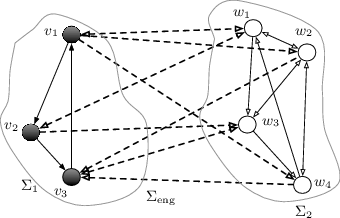
Consider two networks $\Sigma_{1}$ and $\Sigma_{2}$ composed of agents $\{v_{1},\dots,v_{n_{1}}\}$ and agents $\{w_{1},\dots,w_{n_{2}}\}$ , respectively. Throughout this paper, $\Sigma_{1}$ and $\Sigma_{2}$ are either connected undirected graphs, c.f. Section 4, or strongly connected weight-balanced digraphs, c.f. Section 5. Since the latter case includes the first one, throughout this section, we assume the latter. The state of $\Sigma_{1}$ , denoted $x_{1}$ , belongs to $\mathsf{X}_{1}\subset{\mathbb{R}}^{d_{1}}$ , $d_{1}\in\mathbb{Z}_{\geq 1}$ . Likewise, the state of $\Sigma_{2}$ , denoted $x_{2}$ , belongs to $\mathsf{X}_{2}\subset{\mathbb{R}}^{d_{2}}$ , $d_{2}\in\mathbb{Z}_{\geq 1}$ . In this paper, we do not get into the details of what these states represent (as a particular case, the network state could correspond to the collection of the states of agents in it). In addition, each agent $v_{i}$ in $\Sigma_{1}$ has an estimate $x_{1}^{i}\in{\mathbb{R}}^{d_{1}}$ of what the network state is, which may differ from the actual value $x_{1}$ . Similarly, each agent $w_{j}$ in $\Sigma_{2}$ has an estimate $x_{2}^{j}\in{\mathbb{R}}^{d_{2}}$ of what the network state is. Within each network, neighboring agents can share their estimates. Networks can also obtain information about each other. This is modeled by means of a bipartite directed graph $\Sigma_{\textup{eng}}$ , called engagement graph, with disjoint vertex sets $\{v_{1},\ldots,v_{n_{1}}\}$ and $\{w_{1},\ldots,w_{n_{2}}\}$ , where every agent has at least one out-neighbor. According to this model, an agent in $\Sigma_{1}$ obtains information from its out-neighbors in $\Sigma_{\textup{eng}}$ about their estimates of the state of $\Sigma_{2}$ , and vice versa.

Figure 1 illustrates this concept.

Refer to caption — Figure 1: Networks $\Sigma_{1}$ and $\Sigma_{2}$ engaged in a strategic scenario. Both networks are strongly connected and weight-balanced, with weights of $1$ on each edge. Edges which correspond to $\Sigma_{\textup{eng}}$ are dashed.

For each $i\in\{1,\ldots,n_{1}\}$ , let $f_{1}^{i}:\mathsf{X}_{1}\times\mathsf{X}_{2}\rightarrow{\mathbb{R}}$ be a locally Lipschitz concave-convex function only available to agent $v_{i}\in\Sigma_{1}$ . Similarly, let $f_{2}^{j}:\mathsf{X}_{1}\times\mathsf{X}_{2}\rightarrow{\mathbb{R}}$ be a locally Lipschitz concave-convex function only available to agent $w_{j}\in\Sigma_{2}$ , $j\in\{1,\ldots,n_{2}\}$ . The networks $\Sigma_{1}$ and $\Sigma_{2}$ are engaged in a zero-sum game with payoff function $U:\mathsf{X}_{1}\times\mathsf{X}_{2}\rightarrow{\mathbb{R}}$

U(x_{1},x_{2})=\sum_{i=1}^{n_{1}}f_{1}^{i}(x_{1},x_{2})=\sum_{j=1}^{n_{2}}f_{2}^{j}(x_{1},x_{2}),

(3)

where $\Sigma_{1}$ wishes to maximize $U$ , while $\Sigma_{2}$ wishes to minimize it. The objective of the networks is therefore to settle upon a Nash equilibrium, i.e., to solve the following maxmin problem

\max_{x_{1}\in\mathsf{X}_{1}}\min_{x_{2}\in\mathsf{X}_{2}}U(x_{1},x_{2}).

(4)

We refer to the this zero-sum game as the $2$ -network zero-sum game and denote it by $\mathbf{G}_{\textup{adv-net}}=(\Sigma_{1},\Sigma_{2},\Sigma_{\textup{eng}},U)$ . We assume that $\mathsf{X}_{1}\subset{\mathbb{R}}^{d_{1}}$ and $\mathsf{X}_{2}\subset{\mathbb{R}}^{d_{2}}$ are compact convex. For convenience, let $\bm{x}_{1}=(x_{1}^{1},\ldots,x_{1}^{n_{1}})^{T}$ and $\bm{x}_{2}=(x_{2}^{1},\ldots,x_{2}^{n_{2}})^{T}$ denote vector of agent estimates about the state of the respective networks.

Remark 3.1

(Power allocation in communication channels in the presence of adversaries): Here we present an example from communications inspired by (Boyd and Vandenberghe, 2004, Section 5.5.3). Consider $n$ Gaussian communication channels, each with signal power $p_{i}\in{\mathbb{R}}_{\geq 0}$ and noise power $\eta_{i}\in{\mathbb{R}}_{\geq 0}$ , for $i\in\{1,\dots,n\}$ . The capacity of each channel is proportional to $\log(1+\beta p_{i}/(\sigma_{i}+\eta_{i}))$ , where $\beta\in{\mathbb{R}}_{>0}$ and $\sigma_{i}>0$ is the receiver noise. Note that capacity is concave in $p_{i}$ and convex in $\eta_{i}$ . Both signal and noise powers must satisfy a budget constraint, i.e., $\sum_{i=1}^{n}p_{i}=P$ and $\sum_{i=1}^{n}\eta_{i}=C$ , for some given $P,C\in{\mathbb{R}}_{>0}$ . Two networks of $n$ agents are involved in this scenario, one, $\Sigma_{1}$ , selecting signal powers to maximize capacity, the other one, $\Sigma_{2}$ , selecting noise powers to minimize it. The network $\Sigma_{1}$ has decided that $m_{1}$ channels will have signal power $x_{1}$ , while $n-1-m_{1}$ will have signal power $x_{2}$ . The remaining $n$ th channel has its power determined to satisfy the budget constraint, i.e., $P-m_{1}x_{1}-(n-1-m_{1})x_{2}$ . Likewise, the network $\Sigma_{2}$ does something similar with $m_{2}$ channels with noise power $y_{1}$ , $n-1-m_{2}$ channels with noise power $y_{2}$ , and one last channel with noise power $C-m_{2}y_{1}-(n-1-m_{2})y_{2}$ . Each network is aware of the partition made by the other one. The individual objective function of the two agents (one from $\Sigma_{1}$ , the other from $\Sigma_{2}$ ) making decisions on the power levels of the $i$ th channel is the channel capacity itself. For $i\in\{1,\dots,n-1\}$ , this takes the form

\displaystyle f^{i}(x,y)=\log\Big(1+\frac{\beta x_{a}}{\sigma_{i}+y_{b}}\Big),

for some $a,b\in\{1,2\}$ . Here $x=(x_{1},x_{2})$ and $y=(y_{1},y_{2})$ . For $i=n$ , it takes instead the form

\displaystyle f^{n}(x,y)=\log\Big(1+\frac{\beta(P-m_{1}x_{1}-(n-1-m_{1})x_{2})}{\sigma_{n}+C-m_{2}y_{1}-(n-1-m_{2})y_{2}}\Big).

Note that $\sum_{i=1}^{n}f^{i}(x,y)$ is the total capacity of the $n$ communication channels. $\bullet$

3.1 Reformulation of the $2$ -network zero-sum game

In this section, we describe how agents in each network use the information obtained from their neighbors to compute the value of their own objective functions. Based on these estimates, we introduce a reformulation of the $\mathbf{G}_{\textup{adv-net}}=(\Sigma_{1},\Sigma_{2},\Sigma_{\textup{eng}},U)$ which is instrumental for establishing some of our results.

Each agent in $\Sigma_{1}$ has a locally Lipschitz, concave-convex function $\tilde{f}_{1}^{i}:{\mathbb{R}}^{d_{1}}\times{\mathbb{R}}^{d_{2}n_{2}}\rightarrow{\mathbb{R}}$ with the properties:

(Extension of own payoff function):

for any $x_{1}\in{\mathbb{R}}^{d_{1}}$ , $x_{2}\in{\mathbb{R}}^{d_{2}}$ ,

\tilde{f}_{1}^{i}(x_{1},\mathbf{1}_{n_{2}}\otimes x_{2})=f_{1}^{i}(x_{1},x_{2}).

(5a)

(Distributed over $\Sigma_{\textup{eng}}$ ):

there exists $\mathfrak{f}_{1}^{i}:{\mathbb{R}}^{d_{1}}\times{\mathbb{R}}^{d_{2}|\mathcal{N}^{\textup{in}}_{\Sigma_{\textup{eng}}}(v_{i})|}\rightarrow{\mathbb{R}}$ such that, for any $x_{1}\in{\mathbb{R}}^{d_{1}}$ $\bm{x}_{2}\in{\mathbb{R}}^{d_{2}n_{2}}$ ,

\tilde{f}_{1}^{i}(x_{1},\bm{x}_{2})=\mathfrak{f}_{1}^{i}(x_{1},\pi_{1}^{i}(\bm{x}_{2})),

(5b)

with $\pi_{1}^{i}:{\mathbb{R}}^{d_{2}n_{2}}\rightarrow{\mathbb{R}}^{d_{2}|\mathcal{N}^{\textup{out}}_{\Sigma_{\textup{eng}}}(v_{i})|}$ the projection of $\bm{x}_{2}$ to the values received by $v_{i}$ from its out-neighbors in $\Sigma_{\textup{eng}}$ .

Equation (5a) states the fact that, when the estimates of all neighbors of an agent in the opponent’s network agree, its evaluation should coincide with this estimate. Equation (5b) states the fact that agents can only use the information received from their neighbors in the interaction topology to compute their new estimates.

Each agent in $\Sigma_{2}$ has a function $\tilde{f}_{2}^{j}:{\mathbb{R}}^{d_{1}n_{1}}\times{\mathbb{R}}^{d_{2}}\rightarrow{\mathbb{R}}$ with similar properties. The collective payoff functions of the two networks are


$\displaystyle\tilde{U}_{1}(\bm{x}_{1},\bm{x}_{2})$	$\displaystyle=\sum_{i=1}^{n_{1}}\tilde{f}_{1}^{i}(x_{1}^{i},\bm{x}_{2}),$	(6a)
$\displaystyle\tilde{U}_{2}(\bm{x}_{1},\bm{x}_{2})$	$\displaystyle=\sum_{j=1}^{n_{2}}\tilde{f}_{2}^{j}(\bm{x}_{1},x_{2}^{j}).$	(6b)

In general, the functions $\tilde{U}_{1}$ and $\tilde{U}_{2}$ need not be the same. However, $\tilde{U}_{1}(\mathbf{1}_{n_{1}}\otimes x_{1},\mathbf{1}_{n_{1}}\otimes x_{2})=\tilde{U}_{2}(\mathbf{1}_{n_{1}}\otimes x_{1},\mathbf{1}_{n_{1}}\otimes x_{2})$ , for any $x_{1}\in{\mathbb{R}}^{d_{1}}$ , $x_{2}\in{\mathbb{R}}^{d_{2}}$ . When both functions coincide, the next result shows that the original game can be lifted to a (constrained) zero-sum game.

Lemma 3.2

(Reformulation of the $2$ -network zero-sum game): Assume that the individual payoff functions $\{\tilde{f}^{i}_{1}\}_{i=1}^{n_{1}}$ , $\{\tilde{f}^{j}_{2}\}_{j=1}^{n_{2}}$ satisfying (5) are such that the network payoff functions defined in (6) satisfy $\tilde{U}_{1}=\tilde{U}_{2}$ , and let $\tilde{U}$ denote this common function. Then, the problem (4) on ${\mathbb{R}}^{d_{1}}\times{\mathbb{R}}^{d_{2}}$ is equivalent to the following problem on ${\mathbb{R}}^{n_{1}d_{1}}\times{\mathbb{R}}^{n_{2}d_{2}}$ ,

		$\displaystyle\max_{\bm{x}_{1}\in\mathsf{X}_{1}^{n_{1}}}\min_{\bm{x}_{2}\in\mathsf{X}_{2}^{n_{2}}}\tilde{U}(\bm{x}_{1},\bm{x}_{2}),$
		$\displaystyle\qquad\text{subject to}\quad\mathbf{L}_{1}\bm{x}_{1}=\mathbf{0}_{n_{1}d_{1}},\quad\mathbf{L}_{2}\bm{x}_{2}=\mathbf{0}_{n_{2}d_{2}},$		(7)

with $\mathbf{L}_{\ell}=\mathsf{L}_{\ell}\otimes\mathsf{I}_{d_{\ell}}$ and $\mathsf{L}_{\ell}$ the Laplacian of $\Sigma_{\ell}$ , $\ell\in\{1,2\}$ .

Proof.

The proof follows by noting that (i) $\tilde{U}(\mathbf{1}_{n_{1}}\otimes x_{1},\mathbf{1}_{n_{2}}\otimes x_{2})=U(x_{1},x_{2})$ for all $x_{1}\in{\mathbb{R}}^{d_{1}}$ and $x_{2}\in{\mathbb{R}}^{d_{2}}$ and (ii) since $\mathcal{G}_{1}$ and $\mathcal{G}_{2}$ are strongly connected, $\mathbf{L}_{1}\bm{x}_{1}=\mathbf{0}_{n_{1}d_{1}}$ and $\mathbf{L}_{2}\bm{x}_{2}=\mathbf{0}_{n_{2}d_{2}}$ iff $\bm{x}_{1}=\mathbf{1}_{n_{1}}\otimes x_{1}$ and $\bm{x}_{2}=\mathbf{1}_{n_{2}}\otimes x_{2}$ for some $x_{1}\in{\mathbb{R}}^{d_{1}}$ and $x_{2}\in{\mathbb{R}}^{d_{2}}$ . ∎

Remark 3.3

(Restrictions on extensions): The assumption of Lemma 3.2 does not hold in general for all sets of extensions satisfying (5a) and (5b). If the interaction topology is one-to-one (i.e., both networks have the same number of agents, the interaction topology is undirected, and each agent in the first network obtains information only from one agent in the opposing network), the natural extensions satisfy the assumption. Example 5.5 later provides yet another instance of a different nature. In general, determining if it is always possible to choose the extensions in such a way that the assumption holds is an open problem. $\bullet$

We denote by $\mathbf{\tilde{G}}_{\textup{adv-net}}=(\Sigma_{1},\Sigma_{2},\Sigma_{\textup{eng}},\tilde{U})$ the constrained zero-sum game defined by (7) and refer to this situation by saying that $\mathbf{G}_{\textup{adv-net}}$ can be lifted to $\mathbf{\tilde{G}}_{\textup{adv-net}}$ . Our objective is to design a coordination algorithm that is implementable with the information that agents in $\Sigma_{1}$ and $\Sigma_{2}$ possess and leads them to find a Nash equilibrium of $\mathbf{\tilde{G}}_{\textup{adv-net}}$ , which corresponds to a Nash equilibrium of $\mathbf{G}_{\textup{adv-net}}$ by Lemma 3.2. Achieving this goal, however, is nontrivial because individual agents, not networks themselves, are the decision makers. From the point of view of agents in each network, the objective is to agree on the states of both their own network and the other network, and that the resulting states correspond to a Nash equilibrium of $\mathbf{G}_{\textup{adv-net}}$ .

The function $\tilde{U}$ is locally Lipschitz and concave-convex. Moreover, from Lemma 2.2, the elements of $\partial_{\bm{x}_{1}}\tilde{U}(\bm{x}_{1},\bm{x}_{2})$ are of the form

\displaystyle\tilde{g}_{(\bm{x}_{1},\bm{x}_{2})}=(\tilde{g}^{1}_{(x^{1}_{1},\bm{x}_{2})},\ldots,\tilde{g}^{n}_{(x^{n}_{1},\bm{x}_{2})})\in\partial_{\bm{x}_{1}}\tilde{U}(\bm{x}_{1},\bm{x}_{2}),

where $\tilde{g}^{i}_{(x^{i}_{1},\bm{x}_{2})}\in\partial_{x_{1}}\tilde{f}^{i}_{1}(x^{i}_{1},\bm{x}_{2})$ , for $i\in\{1,\ldots,n_{1}\}$ . Note that, because of (5b), we have $\partial_{x_{1}}\tilde{f}^{i}_{1}(x^{i}_{1},\mathbf{1}_{n_{2}}\otimes x_{2})=\partial_{x_{1}}f^{i}_{1}(x^{i}_{1},x_{2})$ . A similar reasoning can be followed to describe the elements of $\partial_{\bm{x}_{2}}\tilde{U}(\bm{x}_{1},\bm{x}_{2})$ . Next, we present a characterization of the Nash equilibria of $\mathbf{\tilde{G}}_{\textup{adv-net}}$ , instrumental for proving some of our upcoming results.

Proposition 3.4

(Characterization of the Nash equilibria of $\mathbf{\tilde{G}}_{\textup{adv-net}}$ ): For $\Sigma_{1}$ , $\Sigma_{2}$ strongly connected and weight-balanced, define $F_{1}$ and $F_{2}$ by

	$\displaystyle F_{1}(\bm{x}_{1},\bm{z}_{1},\bm{x}_{2})$	$\displaystyle=-\tilde{U}(\bm{x}_{1},\bm{x}_{2})+\bm{x}_{1}^{T}\mathbf{L}_{1}\bm{z}_{1}+\frac{1}{2}\bm{x}_{1}^{T}\mathbf{L}_{1}\bm{x}_{1},$
	$\displaystyle F_{2}(\bm{x}_{2},\bm{z}_{2},\bm{x}_{1})$	$\displaystyle=\tilde{U}(\bm{x}_{1},\bm{x}_{2})+\bm{x}_{2}^{T}\mathbf{L}_{2}\bm{z}_{2}+\frac{1}{2}\bm{x}_{2}^{T}\mathbf{L}_{2}\bm{x}_{2}.$

Then, $F_{1}$ and $F_{2}$ are convex in their first argument, linear in their second one, and concave in their third one. Moreover, assume $(\bm{x}^{*}_{1},\bm{z}^{*}_{1},\bm{x}^{*}_{2},\bm{z}^{*}_{2})$ satisfies the following saddle property for $(F_{1},F_{2})$ : $(\bm{x}^{*}_{1},\bm{z}^{*}_{1})$ is a saddle point of $(\bm{x}_{1},\bm{z}_{1})\mapsto F_{1}(\bm{x}_{1},\bm{z}_{1},\bm{x}^{*}_{2})$ and $(\bm{x}^{*}_{2},\bm{z}^{*}_{2})$ is a saddle point of $(\bm{x}_{2},\bm{z}_{2})\mapsto F_{2}(\bm{x}_{2},\bm{z}_{2},\bm{x}^{*}_{1})$ . Then,

(i)

$(\bm{x}^{*}_{1},\bm{z}^{*}_{1}+\mathbf{1}_{n_{1}}\otimes a_{1},\bm{x}^{*}_{2},\bm{z}^{*}_{2}+\mathbf{1}_{n_{2}}\otimes a_{2})$ satisfies the saddle property for $(F_{1},F_{2})$ for any $a_{1}\in{\mathbb{R}}^{d_{1}}$ , $a_{2}\in{\mathbb{R}}^{d_{2}}$ , and
(ii)

$(\bm{x}^{*}_{1},\bm{x}^{*}_{2})$ is a Nash equilibrium of $\mathbf{\tilde{G}}_{\textup{adv-net}}$ .

Furthermore,

(iii)

if $(\bm{x}^{*}_{1},\bm{x}^{*}_{2})$ is a Nash equilibrium of $\mathbf{\tilde{G}}_{\textup{adv-net}}$ then there exists $\bm{z}^{*}_{1},\bm{z}^{*}_{2}$ such that $(\bm{x}^{*}_{1},\bm{z}^{*}_{1},\bm{x}^{*}_{2},\bm{z}^{*}_{2})$ satisfies the saddle property for $(F_{1},F_{2})$ .

Proof.

The statement (i) is immediate. For (ii), since $(\bm{x}^{*}_{1},\bm{z}^{*}_{1},\bm{x}^{*}_{2},\bm{z}^{*}_{2})$ satisfies the saddle property, and the networks are strongly connected and weight-balanced, we have $\bm{x}^{*}_{1}=\mathbf{1}_{n_{1}}\otimes x^{*}_{1}$ , $x^{*}_{1}\in{\mathbb{R}}^{d_{1}}$ , $\bm{x}^{*}_{2}=\mathbf{1}_{n_{2}}\otimes x^{*}_{2}$ , $x^{*}_{2}\in{\mathbb{R}}^{d_{2}}$ , $\mathbf{L}_{1}\bm{z}^{*}_{1}\in-\partial_{\bm{x}_{1}}\tilde{U}(\bm{x}^{*}_{1},\bm{x}^{*}_{2})$ , and $\mathbf{L}_{2}\bm{z}^{*}_{2}\in\partial_{\bm{x}_{2}}\tilde{U}(\bm{x}^{*}_{1},\bm{x}^{*}_{2})$ . Thus there exist $g^{i}_{1,(x^{*}_{1},x^{*}_{2})}\in\partial_{x_{1}}f_{1}^{i}(x^{*}_{1},x^{*}_{2})$ , $i\in\{1,\ldots,n_{1}\}$ , and $g^{j}_{2,(x^{*}_{1},x^{*}_{2})}\in-\partial_{x_{2}}f_{2}^{j}(x^{*}_{1},x^{*}_{2})$ , $j\in\{1,\ldots,n_{2}\}$ , such that

	$\displaystyle\mathbf{L}_{1}\bm{z}_{1}^{*}$	$\displaystyle=(g^{1}_{1,(x^{}_{1},x^{}_{2})},,\ldots,g^{n}_{1,(x^{}_{1},x^{}_{2})}))^{T},\ \mathrm{and}$
	$\displaystyle\mathbf{L}_{2}\bm{z}_{2}^{*}$	$\displaystyle=(g^{1}_{2,(x^{}_{1},x^{}_{2})},,\ldots,g^{n}_{2,(x^{}_{1},x^{}_{2})}))^{T}.$

Noting that, for $\ell\in\{1,2\}$ , $(\mathbf{1}_{n_{\ell}}^{T}\otimes\mathsf{I}_{d_{\ell}})\mathbf{L}_{\ell}=(\mathbf{1}_{n_{\ell}}^{T}\otimes\mathsf{I}_{d_{\ell}})(\mathsf{L}_{\ell}\otimes\mathsf{I}_{d_{\ell}})=\mathbf{1}_{n_{\ell}}^{T}\mathsf{L}\otimes\mathsf{I}_{d_{\ell}}=\mathbf{0}_{d_{\ell}\times d_{\ell}n_{\ell}}$ , we deduce that $\sum_{i=1}^{n_{1}}g^{i}_{1,(x^{*}_{1},x^{*}_{2})}=\mathbf{0}_{d_{1}}$ and $\sum_{j=1}^{n_{2}}g^{j}_{2,(x^{*}_{1},x^{*}_{2})}=\mathbf{0}_{d_{2}}$ , i.e., $(\bm{x}^{*}_{1},\bm{x}^{*}_{2})$ is a Nash equilibrium. Finally for proving (iii), note that $\bm{x}_{1}^{*}=\mathbf{1}_{n_{1}}\otimes x_{1}^{*}$ and $\bm{x}_{2}^{*}=\mathbf{1}_{n_{2}}\otimes x_{2}^{*}$ . The result follows then from the fact that $0\in\partial_{x_{1}}U(x_{1}^{*},x_{2}^{*})$ and $0\in\partial_{x_{2}}U(x_{1}^{*},x_{2}^{*})$ implies that there exists $\bm{z}_{1}^{*}\in{\mathbb{R}}^{n_{1}d_{1}}$ and $\bm{z}_{2}^{*}\in{\mathbb{R}}^{n_{2}d_{2}}$ with $\mathbf{L}_{1}\bm{z}_{1}^{*}\in\partial_{\bm{x}_{1}}\tilde{U}(\bm{x}_{1}^{*},\bm{x}_{2}^{*})$ and $\mathbf{L}_{2}\bm{z}_{2}^{*}\in-\partial_{\bm{x}_{2}}\tilde{U}(\bm{x}_{1}^{*},\bm{x}_{2}^{*})$ . ∎

4 Distributed convergence to Nash equilibria for undirected topologies

In this section, we introduce a distributed dynamics which solves (7) when $\Sigma_{1}$ and $\Sigma_{2}$ are undirected. In particular, we design gradient dynamics to find points with the saddle property for $(F_{1},F_{2})$ prescribed by Proposition 3.4. Consider the set-valued dynamics $\Psi_{\textup{Nash-undir}}:({\mathbb{R}}^{d_{1}n_{1}})^{2}\times({\mathbb{R}}^{d_{2}n_{2}})^{2}\rightrightarrows({\mathbb{R}}^{d_{1}n_{1}})^{2}\times({\mathbb{R}}^{d_{2}n_{2}})^{2}$ ,


$\displaystyle\dot{\bm{x}}_{1}+\mathbf{L}_{1}\bm{x}_{1}+\mathbf{L}_{1}\bm{z}_{1}$	$\displaystyle\in\partial_{\bm{x}_{1}}\tilde{U}(\bm{x}_{1},\bm{x}_{2}),$	(8a)
$\displaystyle\dot{\bm{z}}_{1}$	$\displaystyle=\mathbf{L}_{1}\bm{x}_{1},$	(8b)
$\displaystyle\dot{\bm{x}}_{2}+\mathbf{L}_{2}\bm{x}_{2}+\mathbf{L}_{2}\bm{z}_{2}$	$\displaystyle\in-\partial_{\bm{x}_{2}}\tilde{U}(\bm{x}_{1},\bm{x}_{2}),$	(8c)
$\displaystyle\dot{\bm{z}}_{2}$	$\displaystyle=\mathbf{L}_{2}\bm{x}_{2},$	(8d)

where $\bm{x}_{\ell},\bm{z}_{\ell}\in{\mathbb{R}}^{n_{\ell}d_{\ell}}$ , $\ell\in\{1,2\}$ . Note that (8a)-(8b) and (8c)-(8d) correspond to saddle-point dynamics of $F_{1}$ in $(\bm{x}_{1},\bm{z}_{1})$ and $F_{2}$ in $(\bm{x}_{2},\bm{z}_{2})$ , respectively. Local solutions to this dynamics exist by virtue of Lemmas 2.1 and 2.3. We characterize next its asymptotic convergence properties.

Theorem 4.1

(Distributed convergence to Nash equilibria for undirected networks): Consider the zero-sum game $\mathbf{G}_{\textup{adv-net}}=(\Sigma_{1},\Sigma_{2},\Sigma_{\textup{eng}},U)$ , with $\Sigma_{1}$ and $\Sigma_{2}$ connected undirected graphs, $\mathsf{X}_{1}\subset{\mathbb{R}}^{d_{1}}$ , $\mathsf{X}_{2}\subset{\mathbb{R}}^{d_{2}}$ compact and convex, and $U:\mathsf{X}_{1}\times\mathsf{X}_{2}\rightarrow{\mathbb{R}}$ strictly concave-convex and locally Lipschitz. Assume $\mathbf{G}_{\textup{adv-net}}$ can be lifted to $\mathbf{\tilde{G}}_{\textup{adv-net}}$ . Then, the projection onto the first and third components of the solutions of (8) asymptotically converge to agreement on the Nash equilibrium of $\mathbf{G}_{\textup{adv-net}}$ .

Proof.

Throughout this proof, since property (5b) holds, without loss of generality and for simplicity of notation, we assume that agents in $\Sigma_{1}$ have access to $\bm{x}_{2}$ and, similarly, agents in $\Sigma_{2}$ have access to $\bm{x}_{1}$ . By Theorem 2.5, a solution to (6) exists. By the strict concavity-convexity properties, this solution is, in fact, unique. Let us denote this solution by $\bm{x}_{1}^{*}=\mathbf{1}_{n_{1}}\otimes x^{*}_{1}$ and $\bm{x}_{2}^{*}=\mathbf{1}_{n_{2}}\otimes x^{*}_{2}$ . By Proposition 3.4(iii), there exists $\bm{z}_{1}^{*}$ and $\bm{z}_{2}^{*}$ such that $(\bm{x}_{1}^{*},\bm{z}_{1}^{*},\bm{x}_{2}^{*},\bm{z}_{2}^{*})\in\operatorname{Eq}(\Psi_{\textup{Nash-undir}})$ . First, note that given any initial condition $(\bm{x}^{0}_{1},\bm{z}^{0}_{1},\bm{x}^{0}_{2},\bm{z}^{0}_{2})\in({\mathbb{R}}^{n_{1}d_{1}})^{2}\times({\mathbb{R}}^{n_{2}d_{2}})^{2}$ , the set

	$\displaystyle W_{\bm{z}^{0}_{1},\bm{z}^{0}_{2}}$	$\displaystyle=\{(\bm{x}_{1},\bm{z}_{1},\bm{x}_{2},\bm{z}_{2})\ \|$
		$\displaystyle\ (\mathbf{1}_{n_{\ell}}^{T}\otimes\mathsf{I}_{d_{\ell}})\bm{z}_{\ell}=(\mathbf{1}_{n_{\ell}}^{T}\otimes\mathsf{I}_{d_{\ell}})\bm{z}^{0}_{\ell},\;\ell\in\{1,2\}\}$		(9)

is strongly positively invariant under (8). Consider the function $V:({\mathbb{R}}^{d_{1}n_{1}})^{2}\times({\mathbb{R}}^{d_{2}n_{2}})^{2}\rightarrow{\mathbb{R}}_{\geq 0}$ defined by

	$\displaystyle V($	$\displaystyle\bm{x}_{1},\bm{z}_{1},\bm{x}_{2},\bm{z}_{2})$
		$\displaystyle=\frac{1}{2}(\bm{x}_{1}-\bm{x}_{1}^{})^{T}(\bm{x}_{1}-\bm{x}_{1}^{})+\frac{1}{2}(\bm{z}_{1}-\bm{z}_{1}^{})^{T}(\bm{z}_{1}-\bm{z}_{1}^{})$
		$\displaystyle\quad+\frac{1}{2}(\bm{x}_{2}-\bm{x}_{2}^{})^{T}(\bm{x}_{2}-\bm{x}_{2}^{})+\frac{1}{2}(\bm{z}_{2}-\bm{z}_{2}^{})^{T}(\bm{z}_{2}-\bm{z}_{2}^{}).$

The function $V$ is smooth. Next, we examine its set-valued Lie derivative along $\Psi_{\textup{Nash-undir}}$ . Let $\xi\in\widetilde{\mathcal{L}}_{\Psi_{\textup{Nash-undir}}}V(\bm{x}_{1},\bm{z}_{1},\bm{x}_{2},\bm{z}_{2})$ . By definition, there exists $v\in\Psi_{\textup{Nash-undir}}(\bm{x}_{1},\bm{z}_{1},\bm{x}_{2},\bm{z}_{2})$ , given by

	$\displaystyle v=($	$\displaystyle-\mathbf{L}_{1}\bm{x}_{1}-\mathbf{L}_{1}\bm{z}_{1}+g_{1,(\bm{x}_{1},\bm{x}_{2})},$
		$\displaystyle-\mathbf{L}_{2}\bm{x}_{2}-\mathbf{L}_{2}\bm{z}_{2}-g_{2,(\bm{x}_{1},\bm{x}_{2})},\mathbf{L}_{1}\bm{x}_{1},\mathbf{L}_{2}\bm{x}_{2}),$

where $g_{1,(\bm{x}_{1},\bm{x}_{2})}\in\partial_{\bm{x}_{1}}U(\bm{x}_{1},\bm{x}_{2})$ and $g_{2,(\bm{x}_{1},\bm{x}_{2})}\in\partial_{\bm{x}_{2}}U(\bm{x}_{1},\bm{x}_{2})$ , such that

	$\displaystyle\xi$	$\displaystyle=v\cdot\nabla V(\bm{x}_{1},\bm{z}_{1},\bm{x}_{2},\bm{z}_{2})$
		$\displaystyle=(\bm{x}_{1}-\bm{x}_{1}^{*})^{T}(-\mathbf{L}_{1}\bm{x}_{1}-\mathbf{L}_{1}\bm{z}_{1}+g_{1,(\bm{x}_{1},\bm{x}_{2})})$
		$\displaystyle+(\bm{x}_{2}-\bm{x}_{2}^{*})^{T}(-\mathbf{L}_{2}\bm{x}_{2}-\mathbf{L}_{2}\bm{z}_{2}-g_{2,(\bm{x}_{1},\bm{x}_{2})})$
		$\displaystyle\quad+(\bm{z}_{1}-\bm{z}_{1}^{})^{T}\mathbf{L}_{1}\bm{x}_{1}+(\bm{z}_{2}-\bm{z}_{2}^{})^{T}\mathbf{L}_{2}\bm{x}_{2}.$

Note that $-\mathbf{L}_{1}\bm{x}_{1}-\mathbf{L}_{1}\bm{z}_{1}+g_{1,(\bm{x}_{1},\bm{x}_{2})}\in-\partial_{\bm{x}_{1}}F_{1}(\bm{x}_{1},\bm{z}_{1},\bm{x}_{2})$ , $\mathbf{L}_{1}\bm{x}_{1}\in\partial_{\bm{z}_{1}}F_{1}(\bm{x}_{1},\bm{z}_{1},\bm{x}_{2})$ , $-\mathbf{L}_{2}\bm{x}_{2}-\mathbf{L}_{2}\bm{z}_{2}-g_{2,(\bm{x}_{1},\bm{x}_{2})}\in-\partial_{\bm{x}_{2}}F_{2}(\bm{x}_{1},\bm{z}_{2},\bm{x}_{2})$ , and $\mathbf{L}_{2}\bm{x}_{2}\in\partial_{\bm{z}_{2}}F_{2}(\bm{x}_{2},\bm{z}_{2},\bm{x}_{1})$ . Using the first-order convexity property of $F_{1}$ and $F_{2}$ in their first two arguments, one gets

	$\displaystyle\xi$	$\displaystyle\leq F_{1}(\bm{x}_{1}^{},\bm{z}_{1},\bm{x}_{2})-F_{1}(\bm{x}_{1},\bm{z}_{1},\bm{x}_{2})+F_{2}(\bm{x}_{2}^{},\bm{z}_{2},\bm{x}_{1})$
		$\displaystyle-F_{2}(\bm{x}_{2},\bm{z}_{2},\bm{x}_{1})+F_{1}(\bm{x}_{1},\bm{z}_{1},\bm{x}_{2})-F_{1}(\bm{x}_{1},\bm{z}^{*}_{1},\bm{x}_{2})$
		$\displaystyle+F_{2}(\bm{x}_{2},\bm{z}_{2},\bm{x}_{1})-F_{2}(\bm{x}_{2},\bm{z}_{2}^{*},\bm{x}_{1}).$

Expanding each term and using the fact that $(\bm{x}_{1}^{*},\bm{z}_{1}^{*},\bm{x}_{2}^{*},\bm{z}_{2}^{*})$ $\in\operatorname{Eq}(\Psi_{\textup{Nash-undir}})$ , we simplify this inequality as

	$\displaystyle\xi$	$\displaystyle\leq-\tilde{U}(\bm{x}_{1}^{},\bm{x}_{2})+\tilde{U}(\bm{x}_{1},\bm{x}^{}_{2})-\bm{z}^{*}_{1}\mathbf{L}_{1}\bm{x}_{1}$
		$\displaystyle\quad-\frac{1}{2}\bm{x}_{1}\mathbf{L}_{1}\bm{x}_{1}-\bm{z}^{*}_{2}\mathbf{L}_{2}\bm{x}_{2}-\frac{1}{2}\bm{x}_{2}\mathbf{L}_{2}\bm{x}_{2}.$

By rearranging, we thus have

\displaystyle\xi\leq-F_{2}(\bm{x}_{2},\bm{z}_{2}^{*},\bm{x}_{1}^{*})-F_{1}(\bm{x}_{1},\bm{z}_{1}^{*},\bm{x}_{2}^{*}).

Next, since $F_{2}(\bm{x}_{1}^{*},\bm{z}_{2}^{*},\bm{x}_{2}^{*})+F_{1}(\bm{x}_{2}^{*},\bm{z}_{2}^{*},\bm{x}_{1}^{*})=0$ , we have

	$\displaystyle\xi$	$\displaystyle\leq F_{1}(\bm{x}_{1}^{},\bm{z}_{1}^{},\bm{x}_{2}^{})-F_{1}(\bm{x}_{1},\bm{z}_{1}^{},\bm{x}_{2}^{*})$
		$\displaystyle\quad+F_{2}(\bm{x}_{2}^{},\bm{z}_{2}^{},\bm{x}_{1}^{})-F_{2}(\bm{x}_{2},\bm{z}_{2}^{},\bm{x}^{*}_{1}),$

yielding that $\xi\leq 0$ . As a result,

\max\widetilde{\mathcal{L}}_{\Psi_{\textup{Nash-undir}}}V(\bm{x}_{1},\bm{z}_{1},\bm{x}_{2},\bm{z}_{2})\leq 0.

As a by-product, we conclude that the trajectories of (8) are bounded. By virtue of the set-valued version of the LaSalle Invariance Principle, cf. Theorem 2.4, any trajectory of (8) starting from an initial condition $(\bm{x}_{1}^{0},\bm{z}_{1}^{0},\bm{x}_{2}^{0},\bm{z}_{2}^{0})$ converges to the largest positively invariant set $M$ in $S_{\Psi_{\textup{Nash-undir}},V}\cap V^{-1}(\leq V(\bm{x}_{1}^{0},\bm{z}_{1}^{0},\bm{x}_{2}^{0},\bm{z}_{2}^{0}))$ . Let $(\bm{x}_{1},\bm{z}_{1},\bm{x}_{2},\bm{z}_{2})\in M$ . Because $M\subset S_{\Psi_{\textup{Nash-undir}},V}$ , then $F_{1}(\bm{x}_{1}^{*},\bm{z}_{1}^{*},\bm{x}_{2}^{*})-F_{1}(\bm{x}_{1},\bm{z}_{1}^{*},\bm{x}_{2}^{*})=0,$ i.e.,

-\tilde{U}(\bm{x}_{1}^{*},\bm{x}_{2}^{*})+\tilde{U}(\bm{x}_{1},\bm{x}_{2}^{*})-\bm{x}_{1}^{T}\mathbf{L}_{1}\bm{z}_{1}^{*}-\frac{1}{2}\bm{x}_{1}^{T}\mathbf{L}_{1}\bm{x}_{1}=0.

(10)

Define now $G_{1}:{\mathbb{R}}^{n_{1}d_{1}}\times{\mathbb{R}}^{n_{1}d_{1}}\times{\mathbb{R}}^{n_{2}d_{2}}\rightarrow{\mathbb{R}}$ by $G_{1}(\bm{x}_{1},\bm{z}_{1},\bm{x}_{2})=F_{1}(\bm{x}_{1},\bm{z}_{1},\bm{x}_{2})-\frac{1}{2}\bm{x}_{1}^{T}\mathbf{L}_{1}\bm{x}_{1}$ . $G_{1}$ is convex in its first argument and linear in its second. Furthermore, for fixed $\bm{x}_{2}$ , the map $(\bm{x}_{1},\bm{z}_{1})\mapsto G_{1}(\bm{x}_{1},\bm{z}_{1},\bm{x}_{2})$ has the same saddle points as $(\bm{x}_{1},\bm{z}_{1})\mapsto F_{1}(\bm{x}_{1},\bm{z}_{1},\bm{x}_{2})$ . As a result, $G_{1}(\bm{x}_{1}^{*},\bm{z}_{1}^{*},\bm{x}_{2}^{*})-G_{1}(\bm{x}_{1},\bm{z}^{*}_{1},\bm{x}_{2}^{*})\leq 0$ , or equivalently, $-\tilde{U}(\bm{x}_{1}^{*},\bm{x}_{2}^{*})+\tilde{U}(\bm{x}_{1},\bm{x}_{2}^{*})-\bm{x}_{1}^{T}\mathbf{L}_{1}\bm{z}_{1}^{*}\leq 0$ . Combining this with (10), we have that $\mathbf{L}_{1}\bm{x}_{1}=0$ and $-\tilde{U}(\bm{x}_{1}^{*},\bm{x}_{2}^{*})+\tilde{U}(\bm{x}_{1},\bm{x}_{2}^{*})=0$ . Since $\tilde{U}$ is strictly concave in its first argument $\bm{x}_{1}=\bm{x}_{1}^{*}$ . A similar argument establishes that $\bm{x}_{2}=\bm{x}_{2}^{*}$ . Using now the fact that $M$ is weakly positively invariant, one can deduce that $\mathbf{L}_{\ell}\bm{z}_{\ell}\in-\partial_{\bm{x}_{\ell}}\tilde{U}(\bm{x}_{1},\bm{x}_{2})$ , for $\ell\in\{1,2\}$ , and thus $(\bm{x}_{1},\bm{z}_{1},\bm{x}_{2},\bm{z}_{2})\in\operatorname{Eq}(\Psi_{\textup{Nash-undir}})$ . ∎

5 Distributed convergence to Nash equilibria for directed topologies

Interestingly, the saddle-point dynamics (8) fails to converge when transcribed to the directed network setting. This observation is a consequence of the following result, which studies the stability of the linearization of the dynamics (8), when the payoff functions have no contribution to the linear part.

Lemma 5.1

(Necessary condition for the convergence of (8) on digraphs): Let $\Sigma_{\ell}$ be strongly connected and $f^{i}_{\ell}=0$ , $i\in\{1,\ldots,n_{\ell}\}$ , for $\ell\in\{1,2\}$ . Then, the set of network agreement configurations $\mathcal{S}_{\text{agree}}=\{(\mathbf{1}_{n_{1}}\otimes x_{1},\mathbf{1}_{n_{1}}\otimes z_{1},\mathbf{1}_{n_{2}}\otimes x_{2},\mathbf{1}_{n_{2}}\otimes z_{2})\in({\mathbb{R}}^{n_{1}d_{1}})^{2}\times({\mathbb{R}}^{n_{2}d_{2}})^{2}\;|\;x_{\ell},z_{\ell}\in{\mathbb{R}}^{d_{\ell}},\ell\in\{1,2\}\}$ , is stable under (8) iff, for any nonzero eigenvalue $\lambda$ of the Laplacian $\mathsf{L}_{\ell}$ , $\ell\in\{1,2\}$ , one has $\sqrt{3}|\mathrm{Im}(\lambda)|\leq\mathrm{Re}(\lambda)$ .

Proof.

In this case, (8) is linear with matrix

\displaystyle\begin{pmatrix}\left(\begin{smallmatrix}-1&-1\\ 1&0\end{smallmatrix}\right)\otimes\mathbf{L}_{1}&0\\ 0&\left(\begin{smallmatrix}-1&-1\\ 1&0\end{smallmatrix}\right)\otimes\mathbf{L}_{2}\end{pmatrix}

(11)

and has $\mathcal{S}_{\text{agree}}$ as equilibria. The eigenvalues of (11) are of the form $\lambda_{\ell}\,\big(\frac{-1}{2}\pm\frac{\sqrt{3}}{2}i\big)$ , with $\lambda_{\ell}$ an eigenvalue of $\mathbf{L}_{\ell}$ , for $\ell\in\{1,2\}$ (since the eigenvalues of a Kronecker product are the product of the eigenvalues of the corresponding matrices). Since $\mathbf{L}_{\ell}=\mathsf{L}_{\ell}\otimes\mathsf{I}_{d_{\ell}}$ , each eigenvalue of $\mathbf{L}_{\ell}$ is an eigenvalue of $\mathsf{L}_{\ell}$ . The result follows by noting that $\mathrm{Re}\big(\lambda_{\ell}\big(\frac{-1}{2}\pm\frac{\sqrt{3}}{2}i\big)\big)=\frac{1}{2}(\mp\sqrt{3}\mathrm{Im}(\lambda_{\ell})-\mathrm{Re}(\lambda_{\ell}))$ .∎

It is not difficult to construct examples of strictly concave-convex functions that have zero contribution to the linearization of (8) around the solution. Therefore, such systems cannot be convergent if they fail the necessary condition identified in Lemma 5.1. The counterexample provided in our recent paper (Gharesifard and Cortés, 2012c) of strongly connected, weight-balanced digraphs that do not meet the stability criterium of Lemma 5.1 is therefore valid in this context too.

From here on, we assume that the payoff functions are differentiable. We elaborate on the reasons for this assumption in Remark 5.3 later. Motivated by the observation made in Lemma 5.1, we introduce a parameter $\alpha\in{\mathbb{R}}_{>0}$ in the dynamics of (8) as


$\displaystyle\dot{\bm{x}}_{1}+\alpha\mathbf{L}_{1}\bm{x}_{1}+\mathbf{L}_{1}\bm{z}_{1}$	$\displaystyle=\nabla\tilde{U}(\bm{x}_{1},\bm{x}_{2}),$	(12a)
$\displaystyle\dot{\bm{z}}_{1}$	$\displaystyle=\mathbf{L}_{1}\bm{x}_{1},$	(12b)
$\displaystyle\dot{\bm{x}}_{2}+\alpha\mathbf{L}_{2}\bm{x}_{2}+\mathbf{L}_{2}s\bm{z}_{2}$	$\displaystyle=-\nabla\tilde{U}(\bm{x}_{1},\bm{x}_{2}),$	(12c)
$\displaystyle\dot{\bm{z}}_{2}$	$\displaystyle=\mathbf{L}_{2}\bm{x}_{2}.$	(12d)

We next show that a suitable choice of $\alpha$ makes the dynamics convergent to the Nash equilibrium.

Theorem 5.2

(Distributed convergence to Nash equilibria for directed networks): Consider the zero-sum game $\mathbf{G}_{\textup{adv-net}}=(\Sigma_{1},\Sigma_{2},\Sigma_{\textup{eng}},U)$ , with $\Sigma_{1}$ and $\Sigma_{2}$ strongly connected and weight-balanced digraphs, $\mathsf{X}_{1}\subset{\mathbb{R}}^{d_{1}}$ , $\mathsf{X}_{2}\subset{\mathbb{R}}^{d_{2}}$ compact and convex, and $U:\mathsf{X}_{1}\times\mathsf{X}_{2}\rightarrow{\mathbb{R}}$ strictly concave-convex and differentiable with globally Lipschitz gradient. Assume $\mathbf{G}_{\textup{adv-net}}$ can be lifted to $\mathbf{\tilde{G}}_{\textup{adv-net}}$ such that $\tilde{U}$ is differentiable and has a globally Lipschitz gradient. Define $h:{\mathbb{R}}_{>0}\rightarrow{\mathbb{R}}$ by

	$\displaystyle h(r)=$	$\displaystyle\frac{1}{2}\Lambda_{*}^{\min}\Big(\sqrt{\Big(\frac{r^{4}+3r^{2}+2}{r}\Big)^{2}-4}-\frac{r^{4}+3r^{2}+2}{r}\Big)$
		$\displaystyle+\frac{Kr^{2}}{(1+r^{2})},$		(13)

where $\Lambda_{*}^{\min}=\min_{\ell=1,2}\{\Lambda_{*}(\mathsf{L}_{\ell}+\mathsf{L}_{\ell}^{T})\}$ , $\Lambda_{*}(\cdot)$ denotes the smallest non-zero eigenvalue and $K\in{\mathbb{R}}_{>0}$ is the Lipschitz constant of the gradient of $\tilde{U}$ . Then there exists $\beta^{*}\in{\mathbb{R}}_{>0}$ with $h(\beta^{*})=0$ such that for all $0<\beta<\beta^{*}$ , the projection onto the first and third components of the solutions of (12) with $\alpha=\frac{\beta^{2}+2}{\beta}$ asymptotically converge to agreement on the Nash equilibrium of $\mathbf{G}_{\textup{adv-net}}$ .

Proof.

Similarly to the proof of Theorem 4.1, we assume, without loss of generality, that agents in $\Sigma_{1}$ have access to $\bm{x}_{2}$ and agents in $\Sigma_{2}$ to $\bm{x}_{1}$ . For convenience, we denote the dynamics described in (12) by $\Psi_{\textup{Nash-dir}}:({\mathbb{R}}^{d_{1}n_{1}})^{2}\times({\mathbb{R}}^{d_{2}n_{2}})^{2}\rightarrow({\mathbb{R}}^{d_{1}n_{1}})^{2}\times({\mathbb{R}}^{d_{2}n_{2}})^{2}$ . Let $(\bm{x}_{1}^{0},\bm{z}_{1}^{0},\bm{x}_{2}^{0},\bm{z}_{2}^{0})$ be an arbitrary initial condition. Note that the set $W_{\bm{z}^{0}_{1},\bm{z}^{0}_{2}}$ defined by (9) is invariant under the evolutions of (12). By an argument similar to the one in the proof of Theorem 4.1, there exists a unique solution to (7), which we denote by $\bm{x}_{1}^{*}=\mathbf{1}_{n_{1}}\otimes x^{*}_{1}$ and $\bm{x}_{2}^{*}=\mathbf{1}_{n_{2}}\otimes x^{*}_{2}$ . By Proposition 3.4(i), there exists $(\bm{x}^{*}_{1},\bm{z}^{*}_{1},\bm{x}^{*}_{2},\bm{z}^{*}_{2})\in\operatorname{Eq}(\Psi_{\textup{Nash-dir}})\cap W_{\bm{z}^{0}_{1},\bm{z}^{0}_{2}}$ . Consider the function $V:({\mathbb{R}}^{d_{1}n_{1}})^{2}\times({\mathbb{R}}^{d_{2}n_{2}})^{2}\rightarrow{\mathbb{R}}_{\geq 0}$ ,

	$\displaystyle V(\bm{x}_{1}$	$\displaystyle,\bm{z}_{1},\bm{x}_{2},\bm{z}_{2})$
		$\displaystyle=\frac{1}{2}(\bm{x}_{1}-\bm{x}^{}_{1})^{T}(\bm{x}_{1}-\bm{x}^{}_{1})+\frac{1}{2}(\bm{x}_{2}-\bm{x}^{}_{2})^{T}(\bm{x}_{2}-\bm{x}^{}_{2})$
		$\displaystyle\quad+\frac{1}{2}(\bm{y}_{(\bm{x}_{1},\bm{z}_{1})}-\bm{y}_{(\bm{x}^{}_{1},\bm{z}^{}_{1})})^{T}(\bm{y}_{(\bm{x}_{1},\bm{z}_{1})}-\bm{y}_{(\bm{x}^{}_{1},\bm{z}^{}_{1})}),$
		$\displaystyle\quad+\frac{1}{2}(\bm{y}_{(\bm{x}_{2},\bm{z}_{2})}-\bm{y}_{(\bm{x}^{}_{2},\bm{z}^{}_{2})})^{T}(\bm{y}_{(\bm{x}_{2},\bm{z}_{2})}-\bm{y}_{(\bm{x}^{}_{2},\bm{z}^{}_{2})}),$

where $\bm{y}_{(\bm{x}_{\ell},\bm{z}_{\ell})}=\beta\bm{x}_{\ell}+\bm{z}_{\ell}$ , $\ell\in\{1,2\}$ , and $\beta\in{\mathbb{R}}_{>0}$ satisfies $\beta^{2}-\alpha\beta+2=0$ . This function is quadratic, hence smooth. Next, we consider $\xi=\mathcal{L}_{\Psi_{\textup{Nash-dir}}}V(\bm{x}_{1},\bm{z}_{1},\bm{x}_{2},\bm{z}_{2})$ given by

	$\displaystyle\xi$	$\displaystyle=(-\alpha\mathbf{L}_{1}\bm{x}_{1}-\mathbf{L}_{1}\bm{z}_{1}+\nabla\tilde{U}(\bm{x}_{1},\bm{x}_{2}),\mathbf{L}_{1}\bm{x}_{1},-\alpha\mathbf{L}_{2}\bm{x}_{2}$
		$\displaystyle\quad-\mathbf{L}_{2}\bm{z}_{2}-\nabla\tilde{U}(\bm{x}_{1},\bm{x}_{2}),\mathbf{L}_{2}\bm{x}_{2})\cdot\nabla V(\bm{x}_{1},\bm{z}_{1},\bm{x}_{2},\bm{z}_{2}).$

After some manipulation, one can show that

	$\displaystyle\xi$	$\displaystyle=\sum_{\ell=1}^{2}\frac{1}{2}(\bm{x}_{\ell}-\bm{x}^{}_{\ell},\bm{y}_{(\bm{x}_{\ell},\bm{z}_{\ell})}-\bm{y}_{(\bm{x}^{}_{\ell},\bm{z}^{*}_{\ell})})^{T}A_{\ell}(\bm{x}_{l},\bm{y}_{(\bm{x}_{\ell},\bm{z}_{\ell})})$
		$\displaystyle+\sum_{\ell=1}^{2}\frac{1}{2}(\bm{x}_{\ell}^{T},\bm{y}_{(\bm{x}_{\ell},\bm{z}_{\ell})}^{T})A_{\ell}^{T}(\bm{x}_{\ell}-\bm{x}^{}_{\ell},\bm{y}_{(\bm{x}_{\ell},\bm{z}_{\ell})}-\bm{y}_{(\bm{x}^{}_{\ell},\bm{z}^{*}_{\ell})})$
		$\displaystyle+\sum_{\ell=1}^{2}(-1)^{j-1}(\bm{x}_{\ell}-\bm{x}^{*}_{\ell})^{T}\nabla_{\bm{x}_{\ell}}\tilde{U}(\bm{x}_{1},\bm{x}_{2})$
		$\displaystyle+\sum_{\ell=1}^{2}(-1)^{j-1}\beta(\bm{y}_{(\bm{x}_{\ell},\bm{z}_{\ell})}-\bm{y}_{(\bm{x}^{}_{\ell},\bm{z}^{}_{\ell})})^{T}\nabla_{\bm{x}_{\ell}}\tilde{U}(\bm{x}_{1},\bm{x}_{2}),$

where $A_{\ell}$ , $\ell\in\{1,2\}$ , is

A_{\ell}=\begin{pmatrix}-(\alpha-\beta)\mathbf{L}_{\ell}&-\mathbf{L}_{\ell}\\ (-\beta(\alpha-\beta)+1)\mathbf{L}_{\ell}&-\beta\mathbf{L}_{\ell}\end{pmatrix}.

This equation can be written as

	$\displaystyle\xi$	$\displaystyle=\sum_{\ell=1}^{2}\frac{1}{2}(\bm{x}_{\ell}-\bm{x}^{}_{\ell},\bm{y}_{(\bm{x}_{\ell},\bm{z}_{\ell})}-\bm{y}_{(\bm{x}^{}_{\ell},\bm{z}^{*}_{\ell})})^{T}$
		$\displaystyle\qquad\qquad Q_{\ell}(\bm{x}_{\ell}-\bm{x}^{}_{\ell},\bm{y}_{(\bm{x}_{\ell},\bm{z}_{\ell})}-\bm{y}_{(\bm{x}^{}_{\ell},\bm{z}^{*}_{\ell})})$
		$\displaystyle+\sum_{\ell=1}^{2}(\bm{x}_{\ell}-\bm{x}^{}_{\ell},\bm{y}_{(\bm{x}_{\ell},\bm{z}_{\ell})}-\bm{y}_{(\bm{x}^{}_{\ell},\bm{z}^{}_{\ell})})^{T}A_{\ell}(\bm{x}^{}_{\ell},\bm{y}_{(\bm{x}^{}_{\ell},\bm{z}^{}_{\ell})})$
		$\displaystyle+\sum_{\ell=1}^{2}(-1)^{j-1}(\bm{x}_{\ell}-\bm{x}^{*}_{\ell})^{T}\nabla_{\bm{x}_{\ell}}\tilde{U}(\bm{x}_{1},\bm{x}_{2})$
		$\displaystyle+\sum_{\ell=1}^{2}(-1)^{j-1}\beta(\bm{y}_{(\bm{x}_{\ell},\bm{z}_{\ell})}-\bm{y}_{(\bm{x}^{}_{\ell},\bm{z}^{}_{\ell})})^{T}\nabla_{\bm{x}_{\ell}}\tilde{U}(\bm{x}_{1},\bm{x}_{2}),$

where $Q_{\ell}$ , $\ell\in\{1,2\}$ , is given by

Q_{\ell}=(\mathbf{L}_{\ell}+\mathbf{L}_{\ell}^{T})\otimes\begin{pmatrix}-(\frac{\beta^{2}+2}{\beta}-\beta)&-1\\ -1&-\beta\end{pmatrix}.

(14)

Note that, we have

	$\displaystyle A_{1}(\bm{x}^{}_{1},\bm{y}_{(\bm{x}^{}_{1},\bm{z}^{*}_{1})})$	$\displaystyle=-(\mathbf{L}_{1}\bm{y}_{(\bm{x}^{}_{1},\bm{z}^{}_{1})},\beta\mathbf{L}_{1}\bm{y}_{(\bm{x}^{}_{1},\bm{z}^{}_{1})})$
		$\displaystyle=-(\nabla_{\bm{x}_{1}}\tilde{U}(\bm{x}^{}_{1},\bm{x}_{2}),\beta\nabla_{\bm{x}_{1}}\tilde{U}(\bm{x}^{}_{1},\bm{x}_{2})),$
	$\displaystyle A_{2}(\bm{x}^{}_{2},\bm{y}_{(\bm{x}^{}_{2},\bm{z}^{*}_{2})})$	$\displaystyle=-(\mathbf{L}_{2}\bm{y}_{(\bm{x}^{}_{2},\bm{z}^{}_{2})},\beta\mathbf{L}_{2}\bm{y}_{(\bm{x}^{}_{2},\bm{z}^{}_{2})})$
		$\displaystyle=(\nabla_{\bm{x}_{2}}\tilde{U}(\bm{x}_{1},\bm{x}^{}_{2}),\beta\nabla_{\bm{x}_{2}}\tilde{U}(\bm{x}_{1},\bm{x}^{}_{2})).$

Thus, after substituting for $\bm{y}_{(\bm{x}_{\ell},\bm{z}_{\ell})}$ , we have

		$\displaystyle\xi=\sum_{\ell=1}^{2}\frac{1}{2}(\bm{x}_{\ell}-\bm{x}^{}_{\ell},\bm{z}_{\ell}-\bm{z}^{}_{\ell})^{T}\tilde{Q}_{\ell}(\bm{x}_{\ell}-\bm{x}^{}_{\ell},\bm{z}_{\ell}-\bm{z}^{}_{\ell})$
		$\displaystyle\;+(1+\beta^{2})(\bm{x}_{1}-\bm{x}^{}_{1})^{T}(\nabla_{\bm{x}_{1}}\tilde{U}(\bm{x}_{1},\bm{x}_{2})-\nabla_{\bm{x}_{1}}\tilde{U}(\bm{x}^{}_{1},\bm{x}_{2}))$
		$\displaystyle\;-(1+\beta^{2})(\bm{x}_{2}-\bm{x}^{}_{2})^{T}(\nabla_{\bm{x}_{2}}\tilde{U}(\bm{x}_{1},\bm{x}_{2})-\nabla_{\bm{x}_{2}}\tilde{U}(\bm{x}_{1},\bm{x}^{}_{2}))$
		$\displaystyle\;+\beta(\bm{z}_{1}-\bm{z}^{}_{1})^{T}(\nabla_{\bm{x}_{1}}\tilde{U}(\bm{x}_{1},\bm{x}_{2})-\nabla_{\bm{x}_{1}}\tilde{U}(\bm{x}^{}_{1},\bm{x}_{2}))$
		$\displaystyle\;-\beta(\bm{z}_{2}-\bm{z}^{}_{2})^{T}(\nabla_{\bm{x}_{2}}\tilde{U}(\bm{x}_{1},\bm{x}_{2})-\nabla_{\bm{x}_{2}}\tilde{U}(\bm{x}_{1},\bm{x}^{}_{2})),$		(15)

where

\displaystyle\tilde{Q}_{\ell}=\begin{pmatrix}-\beta^{3}-(\frac{\beta^{2}+2}{\beta})-\beta&-(1+\beta^{2})\\ -(1+\beta^{2})&-\beta\\ \end{pmatrix}\otimes(\mathbf{L}_{\ell}+\mathbf{L}_{\ell}^{T}),

for $\ell\in\{1,2\}$ . Each eigenvalue of $\tilde{Q}_{\ell}$ is of the form

\displaystyle\tilde{\eta}_{\ell}=\lambda_{\ell}\frac{-(\beta^{4}+3\beta^{2}+2)\pm\sqrt{(\beta^{4}+3\beta^{2}+2)^{2}-4\beta^{2}}}{2\beta},

(16)

where $\lambda_{\ell}$ is an eigenvalue of $\mathsf{L}_{\ell}+\mathsf{L}_{\ell}^{T}$ , $\ell\in\{1,2\}$ . Using now Theorem A.1 twice, one for $(\bm{x}_{1},\bm{x}_{2})$ , $(\bm{x}_{1}^{*},\bm{x}_{2})$ , and another one for $(\bm{x}_{1},\bm{x}_{2})$ , $(\bm{x}_{1},\bm{x}_{2}^{*})$ , we have

		$\displaystyle(\bm{x}_{1}-\bm{x}^{}_{1})^{T}(\nabla_{\bm{x}_{1}}\tilde{U}(\bm{x}_{1},\bm{x}_{2})-\nabla_{\bm{x}_{1}}\tilde{U}(\bm{x}^{}_{1},\bm{x}_{2}))\leq$
		$\displaystyle\quad-\frac{1}{K}\left(\|\|\nabla_{\bm{x}_{1}}\tilde{U}(\bm{x}_{1},\bm{x}_{2})-\nabla_{\bm{x}_{1}}\tilde{U}(\bm{x}^{*}_{1},\bm{x}_{2})\|\|^{2}\right),$
	$\displaystyle-$	$\displaystyle(\bm{x}_{2}-\bm{x}^{}_{2})^{T}(\nabla_{\bm{x}_{2}}\tilde{U}(\bm{x}_{1},\bm{x}_{2})-\nabla_{\bm{x}_{2}}\tilde{U}(\bm{x}_{1},\bm{x}_{2}^{}))\leq$
		$\displaystyle\quad-\frac{1}{K}\left(\|\|\nabla_{\bm{x}_{2}}\tilde{U}(\bm{x}_{1},\bm{x}_{2})-\nabla_{\bm{x}_{2}}\tilde{U}(\bm{x}_{1},\bm{x}^{*}_{2})\|\|^{2}\right),$

where $K\in{\mathbb{R}}_{>0}$ is the Lipschitz constant of $\nabla\tilde{U}$ . We thus conclude that

		$\displaystyle\xi\leq\sum_{\ell=1}^{2}\frac{1}{2}(\bm{x}_{\ell}-\bm{x}^{}_{\ell},\bm{z}_{\ell}-\bm{z}^{}_{\ell})^{T}\tilde{Q}_{\ell}(\bm{x}_{\ell}-\bm{x}^{}_{\ell},\bm{z}_{\ell}-\bm{z}^{}_{\ell})$
		$\displaystyle-\frac{(1+\beta^{2})}{K}\big(\|\|\nabla_{\bm{x}_{1}}\tilde{U}(\bm{x}_{1},\bm{x}_{2})-\nabla_{\bm{x}_{1}}\tilde{U}(\bm{x}^{*}_{1},\bm{x}_{2})\|\|^{2}$
		$\displaystyle+\|\|\nabla_{\bm{x}_{2}}\tilde{U}(\bm{x}_{1},\bm{x}_{2})-\nabla_{\bm{x}_{2}}\tilde{U}(\bm{x}_{1},\bm{x}^{*}_{2})\|\|^{2}\big)$
		$\displaystyle+\beta(\bm{z}_{1}-\bm{z}^{}_{1})^{T}(\nabla_{\bm{x}_{1}}\tilde{U}(\bm{x}_{1},\bm{x}_{2})-\nabla_{\bm{x}_{1}}\tilde{U}(\bm{x}^{}_{1},\bm{x}_{2}))$
		$\displaystyle-\beta(\bm{z}_{2}-\bm{z}^{}_{2})^{T}(\nabla_{\bm{x}_{2}}\tilde{U}(\bm{x}_{1},\bm{x}_{2})-\nabla_{\bm{x}_{2}}\tilde{U}(\bm{x}_{1},\bm{x}^{}_{2})).$

One can write this inequality as displayed in (17),

\displaystyle\xi\leq\frac{1}{2}X^{T}\underbrace{\begin{pmatrix}Q_{1,11}&Q_{1,12}&0&0&0&0\\ Q_{1,21}&Q_{1,22}&0&0&\beta\mathsf{I}_{n_{1}d_{1}}&0\\ 0&0&Q_{2,11}&Q_{2,12}&0&0\\ 0&0&Q_{2,21}&Q_{2,22}&0&-\beta\mathsf{I}_{n_{2}d_{2}}\\ 0&\beta\mathsf{I}_{n_{1}d_{1}}&0&0&-\tfrac{(1+\beta^{2})}{K}\mathsf{I}_{n_{1}d_{1}}&0\\ 0&0&0&-\beta\mathsf{I}_{n_{2}d_{2}}&0&-\tfrac{(1+\beta^{2})}{K}\mathsf{I}_{n_{2}d_{2}}\end{pmatrix}}_{\mathbf{Q}}X,

(17)

where

	$\displaystyle X=($	$\displaystyle\bm{x}_{1}-\bm{x}^{}_{1},\bm{z}_{1}-\bm{z}^{}_{1},\bm{x}_{2}-\bm{x}^{}_{2},\bm{z}_{2}-\bm{z}^{}_{2},$
		$\displaystyle\nabla_{\bm{x}_{1}}\tilde{U}(\bm{x}_{1},\bm{x}_{2})-\nabla_{\bm{x}_{1}}\tilde{U}(\bm{x}^{*}_{1},\bm{x}_{2}),$
		$\displaystyle\nabla_{\bm{x}_{2}}\tilde{U}(\bm{x}_{1},\bm{x}_{2})-\nabla_{\bm{x}_{2}}\tilde{U}(\bm{x}_{1},\bm{x}^{*}_{2})).$

Since $(\bm{x}_{1},\bm{z}_{1},\bm{x}_{2},\bm{z}_{2})\in W_{\bm{z}^{0}_{1},\bm{z}^{0}_{2}}$ , we have $(\mathbf{1}_{n_{\ell}}^{T}\otimes\mathsf{I}_{d_{\ell}})(\bm{z}_{\ell}-\bm{z}_{\ell}^{*})=\mathbf{0}_{d_{\ell}}$ , $\ell\in\{1,2\}$ , and hence it is enough to establish that $\mathbf{Q}$ is negative semidefinite on the subspace $\mathcal{W}=\{(v_{1},v_{2},v_{3},v_{4},v_{5},v_{6})\in({\mathbb{R}}^{n_{1}d_{1}})^{2}\times({\mathbb{R}}^{n_{2}d_{2}})^{2}\times{\mathbb{R}}^{n_{1}d_{1}}\times{\mathbb{R}}^{n_{2}d_{2}}\;|\;(\mathbf{1}_{n_{1}}^{T}\otimes\mathsf{I}_{d_{1}})v_{2}=\mathbf{0}_{d_{1}},(\mathbf{1}_{n_{2}}^{T}\otimes\mathsf{I}_{d_{2}})v_{4}=\mathbf{0}_{n_{2}}\}$ . Using the fact that $-\tfrac{1}{K}(1+\beta^{2})\mathsf{I}_{n_{\ell}d_{\ell}}$ is invertible, for $\ell\in\{1,2\}$ , we can express $\mathbf{Q}$ as

		$\displaystyle\mathbf{Q}=$
		$\displaystyle\ N\underbrace{\begin{pmatrix}\bar{Q}_{1}&0&0&0\\ 0&\bar{Q}_{2}&0&0\\ 0&0&-\tfrac{1}{K}(1+\beta^{2})\mathsf{I}_{n_{1}d_{1}}&0\\ 0&0&0&-\tfrac{1}{K}(1+\beta^{2})\mathsf{I}_{n_{2}d_{2}}\\ \end{pmatrix}}_{\mathbf{D}}N^{T},$

where $\bar{Q}_{\ell}=\tilde{Q}_{\ell}+\frac{K\beta^{2}}{(1+\beta^{2})}\left(\begin{matrix}0&0\\ 0&\mathsf{I}_{n_{\ell}d_{\ell}}\end{matrix}\right)$ , $\ell\in\{1,2\}$ , and

\displaystyle N=\begin{pmatrix}\mathsf{I}_{n_{1}d_{1}}&0&0&0&0&0\\ 0&\mathsf{I}_{n_{1}d_{1}}&0&0&-\frac{\beta K}{1+\beta^{2}}\mathsf{I}_{n_{1}d_{1}}&0\\ 0&0&\mathsf{I}_{n_{2}d_{2}}&0&0&0\\ 0&0&0&\mathsf{I}_{n_{2}d_{2}}&0&\frac{\beta K}{1+\beta^{2}}\mathsf{I}_{n_{2}d_{2}}\\ 0&0&0&0&\mathsf{I}_{n_{1}d_{1}}&0\\ 0&0&0&0&0&\mathsf{I}_{n_{2}d_{2}}\\ \end{pmatrix}.

Noting that $\mathcal{W}$ is invariant under $N^{T}$ (i.e., $N^{T}\mathcal{W}=\mathcal{W}$ ), all we need to check is that the matrix $\mathbf{D}$ is negative semidefinite on $\mathcal{W}$ . Clearly,

\displaystyle\left(\begin{smallmatrix}-\tfrac{1}{K}(1+\beta^{2})\mathsf{I}_{n_{1}d_{1}}&0\\ 0&-\tfrac{1}{K}(1+\beta^{2})\mathsf{I}_{n_{2}d_{2}}\end{smallmatrix}\right)

is negative definite. On the other hand, for $\ell\in\{1,2\}$ , on $({\mathbb{R}}^{n_{\ell}d_{\ell}})^{2}$ , $0$ is an eigenvalue of $\tilde{Q}_{\ell}$ with multiplicity $2d_{\ell}$ and eigenspace generated by vectors of the form $(\mathbf{1}_{n_{\ell}}\otimes a,0)$ and $(0,\mathbf{1}_{n_{\ell}}\otimes b)$ , with $a,b\in{\mathbb{R}}^{d_{\ell}}$ . However, on $\{(v_{1},v_{2})\in({\mathbb{R}}^{n_{\ell}d_{\ell}})^{2}\;|\;(\mathbf{1}_{n_{\ell}}^{T}\otimes\mathsf{I}_{d_{\ell}})v_{2}=\mathbf{0}_{d_{\ell}}\}$ , $0$ is an eigenvalue of $\tilde{Q}_{\ell}$ with multiplicity $d_{\ell}$ and eigenspace generated by vectors of the form $(\mathbf{1}_{n_{\ell}}\otimes a,0)$ . Moreover, on $\{(v_{1},v_{2})\in({\mathbb{R}}^{n_{\ell}d_{\ell}})^{2}\;|\;(\mathbf{1}_{n_{\ell}}^{T}\otimes\mathsf{I}_{d_{\ell}})v_{2}=\mathbf{0}_{d_{\ell}}\}$ , the eigenvalues of $\frac{K\beta^{2}}{(1+\beta^{2})}\left(\begin{smallmatrix}0&0\\ 0&\mathsf{I}_{n_{\ell}d_{\ell}}\end{smallmatrix}\right)$ are $\frac{K\beta^{2}}{(1+\beta^{2})}$ with multiplicity $n_{\ell}d_{\ell}-d_{\ell}$ and $0$ with multiplicity $n_{\ell}d_{\ell}$ . Therefore, using Weyl’s theorem (Horn and Johnson, 1985, Theorem 4.3.7), we deduce that the nonzero eigenvalues of the sum $\bar{Q}_{\ell}$ are upper bounded by $\Lambda_{*}(\tilde{Q}_{\ell})+\frac{K\beta^{2}}{(1+\beta^{2})}$ . Thus, the eigenvalues of $\bar{Q}=\left(\begin{smallmatrix}\bar{Q}_{1}&0\\ 0&\bar{Q}_{2}\end{smallmatrix}\right)$ are upper bounded by $\min_{\ell=1,2}\{\Lambda_{*}(\bar{Q}_{\ell})\}+\frac{K\beta^{2}}{(1+\beta^{2})}$ . From (16) and the definition of $h$ in (13), we conclude that the nonzero eigenvalues of $\bar{Q}$ are upper bounded by $h(\beta)$ . It remains to show that there exists $\beta^{*}\in{\mathbb{R}}_{>0}$ with $h(\beta^{*})=0$ such that for all $0<\beta<\beta^{*}$ we have $h(\beta)<0$ . For $r>0$ small enough, $h(r)<0$ , since $h(r)=-\frac{1}{2}\Lambda_{*}^{\min}r+O(r^{2})$ . Furthermore, $\lim_{r\rightarrow\infty}h(r)=K>0$ . Hence, using the Mean Value Theorem, we deduce the existence of $\beta^{*}$ . Therefore we conclude that $\mathcal{L}_{\Psi_{\textup{Nash-dir}}}V(\bm{x}_{1},\bm{z}_{1},\bm{x}_{2},\bm{z}_{2})\leq 0$ . As a by-product, the trajectories of (8) are bounded. Consequently, all assumptions of the LaSalle Invariance Principle, cf. Theorem 2.4, are satisfied. This result then implies that any trajectory of (8) starting from an initial condition $(\bm{x}_{1}^{0},\bm{z}_{1}^{0},\bm{x}_{2}^{0},\bm{z}_{2}^{0})$ converges to the largest invariant set $M$ in $S_{\Psi_{\textup{Nash-dir}},V}\cap\mathcal{W}_{\bm{z}^{0}_{1},\bm{z}^{0}_{2}}$ . Note that if $(\bm{x}_{1},\bm{z}_{1},\bm{x}_{2},\bm{z}_{2})\in S_{\Psi_{\textup{Nash-dir}},V}\cap W_{\bm{z}^{0}_{1},\bm{z}^{0}_{2}}$ , then $N^{T}X\in\ker(\bar{Q})\times\{0\}$ . From the discussion above, we know $\ker(\bar{Q})$ is generated by vectors of the form $(\mathbf{1}_{n_{1}}\otimes a_{1},0,0,0)$ , $(0,0,\mathbf{1}_{n_{2}}\otimes a_{2},0)$ , $a_{\ell}\in{\mathbb{R}}^{d_{\ell}}$ , $j\in\{1,2\}$ , and hence $\bm{x}_{\ell}=\bm{x}^{*}_{\ell}+\mathbf{1}_{n_{\ell}}\otimes a_{\ell}$ , $\bm{z}_{\ell}=\bm{z}_{\ell}^{*}$ . Using the strict concavity-convexity, this then implies that $\bm{x}_{\ell}=\bm{x}^{*}_{\ell}$ . Finally, for $(\bm{x}^{*}_{1},\bm{z}_{1},\bm{x}^{*}_{2},\bm{z}_{2})\in M$ , using the positive invariance of $M$ , one deduces that $(\bm{x}^{*}_{1},\bm{z}_{1},\bm{x}^{*}_{2},\bm{z}_{2})\in\operatorname{Eq}(\Psi_{\textup{Nash-dir}})$ . ∎

Remark 5.3

(Assumptions on payoff function): Two observations are in order regarding the assumptions in Theorem 5.2 on the payoff function. First, the assumption that the payoff function has a globally Lipschitz gradient is not too restrictive given that, since the state spaces are compact, standard boundedness conditions on the gradient imply the globally Lipschitz condition. Second, we restrict our attention to differentiable payoff functions because locally Lipschitz functions with globally Lipschitz generalized gradients are in fact differentiable, see (Gharesifard and Cortés, 2012c, Proposition A.1). $\bullet$

Remark 5.4

(Comparison with best-response dynamics): Using the gradient flow has the advantage of avoiding the cumbersome computation of the best-response map. This, however, does not come for free. There are concave-convex functions for which the (distributed) gradient flow dynamics, unlike the best-response dynamics, fails to converge to the saddle point, see (Feijer and Paganini, 2010) for an example. $\bullet$

We finish this section with an example.

Example 5.5

(Distributed adversarial selection of signal and noise power via (12)): Recall the communication scenario described in Remark 3.1. Consider $5$ channels, $\{\texttt{ch}_{1},\texttt{ch}_{2},\texttt{ch}_{3},\texttt{ch}_{4},\texttt{ch}_{5}\}$ , for which the network $\Sigma_{1}$ has decided that $\{\texttt{ch}_{1},\texttt{ch}_{3}\}$ have signal power $x_{1}$ and $\{\texttt{ch}_{2},\texttt{ch}_{4}\}$ have signal power $x_{2}$ . Channel $\texttt{ch}_{5}$ has its signal power determined to satisfy the budget constraint $P\in{\mathbb{R}}_{>0}$ , i.e., $P-2x_{1}-2x_{2}$ . Similarly, the network $\Sigma_{2}$ has decided that $\texttt{ch}_{1}$ has noise power $y_{1}$ , $\{\texttt{ch}_{2},\texttt{ch}_{3},\texttt{ch}_{4}\}$ have noise power $y_{2}$ , and $\texttt{ch}_{5}$ has noise power $C-y_{1}-3y_{2}$ to meet the budget constraint $C\in{\mathbb{R}}_{>0}$ . We let $\bm{x}=(x^{1},x^{2},x^{3},x^{4},x^{5})$ and $\bm{y}=(y^{1},y^{2},y^{3},y^{4},y^{5})$ , where $x^{i}=(x^{i}_{1},x^{i}_{2})\in[0,P]^{2}$ and $y^{i}=(y^{i}_{1},y^{i}_{2})\in[0,C]^{2}$ , for each $i\in\{1,\ldots,5\}$ .

The networks $\Sigma_{1}$ and $\Sigma_{2}$ , which are weight-balanced and strongly connected, and the engagement topology $\Sigma_{\textup{eng}}$ are shown in Figure 2.

Note that, according to this topology, each agent can observe the power employed by its adversary in its channel and, additionally, the agents in channel $2$ can obtain information about the estimates of the opponent in channel $4$ and vice versa. The payoff functions of the agents are given in Remark 3.1, where for simplicity we take $\sigma_{i}=\sigma_{1}$ , for $i\in\{1,3,5\}$ , and $\sigma_{i}=\sigma_{2}$ , for $i\in\{2,4\}$ , with $\sigma_{1},\sigma_{2}\in{\mathbb{R}}_{>0}$ .

This example fits into the approach described in Section 3.1 by considering the following extended payoff functions:

	$\displaystyle\tilde{f}^{1}_{1}(x^{1},\bm{y})=$	$\displaystyle\log(1+\frac{\beta x^{1}_{1}}{\sigma_{1}+y^{1}_{1}}),$
	$\displaystyle\tilde{f}^{2}_{1}(x^{2},\bm{y})=$	$\displaystyle\frac{1}{3}\log(1+\frac{\beta x^{2}_{2}}{\sigma_{2}+y^{4}_{2}})+\frac{2}{3}\log(1+\frac{\beta x^{2}_{2}}{\sigma_{2}+y^{2}_{2}}),$
	$\displaystyle\tilde{f}^{3}_{1}(x^{3},\bm{y})=$	$\displaystyle\log(1+\frac{\beta x^{3}_{1}}{\sigma_{1}+y^{3}_{2}}),$
	$\displaystyle\tilde{f}^{4}_{1}(x^{4},\bm{y})=$	$\displaystyle\frac{1}{3}\log(1+\frac{\beta x^{4}_{2}}{\sigma_{2}+y^{2}_{2}})+\frac{2}{3}\log(1+\frac{\beta x^{4}_{2}}{\sigma_{2}+y^{4}_{2}}),$
	$\displaystyle\tilde{f}^{5}_{1}(x^{5},\bm{y})=$	$\displaystyle\log\Big(1+\frac{\beta(P-2x^{5}_{1}-2x^{5}_{2})}{\sigma_{1}+C-y^{5}_{1}-3y^{5}_{2}}\Big),$
	$\displaystyle\tilde{f}^{1}_{2}(\bm{x},y^{1})=$	$\displaystyle\tilde{f}^{1}_{1}(x^{1},\bm{y}),\quad\tilde{f}^{3}_{2}(\bm{x},y^{3})=\tilde{f}^{3}_{1}(x^{3},\bm{y}),$
	$\displaystyle\tilde{f}^{2}_{2}(\bm{x},y^{2})=$	$\displaystyle\frac{2}{3}\log(1+\frac{\beta x^{2}_{2}}{\sigma_{2}+y^{2}_{2}})+\frac{1}{3}\log(1+\frac{\beta x^{4}_{2}}{\sigma_{2}+y^{2}_{2}}),$
	$\displaystyle\tilde{f}^{4}_{2}(\bm{x},y^{4})=$	$\displaystyle\frac{1}{3}\log(1+\frac{\beta x^{2}_{2}}{\sigma_{2}+y^{4}_{2}})+\frac{2}{3}\log(1+\frac{\beta x^{4}_{2}}{\sigma_{2}+y^{4}_{2}}),$
	$\displaystyle\tilde{f}^{5}_{2}(\bm{x},y^{5})=$	$\displaystyle\tilde{f}^{5}_{1}(x^{5},\bm{y}).$

Note that these functions are strictly concave and thus the zero-sum game defined has a unique saddle point on the set $[0,P]^{2}\times[0,C]^{2}$ . These functions satisfy (5) and $\tilde{U}_{1}=\tilde{U}_{2}$ .

Figure 3 shows the convergence of the dynamics (12) to the Nash equilibrium of the resulting $2$ -network zero-sum game. $\bullet$

6 Conclusions and future work

We have considered a class of strategic scenarios in which two networks of agents are involved in a zero-sum game. The networks aim to either maximize or minimize a common objective function. Individual agents collaborate with neighbors in their respective network and have partial knowledge of the state of the agents in the other one. We have introduced two aggregate objective functions, one per network, identified a family of points with a special saddle property for this pair of functions, and established their correspondence between the Nash equilibria of the overall game. When the individual networks are undirected, we have proposed a distributed saddle-point dynamics that is implementable by each network via local interactions. We have shown that, for a class of strictly concave-convex and locally Lipschitz objective functions, the proposed dynamics is guaranteed to converge to the Nash equilibrium. We have also shown that this saddle-point dynamics fails to converge for directed networks, even when they are strongly connected and weight-balanced. Motivated by this fact, we have introduced a generalization that incorporates a design parameter. We have shown that this dynamics converges to the Nash equilibrium for strictly concave-convex and differentiable objective functions with globally Lipschitz gradients for appropriate parameter choices. An interesting venue of research is determining whether it is always possible to choose the extensions of the individual payoff functions in such a way that the lifted objective functions coincide. Future work will also include relaxing the assumptions of strict concavity-convexity and differentiability of the payoff functions, and the globally Lipschitz condition on their gradients, extending our results to dynamic interaction topologies and non-zero sum games, and exploring the application to various areas, including collaborative resource allocation in the presence of adversaries, strategic social networks, collective bargaining, and collaborative pursuit-evasion.

References

Arrow et al. (1951) K. Arrow, L Hurwitz, and H. Uzawa. A Gradient Method for Approximating Saddle Points and Constrained Maxima. Rand Corporation, United States Army Air Forces, 1951.
Arrow et al. (1958) K. Arrow, L Hurwitz, and H. Uzawa. Studies in Linear and Non-Linear Programming. Stanford University Press, Stanford, California, 1958.
Barron et al. (2010) E. N. Barron, R. Goebel, and R. R. Jensen. Best response dynamics for continuous games. Proceeding of the American Mathematical Society, 138(3):1069–1083, 2010.
Başar and Olsder (1999) T. Başar and G. J. Olsder. Dynamic Noncooperative Game Theory. SIAM, 2 edition, 1999. ISBN missing.
Boyd and Vandenberghe (2004) S. Boyd and L. Vandenberghe. Convex Optimization. Cambridge University Press, 2004. ISBN 0521833787.
Bullo et al. (2009) F. Bullo, J. Cortés, and S. Martínez. Distributed Control of Robotic Networks. Applied Mathematics Series. Princeton University Press, 2009. ISBN 978-0-691-14195-4. Electronically available at http://coordinationbook.info.
Clarke (1983) F. H. Clarke. Optimization and Nonsmooth Analysis. Canadian Mathematical Society Series of Monographs and Advanced Texts. Wiley, 1983. ISBN 047187504X.
Cortés (2008) J. Cortés. Discontinuous dynamical systems - a tutorial on solutions, nonsmooth analysis, and stability. IEEE Control Systems Magazine, 28(3):36–73, 2008.
Feijer and Paganini (2010) D. Feijer and F. Paganini. Stability of primal-dual gradient dynamics and applications to network optimization. Automatica, 46:1974–1981, 2010.
Frihauf et al. (2012) P. Frihauf, M. Krstic, and T. Başar. Nash equilibrium seeking in noncooperative games. IEEE Transactions on Automatic Control, 2012. To appear.
Gharesifard and Cortés (2012a) B. Gharesifard and J. Cortés. Distributed convergence to Nash equilibria by adversarial networks with undirected topologies. In American Control Conference, pages 5881–5886, Montréal, Canada, 2012a.
Gharesifard and Cortés (2012b) B. Gharesifard and J. Cortés. Distributed convergence to Nash equilibria by adversarial networks with directed topologies. In IEEE Conf. on Decision and Control, Maui, Hawaii, 2012b. To appear.
Gharesifard and Cortés (2012c) B. Gharesifard and J. Cortés. Continuous-time distributed convex optimization on directed graphs. IEEE Transactions on Automatic Control, 2012c. Conditionally accepted.
Golshtein and Tretyakov (1996) E. G. Golshtein and N. V. Tretyakov. Modified Lagrangians and Monotone Maps in Optimization. Wiley, New York, 1996.
Hofbauer and Sorin (2006) J. Hofbauer and S. Sorin. Best response dynamics for continuous zero-sum games. Discrete and Continuous Dynamical Systems Ser. B, 6(1):215–224, 2006.
Horn and Johnson (1985) R. A. Horn and C. R. Johnson. Matrix Analysis. Cambridge University Press, 1985. ISBN 0521386322.
Johansson et al. (2009) B. Johansson, M. Rabi, and M. Johansson. A randomized incremental subgradient method for distributed optimization in networked systems. SIAM Journal on Control and Optimization, 20(3):1157–1170, 2009.
Kim and Boyd (2008) J. S. Kim and S. Boyd. A minimax theorem with applications to machine learning, signal processing, and finance. SIAM Journal on Optimization, 19(3):1344–1367, 2008.
Li and Başar (1987) S. Li and T. Başar. Distributed algorithms for the computation of noncooperative equilibria. Automatica, 23(4):523–533, 1987.
Maistroskii (1977) D. Maistroskii. Gradient methods for finding saddle points. Matekon, 13:3–22, 1977.
Mesbahi and Egerstedt (2010) M. Mesbahi and M. Egerstedt. Graph Theoretic Methods in Multiagent Networks. Applied Mathematics Series. Princeton University Press, 2010.
Nedic and Ozdaglar (2009) A. Nedic and A. Ozdaglar. Distributed subgradient methods for multi-agent optimization. IEEE Transactions on Automatic Control, 54(1):48–61, 2009.
Nedic and Ozdgalar (2009) A. Nedic and A. Ozdgalar. Subgradient methods for saddle-point problems. Journal of Optimization Theory & Applications, 142(1):205–228, 2009.
Olfati-Saber et al. (2007) R. Olfati-Saber, J. A. Fax, and R. M. Murray. Consensus and cooperation in networked multi-agent systems. Proceedings of the IEEE, 95(1):215–233, 2007.
Ren and Beard (2008) W. Ren and R. W. Beard. Distributed Consensus in Multi-vehicle Cooperative Control. Communications and Control Engineering. Springer, 2008. ISBN 978-1-84800-014-8.
Rockafellar (1997) R. T. Rockafellar. Convex Analysis. Princeton Landmarks in Mathematics and Physics. Princeton University Press, Princeton, NJ, 1997. ISBN 0-691-01586-4. Reprint of 1970 edition.
Stankovic et al. (2012) M. S. Stankovic, K. H. Johansson, and D. M. Stipanovic. Distributed seeking of Nash equilibria with applications to mobile sensor networks. IEEE Transactions on Automatic Control, 2012. To appear.
Wan and Lemmon (2009) P. Wan and M. D. Lemmon. Event-triggered distributed optimization in sensor networks. In Symposium on Information Processing of Sensor Networks, pages 49–60, San Francisco, CA, 2009.
Wang and Elia (2010) J. Wang and N. Elia. Control approach to distributed optimization. In Allerton Conf. on Communications, Control and Computing, pages 557–561, Monticello, IL, October 2010.
Wang and Elia (2011) J. Wang and N. Elia. A control perspective for centralized and distributed convex optimization. In IEEE Conf. on Decision and Control, pages 3800–3805, Orlando, Florida, 2011.
Zhu and Martínez (2012) M. Zhu and S. Martínez. On distributed convex optimization under inequality and equality constraints. IEEE Transactions on Automatic Control, 57(1):151–164, 2012.

Appendix A Appendix

The following result can be understood as a generalization of the characterization of cocoercivity of concave functions (Golshtein and Tretyakov, 1996, Lemma 6.7).

Theorem A.1

(Concave-convex differentiable functions with globally Lipschitz gradients): Let $f:{\mathbb{R}}^{d_{1}}\times{\mathbb{R}}^{d_{2}}\rightarrow{\mathbb{R}}$ be a concave-convex differentiable function with globally Lipschitz gradient (with Lipschitz constant $K\in{\mathbb{R}}_{>0}$ ). For $(x,y),(x^{\prime},y^{\prime})\in{\mathbb{R}}^{d_{1}}\times{\mathbb{R}}^{d_{2}}$ ,

	$\displaystyle(x$	$\displaystyle-x^{\prime})^{T}(\nabla_{x}f(x,y)-\nabla_{x}f(x^{\prime},y^{\prime}))$
		$\displaystyle\quad+(y-y^{\prime})^{T}(\nabla_{y}f(x^{\prime},y^{\prime})-\nabla_{y}f(x,y))$
	$\displaystyle\leq$	$\displaystyle-\frac{1}{2K}\Big(\\|\nabla_{x}f(x,y^{\prime})-\nabla_{x}f(x^{\prime},y^{\prime})\\|^{2}$
		$\displaystyle+\\|\nabla_{y}f(x^{\prime},y)-\nabla_{y}f(x^{\prime},y^{\prime})\\|^{2}$
		$\displaystyle+\\|\nabla_{x}f(x^{\prime},y)-\nabla_{x}f(x,y)\\|^{2}$
		$\displaystyle+\\|\nabla_{y}f(x,y^{\prime})-\nabla_{y}f(x,y)\\|^{2}\Big).$

Proof.

We start by noting that, for a concave function $j:{\mathbb{R}}^{d}\rightarrow{\mathbb{R}}$ with globally Lipschitz gradient, the following inequality holds, see (Golshtein and Tretyakov, 1996, Equation 6.64),

j(x)\leq j^{*}-\frac{1}{2M}||\nabla j(x)||^{2},

(17)

where $j^{*}=\sup_{x\in{\mathbb{R}}^{d}}j(x)$ and $M$ is the Lipschitz constant of $\nabla j$ . Given $(x^{\prime},y^{\prime})\in{\mathbb{R}}^{d_{1}}\times{\mathbb{R}}^{d_{2}}$ , define the map $\tilde{f}:{\mathbb{R}}^{d_{1}}\times{\mathbb{R}}^{d_{2}}\rightarrow{\mathbb{R}}$ by

	$\displaystyle\tilde{f}(x,y)$	$\displaystyle=f(x,y)-f(x^{\prime},y)-(x-x^{\prime})^{T}\nabla_{x}f(x^{\prime},y)$
		$\displaystyle\quad+f(x,y)-f(x,y^{\prime})+(y-y^{\prime})^{T}\nabla_{y}f(x,y^{\prime}).$

Since the gradient of $f$ is Lipschitz, the function $\tilde{f}$ is differentiable almost everywhere. Thus, almost everywhere, we have

	$\displaystyle\nabla_{x}\tilde{f}(x,y)$	$\displaystyle=\nabla_{x}f(x,y)-\nabla_{x}f(x^{\prime},y)+\nabla_{x}f(x,y)$
		$\displaystyle\quad-\nabla_{x}f(x,y^{\prime})-(y-y^{\prime})^{T}\nabla_{x}\nabla_{y}f(x,y^{\prime}),$
	$\displaystyle\nabla_{y}\tilde{f}(x,y)$	$\displaystyle=\nabla_{y}f(x,y)-\nabla_{y}f(x^{\prime},y)+\nabla_{y}f(x,y)$
		$\displaystyle\quad-\nabla_{y}f(x,y^{\prime})-(x-x^{\prime})^{T}\nabla_{y}\nabla_{x}f(x^{\prime},y).$

In particular, note that $\nabla_{x}\tilde{f}(x^{\prime},y^{\prime})=\nabla_{y}\tilde{f}(x^{\prime},y^{\prime})=0$ . Since $x\mapsto\tilde{f}(x,y^{\prime})$ and $y\mapsto\tilde{f}(x^{\prime},y)$ are concave and convex functions, respectively, we can use (17) to deduce


$\displaystyle\tilde{f}(x,y^{\prime})$	$\displaystyle\leq-\frac{1}{2K}\|\|\nabla_{x}f(x,y^{\prime})-\nabla_{x}f(x^{\prime},y^{\prime})\|\|^{2},$	(18a)
$\displaystyle-\tilde{f}(x^{\prime},y)$	$\displaystyle\leq-\frac{1}{2K}\|\|\nabla_{y}f(x^{\prime},y)-\nabla_{y}f(x^{\prime},y^{\prime})\|\|^{2},$	(18b)

where we have used the fact that $\sup_{x\in{\mathbb{R}}^{d_{1}}}\tilde{f}(x,y^{\prime})=\inf_{y\in{\mathbb{R}}^{d_{2}}}\tilde{f}(x^{\prime},y)=\tilde{f}(x^{\prime},y^{\prime})=0$ . Next, by definition of $\tilde{f}$ ,

	$\displaystyle\tilde{f}(x,y^{\prime})$	$\displaystyle=f(x,y^{\prime})-f(x^{\prime},y^{\prime})-(x-x^{\prime})^{T}\nabla_{x}f(x^{\prime},y^{\prime}),$
	$\displaystyle\tilde{f}(x^{\prime},y)$	$\displaystyle=f(x^{\prime},y)-f(x^{\prime},y^{\prime})-(y-y^{\prime})^{T}\nabla_{y}f(x^{\prime},y^{\prime}).$

Using (18), we deduce that

		$\displaystyle f(x,y^{\prime})-f(x^{\prime},y)$
		$\displaystyle-(x-x^{\prime})^{T}\nabla_{x}f(x^{\prime},y^{\prime})+(y-y^{\prime})^{T}\nabla_{y}f(x^{\prime},y^{\prime})$
		$\displaystyle\leq-\frac{1}{2K}\big(\\|\nabla_{x}f(x,y^{\prime})-\nabla_{x}f(x^{\prime},y^{\prime})\\|^{2}$
		$\displaystyle\hskip 56.9055pt+\\|\nabla_{y}f(x^{\prime},y)-\nabla_{y}f(x^{\prime},y^{\prime})\\|^{2}\big).$		(19)

The claim now follows by adding together (19) and the inequality that results by interchanging $(x,y)$ and $(x^{\prime},y^{\prime})$ in (19). ∎

	$\displaystyle V(\bm{x}_{1}$	$\displaystyle,\bm{z}_{1},\bm{x}_{2},\bm{z}_{2})$
		$\displaystyle=\frac{1}{2}(\bm{x}_{1}-\bm{x}^{}_{1})^{T}(\bm{x}_{1}-\bm{x}^{}_{1})+\frac{1}{2}(\bm{x}_{2}-\bm{x}^{}_{2})^{T}(\bm{x}_{2}-\bm{x}^{}_{2})$
		$\displaystyle\quad+\frac{1}{2}(\bm{y}_{(\bm{x}_{1},\bm{z}_{1})}-\bm{y}_{(\bm{x}^{}_{1},\bm{z}^{}_{1})})^{T}(\bm{y}_{(\bm{x}_{1},\bm{z}_{1})}-\bm{y}_{(\bm{x}^{}_{1},\bm{z}^{}_{1})}),$
		$\displaystyle\quad+\frac{1}{2}(\bm{y}_{(\bm{x}_{2},\bm{z}_{2})}-\bm{y}_{(\bm{x}^{}_{2},\bm{z}^{}_{2})})^{T}(\bm{y}_{(\bm{x}_{2},\bm{z}_{2})}-\bm{y}_{(\bm{x}^{}_{2},\bm{z}^{}_{2})}),$

	$\displaystyle\xi$	$\displaystyle=\sum_{\ell=1}^{2}\frac{1}{2}(\bm{x}_{\ell}-\bm{x}^{}_{\ell},\bm{y}_{(\bm{x}_{\ell},\bm{z}_{\ell})}-\bm{y}_{(\bm{x}^{}_{\ell},\bm{z}^{*}_{\ell})})^{T}A_{\ell}(\bm{x}_{l},\bm{y}_{(\bm{x}_{\ell},\bm{z}_{\ell})})$
		$\displaystyle+\sum_{\ell=1}^{2}\frac{1}{2}(\bm{x}_{\ell}^{T},\bm{y}_{(\bm{x}_{\ell},\bm{z}_{\ell})}^{T})A_{\ell}^{T}(\bm{x}_{\ell}-\bm{x}^{}_{\ell},\bm{y}_{(\bm{x}_{\ell},\bm{z}_{\ell})}-\bm{y}_{(\bm{x}^{}_{\ell},\bm{z}^{*}_{\ell})})$
		$\displaystyle+\sum_{\ell=1}^{2}(-1)^{j-1}(\bm{x}_{\ell}-\bm{x}^{*}_{\ell})^{T}\nabla_{\bm{x}_{\ell}}\tilde{U}(\bm{x}_{1},\bm{x}_{2})$
		$\displaystyle+\sum_{\ell=1}^{2}(-1)^{j-1}\beta(\bm{y}_{(\bm{x}_{\ell},\bm{z}_{\ell})}-\bm{y}_{(\bm{x}^{}_{\ell},\bm{z}^{}_{\ell})})^{T}\nabla_{\bm{x}_{\ell}}\tilde{U}(\bm{x}_{1},\bm{x}_{2}),$

	$\displaystyle\xi$	$\displaystyle=\sum_{\ell=1}^{2}\frac{1}{2}(\bm{x}_{\ell}-\bm{x}^{}_{\ell},\bm{y}_{(\bm{x}_{\ell},\bm{z}_{\ell})}-\bm{y}_{(\bm{x}^{}_{\ell},\bm{z}^{*}_{\ell})})^{T}$
		$\displaystyle\qquad\qquad Q_{\ell}(\bm{x}_{\ell}-\bm{x}^{}_{\ell},\bm{y}_{(\bm{x}_{\ell},\bm{z}_{\ell})}-\bm{y}_{(\bm{x}^{}_{\ell},\bm{z}^{*}_{\ell})})$
		$\displaystyle+\sum_{\ell=1}^{2}(\bm{x}_{\ell}-\bm{x}^{}_{\ell},\bm{y}_{(\bm{x}_{\ell},\bm{z}_{\ell})}-\bm{y}_{(\bm{x}^{}_{\ell},\bm{z}^{}_{\ell})})^{T}A_{\ell}(\bm{x}^{}_{\ell},\bm{y}_{(\bm{x}^{}_{\ell},\bm{z}^{}_{\ell})})$
		$\displaystyle+\sum_{\ell=1}^{2}(-1)^{j-1}(\bm{x}_{\ell}-\bm{x}^{*}_{\ell})^{T}\nabla_{\bm{x}_{\ell}}\tilde{U}(\bm{x}_{1},\bm{x}_{2})$
		$\displaystyle+\sum_{\ell=1}^{2}(-1)^{j-1}\beta(\bm{y}_{(\bm{x}_{\ell},\bm{z}_{\ell})}-\bm{y}_{(\bm{x}^{}_{\ell},\bm{z}^{}_{\ell})})^{T}\nabla_{\bm{x}_{\ell}}\tilde{U}(\bm{x}_{1},\bm{x}_{2}),$

	$\displaystyle A_{1}(\bm{x}^{}_{1},\bm{y}_{(\bm{x}^{}_{1},\bm{z}^{*}_{1})})$	$\displaystyle=-(\mathbf{L}_{1}\bm{y}_{(\bm{x}^{}_{1},\bm{z}^{}_{1})},\beta\mathbf{L}_{1}\bm{y}_{(\bm{x}^{}_{1},\bm{z}^{}_{1})})$
		$\displaystyle=-(\nabla_{\bm{x}_{1}}\tilde{U}(\bm{x}^{}_{1},\bm{x}_{2}),\beta\nabla_{\bm{x}_{1}}\tilde{U}(\bm{x}^{}_{1},\bm{x}_{2})),$
	$\displaystyle A_{2}(\bm{x}^{}_{2},\bm{y}_{(\bm{x}^{}_{2},\bm{z}^{*}_{2})})$	$\displaystyle=-(\mathbf{L}_{2}\bm{y}_{(\bm{x}^{}_{2},\bm{z}^{}_{2})},\beta\mathbf{L}_{2}\bm{y}_{(\bm{x}^{}_{2},\bm{z}^{}_{2})})$
		$\displaystyle=(\nabla_{\bm{x}_{2}}\tilde{U}(\bm{x}_{1},\bm{x}^{}_{2}),\beta\nabla_{\bm{x}_{2}}\tilde{U}(\bm{x}_{1},\bm{x}^{}_{2})).$

		$\displaystyle\xi=\sum_{\ell=1}^{2}\frac{1}{2}(\bm{x}_{\ell}-\bm{x}^{}_{\ell},\bm{z}_{\ell}-\bm{z}^{}_{\ell})^{T}\tilde{Q}_{\ell}(\bm{x}_{\ell}-\bm{x}^{}_{\ell},\bm{z}_{\ell}-\bm{z}^{}_{\ell})$
		$\displaystyle\;+(1+\beta^{2})(\bm{x}_{1}-\bm{x}^{}_{1})^{T}(\nabla_{\bm{x}_{1}}\tilde{U}(\bm{x}_{1},\bm{x}_{2})-\nabla_{\bm{x}_{1}}\tilde{U}(\bm{x}^{}_{1},\bm{x}_{2}))$
		$\displaystyle\;-(1+\beta^{2})(\bm{x}_{2}-\bm{x}^{}_{2})^{T}(\nabla_{\bm{x}_{2}}\tilde{U}(\bm{x}_{1},\bm{x}_{2})-\nabla_{\bm{x}_{2}}\tilde{U}(\bm{x}_{1},\bm{x}^{}_{2}))$
		$\displaystyle\;+\beta(\bm{z}_{1}-\bm{z}^{}_{1})^{T}(\nabla_{\bm{x}_{1}}\tilde{U}(\bm{x}_{1},\bm{x}_{2})-\nabla_{\bm{x}_{1}}\tilde{U}(\bm{x}^{}_{1},\bm{x}_{2}))$
		$\displaystyle\;-\beta(\bm{z}_{2}-\bm{z}^{}_{2})^{T}(\nabla_{\bm{x}_{2}}\tilde{U}(\bm{x}_{1},\bm{x}_{2})-\nabla_{\bm{x}_{2}}\tilde{U}(\bm{x}_{1},\bm{x}^{}_{2})),$		(15)

Distributed convergence to Nash equilibria in two-network zero-sum gamesfootnoteinfo

Abstract

keywords

1 Introduction

2 Preliminaries

2.1 Nonsmooth analysis

Lemma 2.1

Lemma 2.2

2.2 Set-valued dynamical systems

Lemma 2.3

Theorem 2.4

2.3 Graph theory

2.4 Zero-sum games

Theorem 2.5

3 Problem statement

Remark 3.1

3.1 Reformulation of the 22-network zero-sum game

Lemma 3.2

Proof.

Remark 3.3

Proposition 3.4

Proof.

4 Distributed convergence to Nash equilibria for undirected topologies

Theorem 4.1

Proof.

5 Distributed convergence to Nash equilibria for directed topologies

Lemma 5.1

Proof.

Theorem 5.2

Proof.

Remark 5.3

Remark 5.4

Example 5.5

6 Conclusions and future work

References

Appendix A Appendix

Theorem A.1

Proof.

Distributed convergence to Nash equilibria in
two-network zero-sum games^footnoteinfo

3.1 Reformulation of the $2$ -network zero-sum game