The type of the phase transition
and coupling values in model
Abstract
The temperature induced phase transition is investigated in the one-component scalar field model on the lattice. Using the GPU cluster a huge amount of Monte Carlo simulation data is collected for a wide interval of coupling values. This gives a possibility to determine the low bound on the coupling constant when the transition happens and investigate its type. We found that for the values of close to this bound a weak-first-order phase transition takes place. It converts into a second order one with the increase of . A comparison with the results obtained in analytic and numeric calculations by other authors is given.
Keywords: scalar model; phase transitions; GPU
1 Introduction
Scalar field models with a spontaneous symmetry breaking (SSB) are considered in various fields of physics, like quantum field theory, collective phenomena, quantum dots, high-temperature superconductivity, etc. They often serve as toy models to develop both the analytic calculation schemes and the numeric simulation techniques to describe a wide class of temperature induced phase transitions. Multi-component scalar field with the orthogonal symmetry is a popular choice for these investigations. The simplest model contains one-component scalar field and can be called the -model.
There is a long history of studying phase transitions in the models (see Refs. [1]-[3] and references therein). In analytic calculations based on the perturbation theory (PT) methods, various resummation schemes are used. However, the application of different resummation techniques leads to contradictory results about the type of the phase transition. In Ref. [5] a second order phase transition for the -model was determined independently of the coupling value by applying some kind of resummations. The same result was also derived by using the renormalization group approach [6]. On the contrary, for the case of -model the phase transition of first order was observed in the daisy, super daisy and some type beyond resummations for the extremely weak coupling constant [4]. It was shown that various kind resummations can lack their expansion parameters near the phase transition temperature . The first order phase transition was also observed within the 2PI formalism in the double-bubble approximation Ref. [7].
The discrepancies in the analytic results can be resolved by applying the Monte Carlo (MC) simulations on the lattice. As numerous MC simulations showed, the second order phase transition takes place. So, nowadays a general belief is that the phase transition is of second order and PT fails in this problem. However, all the performed already MC calculations used the coupling values . A weak-first-order phase transition determined in Ref. [4] for an extremely weak couplings, has never been determined on the lattice. This notion - ‘extremely weak coupling’ - assumes some physical motivation, namely the so-called Linde-Weinberg bound on the scalar field mass [9], [10]. For many years ago these authors have observed that in the models with negative mass squared the SSB does not happen for small values of the coupling constant even at zero temperature. Although the actual value depends on the mass parameter entering Lagrangian, it is natural to consider small coupling values to reach the Linde-Weinberg bound. Physically, this bound reflects an important property of the SSB – the existence of the range of parameters allowing the total effective potential to be dominated by the positive radiation quantum effects instead of the negative classical part. In this sense, the notion ‘Linde-Weinberg bound’ is reasonable independently of a particular model considered. In fact, the ‘Linde-Weinberg bound’ was never discussed within MC simulations, so the ‘small’ values commonly used in the simulations can occur much greater than . The goal of the present paper is to fill the gap and to answer the question about the type of the phase transition in the -model in MC simulations for values of the coupling constant much below the values investigated already.
A well known approach to determine the type of a phase transition is to investigate the behavior of the order parameter. For the first order transition overheated and supercooled meta-stable states arise at the critical temperature dependently of the initial configuration. With the initial ordered phase (cold start) the overheated configurations dominate. In contrast, with the initial disordered phase (hot start) the supercooled configurations are mainly observed. Since the order parameter distinguishes these alternative meta-stable phases, collecting the statistics for different starts together one can see a hysteresis plot for the first order transition. Of course, no hysteresis can be found for the order parameter in case of the second order transition. These technique was successfully applied, for example, to determine the order of the phase transition in the lattice QCD [11].
In case of the -model, the evident order parameter is the field condensate taking non-zero values in the phase with the broken symmetry. In MC simulations the condensate can be easily measured as the field average over the lattice. In the present paper, we collect the statistics for a wide interval of coupling values searching for possible hysteresis behavior. As a result, at no hysteresis is observed confirming the second order phase transition. However, at we find the hysteresis behavior, and the hysteresis becomes more pronounced with decreasing. Thus, we conclude that the type of the phase transition changes at extremely weak couplings. Moreover, at the ordered phase does not occur with the hot start even at zero temperature indicating, probably, the Linde-Weinberg bound .
The paper is organized as follows. In Sect. 2 we introduce a parametrization of the -model on a lattice allowing to produce stable results near the critical temperature in a wide interval of couplings. Sect. 3 contains the results of MC simulations. Sect. 4 is devoted to conclusions.
2 The model
In continuous space the thermodynamical properties of the model are described by the generating functional
| (1) |
where is real scalar field, and the action is
| (2) |
The standard realization of generating functional in Monte Carlo simulations on a lattice assumes a space-time discretization and the probing random values of fields in order to construct a Boltzmann ensemble of field configurations. Then any macroscopic observable can be measured by averaging the corresponding microscopic quantity over this ensemble.
The -model on a lattice contains three energy scales: the mass , the temperature , and the inverse lattice spacing. The mass can be chosen as a unit, then the temperature (together with ) determines the physically important values of , and the lattice spacing must support successful simulation of these field values. Since the field is distributed in the infinite interval , the characteristic scale can also move in an extremely wide interval when changes. In principle, MC algorithms are able to find an unknown scale in the infinite interval. However, such a strategy requires some non-trivial parameter re-setting for different values of . Instead, we prefer to rewrite the model in terms of dimensionless variables taking values from finite intervals, automating also the correct choice of the lattice spacing.
First we introduce one-to-one transformation to new field variable defined in the finite interval . Let corresponds to and . The generating functional in terms of reads
| (3) |
For Monte Carlo simulations we introduce a hypercubic lattice with hypertorous geometry. We use an anisotropic cubic lattice with a spatial and a temporal lattice spacing and with , respectively. The scalar field is defined in the lattice sites. Transforming the Jacobian as , the generating functional becomes
| (4) |
where
| (5) |
The lattice forward derivative is defined as usually by the finite difference operation
| (6) |
where is the lattice spacing in the direction, is the unit vector in the direction indicated by .
In the case of pure condensate field the action is determined by the potential
| (7) |
This potential is topologically equivalent to the potential . It has one local maximum at and two symmetric global minima at and . The spread between the values of the potential at local maximum and global minima is
| (8) |
The quantities and play a crucial role in Monte Carlo simulations.
Considering the phase transition, one must guarantee that the Monte Carlo algorithm meets the field values compatible with both the phases to choose. If , then the broken phase can be missed since the corresponding field values are extremely rare events. On the other hand, () washes the unbroken phase out. So, to study the phase transition in the model, we choose the following conditions:
| (9) |
Thus, the half of generated field values will be between the global minima of the ‘effective’ potential, and no phase will be accidentally missed. The probability to prefer condensate or non-condensate values will be of order ensuring the fast convergence of Monte Carlo algorithm. As it will be shown, these conditions successfully works for . For the larger (smaller) the condensate becomes too weak (strong) and the numeric values in (9) must be reconsidered.
To satisfy two conditions (9) we use a convenient two-parameter function
| (10) |
with and . The values of and have to be found as the solution of equations and (8). These equations can be written as
| (11) | |||
| (12) |
where is a dimensionless parameter of the model,
| (13) | |||||
| (14) | |||||
| (15) |
where the primes denote derivatives. Eq. (11) gives , then can be found from (12). There is no physical solution for . This forbidden interval corresponds to low temperatures which cannot be reached within the chosen parametrization. Finally the lattice action is
| (16) | |||||
| (17) |
The constant part of the action is completely unimportant for calculations and can be omitted, since Monte Carlo algorithm is based on the difference between the actions of modified and initial field configurations.
By varying it is possible to change , while keeping fixed. Consequently the temperature can be changed continuously at fixed . The field condensate, , is measured as the average of over the lattice. In Fig. 1 we plot in the units of classical condensate for and lattice. Lower values of and corresponds to lower temperatures. One can see evident phase transition with the field condensate growing with the decreasing temperature. Since the clear positive or negative values of appear in lattice configurations in the broken phase, we conclude about the absence of domains and will use in plots.

To determine the type of the phase transition we consider in details three slices of two-dimensional function at fixed , (for ), and . For example, the slices are shown in Fig. 1 as bold red lines (). We compute the field condensate with the hot and cold starts for different . A hysteresis behavior means a first order phase transition.
3 The Monte Carlo simulation results
To estimate the order of the phase transition a large amount of simulation data must be prepared. The simulation requires a fairly powerful computing resources, especially for large lattices. To speed up essentially the generation of data we apply a GPU cluster as a computational platform. It consists of ATI Radeon GPUs: HD6970, HD5870, HD5850 and HD4870 with the peak performance up to 11 Tflops. The low-level AMD Intermediate Language (AMD IL) is used in order to obtain the maximal performance of used hardware. A trivial parallelization scheme is implemented for cluster computation. Some technical details of MC simulations on the ATI GPUs and a review of the AMD Stream SDK are given in Ref. [12] and references therein.
In the MC simulations, we use lattices of different sizes up to . Most statistics are obtained for lattices and , the qualitative behavior are checked on larger lattices. RANLUX pseudo-random number generator is used in the MC kernel, all the key results are checked with RANMAR generator [13]. Lattice data are stored with a single precision. MC updating are also performed with the single precision whereas all averaging measurements are performed with the double precision to avoid the accumulation of errors.
The system passed 5000 MC iterations for every run to be thermalized, then we used 1024 MC configurations (separated by 10 updates) for measuring.


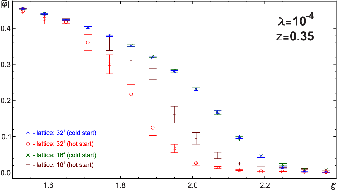
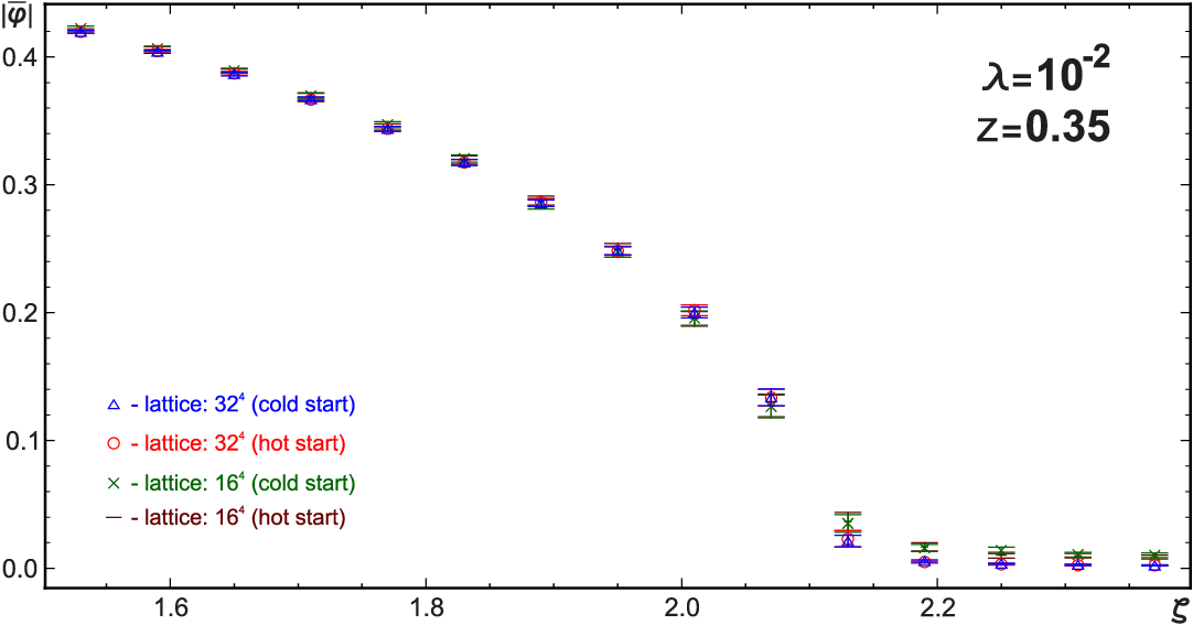
The temperature dependence of for the lattices and at and for is present in Fig. 2. The whole data set for every plot is divided into 15 bins. Different initial conditions are shown as:
- •
hot start – red circles (lattice ) and brown dashes (lattice );
- •
cold start – blue triangles (lattice ) and green crosses (lattice ).
The mean values and 95% confidence intervals are presented by corresponding pointers for each bin. Every bin contains 150 points.
As it is seen from Fig. 2, for the temperature dependence of field condensate is not sensitive to the initial configuration. Both cold and hot starts lead to the same behavior of field condensate for various . This meas a second order phase transition.
For smaller values of the overheated configurations occur in the broken phase for the hot start. That is, different starts demonstrate a hysteresis behavior. This corresponds to a phase transition of the first order.
With further decreasing of , for the behavior of cold and hot starts is completely separated and independent of the temperature. This is plotted in Fig. 2. Such type property probably means that the SSB does not happen even at zero temperature and corresponding value of can be identified with the Linde-Weinberg low bound.
As it is seen in Fig. 2, two different slices and demonstrate the same behavior. The calculations for the slice reproduce the described above results again (see Fig. 3). Thus, the hysteresis occurs at small independently of the model parameters and .

4 Conclusion
As it was discovered in the MC simulations, the temperature phase transition in model is strongly dependent on the coupling value . There is a low bound determining the range where SSB is not realized. Close to this value in the interval the phase transition is first order. For larger values of the second order phase transition happens. These types of the behavior have been determined on the lattices of different sizes independently of the internal model parameters. Our calculation procedure was developed to accelerate the MC procedure in the domain of parameters close to the transition for a wide range of coupling. For usually considered values of it gives the results coinciding with the ones existing in the literature and signalling the second order phase transition. To our knowledge, systematic investigations for smaller values of coupling have not been carried out yet.
Our observations, in particular, may serve as a guide for the applicability of different kind resummations in perturbation theory. In fact, we see that the daisy and super daisy resummations give qualitatively correct results for small values of . For larger values they become non-adequate to the second order nature of the phase transition. In this case other more complicated resummation schemes should be used.
The change of the phase transition type dependently of the coupling value is not a new phenomenon. For instance, in the standard model of elementary particles it is well known that the electroweak phase transition is of first order for small and it converts into a cross-over or even second order one for sufficiently large values of . We have observed that this happens even in the simple model with one coupling.
In the present investigation, we concentrated mainly on the qualitative aspects of converting the phase transition type due to the change of the coupling values. So, we skip an ubiquitous procedure relating the lattice and physical variables, as unessential.
Acknowledgements. The authors are grateful to P.M.Stevenson for useful suggestions. One of us (VD) was supported by DFG under Grant No BO1112/17-1. He also thanks the Institute for Theoretical Physics of Leipzig University for kind hospitality.
References
- [1] J. Zinn-Justin, Int. Ser. Monogr. Phys. 92, 1 - 1008 (1996).
- [2] J. Berges, N. Tetradis and C. Wetterich, Phys. Rept. 363, 223 (2002).
- [3] P. Cea, M. Consoli, L. Cosmai [hep-lat/0407024]; [hep-ph/0311256]; Nucl. Phys. Proc. Suppl. 106, 953 (2002).
- [4] M. Bordag and V. Skalozub, J. Phys. A 34, 461 (2001).
- [5] J. Baacke and S. Michalski, Phys. Rev. D 67, 085006 (2003).
- [6] E. Nakano, V. Skokov and B. Friman, arXiv:1109.6822 [hep-ph].
- [7] E. Seel, Acta Phys. Polon. Supp. 4, 733 (2011).
- [8] N. Petropoulos, hep-ph/0402136.
- [9] A. D. Linde, JETP Lett. 23, 64 (1976).
- [10] S. Weinberg, Phys. Rev. Lett. 36, 294 (1976).
- [11] T. Celik, J. Engels and H. Satz, Phys. Lett. B 125, 411 (1983); F. Karsch, Nucl. Phys. A 418, 467C-476C (1984); B. A. Berg, U. M. Heller, H. Meyer-Ortmanns and A. Velytsky, Phys. Rev. D 69, 034501 (2004).
- [12] V. Demchik and A. Strelchenko, arXiv:0903.3053 [hep-lat].
- [13] V. Demchik, Comput. Phys. Commun. 182 (2011) 692.