Implementation of Decoders for LDPC
Block Codes and LDPC Convolutional
Codes Based on GPUs

A binary $(N,K)$ LDPC code is a linear block code specified by a sparse $M\times N$ parity-check matrix ${\mathbf{H}}$, where $M=N-K$. The code rate of such an LDPC code is $R\geq K/N=1-M/N$. The equality holds when $\mathbf{H}$ is full rank.

The ${\mathbf{H}}$ matrix contains mostly $0^{\prime}s$ and relatively a small number of $1^{\prime}s.$ Such a sparsity structure is the key characteristic that guarantees good performance of LDPC codes. A regular LDPC code is a linear block code with $\mathbf{H}$ containing a constant number $w_{c}$ of $1$’s in each column and a constant number $w_{r}$ of $1$’s in each row. Moreover, $w_{r}$ and $w_{c}$ satisfy the equation $w_{r}=w_{c}\times\frac{N}{M}$. Otherwise the code is defined as an irregular LDPC code.

A bipartite graph called Tanner graph [20] can be used to represent the codes and to visualize the message-passing algorithm. Figure 1 is the underlying Tanner graph of the $\mathbf{H}$ in (1). The $N$ upper nodes are called the message nodes or the variable nodes and the $M$ nodes in the lower part of Fig. 1 are called the check nodes. An edge in the Tanner graph represents the adjacency of the variable node $i$ and the check node $j$. It corresponds to a nonzero $(i,j)$-th entry in the $\mathbf{H}$ matrix.

QC-LDPC codes form a subclass of LDPC codes with the parity-check matrix consisting of circulant permutation matrices [21, 22]. The parity-check matrix of a regular $(J,L)$ QC-LDPC code is represented by

where $J$ denotes the number of block rows, $L$ is the number of block columns, ${\mathbf{P}}$ is the identity matrix of size $p\times p$, and ${\mathbf{P}}^{a_{j,l}}$ ($1\leq j\leq J$; $1\leq l\leq L$) is a circulant matrix formed by shifting the columns of ${\mathbf{P}}$ cyclically to the right $a_{j,l}$ times with $a_{j,l}$’s being non-negative integers less than $p$. The code rate $R$ of ${\mathbf{H}}$ is lower bounded by $R\geq 1-J/L$. If one or more of the sub-matrix(matrices) is/are substituted by the zero matrix rendering non-uniform distributions of the check-node degrees or variable-node degrees, the QC-LDPC code becomes an irregular code.

LDPC codes are most commonly decoded using the belief propagation (BP) algorithm [23, 24]. Referring to the Tanner graph shown in Fig. 1, the variable nodes and the check nodes exchange soft messages iteratively based on the connections and according to a two-phase schedule.

Given a binary (N, K) LDPC code with a parity-check matrix $\mathbf{H}$, we define $\mathcal{C}$ as the set of binary codewords $\mathbf{c}$ that satisfy the equation $\mathbf{c}\mathbf{H}^{\mathrm{T}}=\mathbf{0}$. At the transmitter side, a binary codeword $\mathbf{c}=(c_{0},c_{1},\ldots,c_{N-1})$ is mapped into the sequence $\mathbf{x}=(x_{0},x_{1},\ldots,x_{N-1})$ according to $x_{n}=1-2c_{n}$. We assume that $\mathbf{x}$ is then transmitted over an additive white Gaussian noise (AWGN) channel and the received signal vector is then given by $\mathbf{y}=(y_{0},y_{1},\ldots,y_{N-1})=\mathbf{x}+\mathbf{g}$, where $\mathbf{g}=(g_{0},g_{1},\ldots,g_{N-1})$ consists of independent Gaussian random variables with zero mean and variance $\sigma^{2}=N_{0}/2$.

Let $\mu_{n}$ be the initial log-likelihood ratio (LLR) that the variable node $n$ is a “$0$” to that it is a “$1$”, i.e.,

Initially, $\mu_{n}$ is calculated by $\mu_{n}=(4/N_{0})\cdot y_{n}=\frac{2y_{n}}{\sigma^{2}}$ [25]. Define $\mathcal{N}(m)$ as the set of variable nodes that participate in check node $m$ and $\mathcal{M}(n)$ as the set of check nodes connected to variable node $n$. At iteration $i$, let $\beta_{mn}^{(i)}$ be the LLR messages passed from variable node $n$ to check node $m$; $\alpha_{mn}^{(i)}$ be the LLR messages passed from check node $m$ to variable node $n$; and $\beta_{n}^{(i)}$ be the a posteriori LLR of variable node $n$. Then the standard BP algorithm can be described in Algorithm 1 [2, 26].

Note that the decoding algorithm consists of 4 main procedures: initialization, horizontal step, vertical step and making hard decisions. For each of these procedures, multiple threads can be used in executing the computations in parallel and all the threads will follow the same instructions with no divergence occurring, except when making hard decisions.

A (time-varying) semi-infinite LDPC convolutional code can be represented by its parity check matrix in (3).

where $m_{s}$ is referred to as the syndrome former memory of the parity-check matrix. Besides, the sub-matrices ${\mathbf{H}}_{i}(t),i=0,1,...,m_{s}$, are binary $(c-b)\times c$ matrices given by

If ${\mathbf{H}}_{i}(t)$ are full rank for all time instant $t$, the matrix ${\mathbf{H}}$ in (3) defines a rate $R=b/c$ convolutional code ignoring the irregularity at the beginning.

A code sequence ${\mathbf{v}}_{[0,\infty]}$ = $[{\mathbf{v}}_{0},{\mathbf{v}}_{1},...,{\mathbf{v}}_{\infty}]$ is “valid” if it satisfies the equation

where ${\mathbf{v}}_{i}$ = $(v_{i}^{(1)},v_{i}^{(2)},...,v_{i}^{(c)})$ and ${\mathbf{H}}_{[0,\infty]}^{T}$ is the syndrome-former (transposed parity-check) matrix of ${\mathbf{H}}_{[0,\infty]}$.

There are several methods to construct LDPC convolutional codes from LDPC block codes. One method is to derive time-varying LDPCCC by unwrapping randomly constructed LDPC block codes [17] and another is by unwrapping the QC-LDPC codes [27, 28]. We now consider a construction method by unwrapping a class of QC-LDPC block code.

Suppose we have created a $(J,L)$ QC-LDPC block code ${\mathbf{H}}_{QC}$ with $J$ block-rows and $L$ block-columns. The size of its circulant matrices is $p\times p$. We can derive the parity-check matrix for a LDPC convolutional code using the following steps.

1. 1.

   Partition the $pJ\times pL$ parity-check matrix ${\mathbf{H}}_{QC}$ to form a $\Lambda\times\Lambda$ matrix, where $\Lambda$ is the greatest common divisor of $J$ and $L$, i.e.,

   $${\mathbf{H}}_{QC}=\begin{bmatrix}{\mathbf{H}}_{1,1}&{\mathbf{H}}_{1,2}&\cdots&{\mathbf{H}}_{1,\Lambda}\\ {\mathbf{H}}_{2,1}&{\mathbf{H}}_{2,2}&\cdots&{\mathbf{H}}_{2,\Lambda}\\ \vdots&\vdots&\cdots&\vdots\\ {\mathbf{H}}_{\Lambda,1}&{\mathbf{H}}_{\Lambda,2}&\cdots&{\mathbf{H}}_{\Lambda,\Lambda}\end{bmatrix}_{\Lambda\times\Lambda},$$

   where ${\mathbf{H}}_{i,j}$ is a $(pJ/\Lambda)\times(pL/\Lambda)$ matrix, for $i,j=1,2,...,\Lambda$.

2. 2.

   Divide ${\mathbf{H}}_{QC}$ along the diagonal into two portions: the strictly upper-triangular portion ${\mathbf{H}}_{QC}^{(U)}$ and the lower-triangular portion ${\mathbf{H}}_{QC}^{(L)}$ as follows:

   $${\mathbf{H}}_{QC}^{(U)}=\begin{bmatrix}\mathbf{0}&{\mathbf{H}}_{1,2}&{\mathbf{H}}_{1,3}&\cdots&{\mathbf{H}}_{1,\Lambda}\\ &\mathbf{0}&{\mathbf{H}}_{2,3}&\cdots&{\mathbf{H}}_{2,\Lambda}\\ &&\ddots&\cdots\vdots\\ &&&\mathbf{0}&{\mathbf{H}}_{\Lambda-1,\Lambda}\\ &&&&\mathbf{0}\end{bmatrix}_{\Lambda\times\Lambda},$$

   and

   $${\mathbf{H}}_{QC}^{(L)}=\begin{bmatrix}{\mathbf{H}}_{1,1}&&&\\ {\mathbf{H}}_{2,1}&{\mathbf{H}}_{2,2}&&\\ \vdots&\vdots&\ddots&\\ {\mathbf{H}}_{\Lambda,1}&{\mathbf{H}}_{\Lambda,2}&\cdots&{\mathbf{H}}_{\Lambda,\Lambda}\end{bmatrix}_{\Lambda\times\Lambda}.$$

3. 3.

   Unwrap the parity-check matrix of the block code to obtain the parity-check matrix of LPDCCC. First paste the strictly upper-triangular portion below the lower-triangular portion. Then repeat the resulting diagonally-shaped matrix infinitely, i.e.,

   $${\mathbf{H}}_{conv}=\begin{bmatrix}{\mathbf{H}}_{QC}^{L}&&&\\ {\mathbf{H}}_{QC}^{U}&{\mathbf{H}}_{QC}^{L}&&\\ &{\mathbf{H}}_{QC}^{U}&{\mathbf{H}}_{QC}^{L}&\\ &&\ddots&\ddots\\ \end{bmatrix}.$$

The resulting time-varying LDPCCC has a period of $T=\Lambda$ and the memory $m_{s}$ equals $\Lambda-1$. The girth of the derived LPDCCC is at least as large as the girth of the QC-LDPC code [29]. A convenient feature of this time-varying unwrapping is that a family of LDPC convolutional codes can be derived by choosing different circulant size $p$ of the QC-LDPC block code.

In ${\mathbf{H}}_{[0,\infty]}$, two different variable nodes connected to the same check node cannot be distant from each other more than $m_{s}$ time units. This allows a decoding window that operates on a fixed number of nodes at one time. Since any two variable nodes that are at least $m_{s}+1$ units apart can be decoded independently, parallel implementation is feasible. The LDPCCC can therefore be decoded with pipelined BP decoding algorithm [17]. Specifically, for a maximum iteration number of $I$, $I$ independent processors will be employed working on different variable nodes corresponding to different time. In each processor, the variable nodes and the check nodes exchange soft messages iteratively based on the connections and according to a two-phase schedule.

Fig. 3 shows a decoder on the Tanner graph. It is based on the LDPCCC structure shown in Example 1. The code has a rate of $R=5/6$ and a syndrome former memory of $m_{s}=3$. We refer the $c$ incoming variable nodes (bits) as a frame. Note that every $c$ bits form a frame and every $m_{s}+1$ frames are involved in the same constraints. The $I$ processors can operate concurrently. At every iteration, every processor first updates the $(c-b)$ neighboring check nodes of the $c$ variable nodes that just come into this processor. Then every processor will update the $c$ variables which are leaving this processor.

The computations of the check-node updating and variable-node updating are based on the standard BP algorithm Suppose ${\mathbf{v}}_{[0,\infty]}$ = $[{\mathbf{v}}_{0},{\mathbf{v}}_{1},\ldots,{\mathbf{v}}_{\infty}]$, where ${\mathbf{v}}_{t}=(v_{t}^{(1)},v_{t}^{(2)},\ldots,v_{t}^{(c)})$ is the $t$th transmitted codeword. Then the codeword ${\mathbf{v}}_{[0,\infty]}$ is mapped into the sequence ${\mathbf{x}}_{[0,\infty]}=[{\mathbf{x}}_{0},{\mathbf{x}}_{1},\ldots,{\mathbf{x}}_{\infty}]$ according to ${\mathbf{x}}_{t}=(x_{t}^{(1)},x_{t}^{(2)},\ldots,x_{t}^{(c)})$ and $x_{t}^{(j)}=1-2v_{t}^{(j)}$ ($j=1,2,\ldots,c$). Assuming an AWGN channel, the received signal ${\mathbf{y}}_{[0,\infty]}=[{\mathbf{y}}_{0},{\mathbf{y}}_{1},\ldots,{\mathbf{y}}_{\infty}]$ is further given by ${\mathbf{y}}_{t}=(y_{t}^{(1)},y_{t}^{(2)},\ldots,y_{t}^{(c)})$ where $y_{t}^{(j)}=x_{t}^{(j)}+g_{t}^{(j)}$ and $g_{t}^{(j)}$ is an AWGN with zero mean and variance $\sigma^{2}=N_{0}/2$.

Using the same notation as in Sect. II-B, the pipelined BP decoding algorithm applying to LDPCCC is illustrated in Algorithm 2. Same as the LDPC decoding algorithm, the LDPCCC decoding algorithm consists of 4 main procedures: initialization, horizontal step, vertical step and making hard decisions. Moreover, for each of these procedures, multiple threads can be used in executing the computations in parallel and all the threads will follow the same instructions with no divergence occurring, except when making hard decisions.

We implement our decoders using the standard BP decoding algorithm. According to the CUDA programming model, the granularity of a thread execution and a coalesced memory access is a warp. Full efficiency is realized when all threads in a warp take the same execution path and the coalesced memory access requirement is satisfied. Thus, we propose to decode $\Gamma$ codewords simultaneously, where $\Gamma$ is an integer multiple of a warp (i.e., multiple of 32). For each decoding cycle, $\Gamma$ codewords will be input, decoded, and ouput together and in parallel.

Recall that an LDPC code can be represented by its parity-check matrix or a Tanner graph. A non-zero element in the parity-check matrix corresponds to an edge in the Tanner graph.

In the LDPC decoder, messages are bound to the edges in the Tanner graph (or the $1$’s in the parity-check matrix ${\mathbf{H}}$). So we store the messages according to the positions of $1$’s. Besides, the channel messages corresponding to the variable nodes are required. To reuse the notation, we denote the data structure storing the messages between the variable nodes and the check nodes as ${\mathbf{H}}$ while the the data structure storing the channel messages as ${\mathbf{V}}$. The difficulty of the CUDA memory arrangement lies on the fact that for practical LDPC codes with good performance, the positions of the $1$’s are scattered in the parity-check matrix.

First, in the BP decoding procedure, although there are two kinds of messages, namely, the variable-to-check messages and the check-to-variable messages, at every step of the iteration, only one kind of message is needed to be stored, i.e., after the check-node updating step, only the check-to-variable messages $\alpha$’s are stored in the ${\mathbf{H}}$ and after the variable-node updating step, only the variable-to-check messages $\beta$’s are stored in the ${\mathbf{H}}$. Second, in our new decoder architecture, $\Gamma$ ($\Gamma$ is a multiple of a warp) codewords are decoded together and hence the messages of $\Gamma$ codewords are also processed together. We number the distinct codewords as $0,1,...,\Gamma-1$ and we use the same notations for the messages as before, i.e., $\beta_{mn}(\gamma)$ is the message from variable node $n$ to check node $m$ corresponding to the $\gamma$-th codeword and $\alpha_{mn}(\gamma)$ is the message from check node $m$ to variable node $n$ corresponding to the $\gamma$-th codeword. Since all the $\Gamma$ codewords messages share the same Tanner graph, messages of the $\Gamma$ distinct codewords corresponding to the same edge can be grouped into one package and stored linearly. Let ${\mathfrak{p}}_{mn}$ denote the package corresponding to the edge connecting variable node $n$ and check node $m$. Then in package ${\mathfrak{p}}_{mn}$, $\beta_{mn}(0),\beta_{mn}(1),...,\beta_{mn}(\Gamma-1)$ or $\alpha_{mn}(0),\alpha_{mn}(1),...,\alpha_{mn}(\Gamma-1)$ are stored contiguously. This is shown in Figure 5. Different packages ${\mathfrak{p}}_{mn}$’s are aligned linearly according to their corresponding positions in the parity-check matrix — row-by-row, and left to right for each row. That implies the messages associated to one check node are stored contiguously.

The advantage of this arrangement is obvious. Since $\Gamma$ is a multiple of 32, the memory segment for every package is naturally aligned when the data type belongs to one of the required data types (i.e., with word size of 1-, 2-, 4-, or 8-byte). In addition, the structure of the parity-check matrix ${\mathbf{H}}$ is shared by the $\Gamma$ codewords. As these $\Gamma$ data elements are processed together, they can be accessed by $\Gamma$ contiguous threads and hence the global memory is always accessed in a coalesced way. We also ensure that the threads within a warp always follow the same execution path with no divergence occurring (except when making hard decisions on the received bits). Then both the memory access and the thread execution are optimal and efficient.

We also need to store the details of the parity-check matrix. Two lookup tables denoted by $LUT_{c}$ and $LUT_{v}$ will be kept. $LUT_{c}$ is used in the check-node updating process and $LUT_{v}$ is used in the variable-node updating process. The two tables store the indices of the data accessed in the two updating processes and both are two-dimensional. The first dimension is to distinguish different check nodes, i.e., $LUT_{c}[m]$ is associated with the $m$-th check node or the $m$-th row. Each $LUT_{c}[m]$ records the indices of the messages related to the $m$-th check node. The two lookup tables are shared by all $\Gamma$ codewords.

A separate thread is assigned to process each check node or each variable node in the updating kernel. Hence, $\Gamma$ threads can be assigned to process the data of $\Gamma$ codewords simultaneously. So, a two dimensional thread hierarchy is launched. The first dimension is for identifying the different codewords while the second dimension is for processing different check nodes or variable nodes. The thread layout is illustrated in Fig. 6. For each thread block, we allocate $\Gamma$ threads in the threadIdx.x dimension²² 2 In CUDA, threads are linear in the threadIdx.x dimension., and $BL_{y}$ threads in the threadIdx.y dimension. Each thread-block contains $BL_{y}\times\Gamma$ threads, which should be within the thread-block size limit (1024 for the current device). The total number of thread-blocks is determined by the number of check nodes $M$ or the number of variable nodes $N$. We denote $BL_{y}$ in the check-node updating kernel as $BL_{y,cnu}$ and the one in the variable-node updating kernel as $BL_{y,vnu}$. Then the numbers of thread blocks are given by $\lceil M/BL_{y,cnu}\rceil$ and $\lceil N/BL_{y,vnu}\rceil$, respectively. In Fig. 6, the threads marked by the vertical rectangular are processing the same codeword.

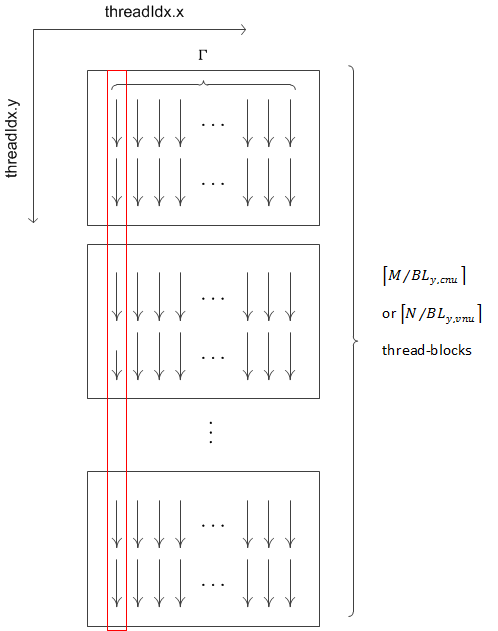
In the check-node updating kernel and the variable-node updating kernel, the forward-and-backward calculation is adopted as in [32]. The shared memory is used to cache the involved data so as to avoid re-accessing the global memory. Due to the limited size of the shared memory, the size of the thread-block should not be too large. Consider a $(J,L)$ QC-LDPC code. For each check node, there are $2L$ data elements to be stored. Denote the shared memory size by $Z_{{\rm shared}}$ and the size of each data by $Z_{{\rm data}}$. Consequently in the check-node updating kernel, the thread-block size, denoted by $\Omega_{{\rm cnu}}$, is limited by

In addition, $\Omega_{{\rm cnu}}=BL_{y,cnu}\times\Gamma$ and $\Omega_{\rm vnu}=BL_{y,vnu}\times\Gamma$.

With such a thread layout, the threads access the memory in a straightforward pattern. For example, for the check-node updating kernel, a two-dimensional thread hierarchy with a total size of $\lceil\frac{M}{BL_{y,cnu}}\rceil\times BL_{y,cnu}\times\Gamma$ is launched. During the memory access, every $\Gamma$ threads are one-to-one mapped to $\Gamma$ data in a message package. Hence, coalesced memory access is guaranteed.

The decoding algorithm and the pipelined LDPCCC decoder architecture have been introduced in Section II-E. The LDPCCCs studied in our work are derived from QC-LDPC codes as described in Section II-D. So our LDPCCC decoder is confined to the LDPCCCs with the parity-check matrix ${\mathbf{H}}_{[0,\infty]}$ of this kind of structure.

We implement both the serial CPU-based LDPC decoder and LDPCCC decoder using the C language. As CPUs with multiple cores are very common nowadays, we further implement a multi-thread CPU-based LDPCCC decoder using OpenMP. OpenMP [33] is a portable, scalable programming interface for shared-memory parallel computers. It can be used to explicitly direct multi-threaded, shared memory parallelism. A straightforward application of the OpenMP is to parallize the intensive loop-based code with the #pragma omp parallel for directive. Then the executing threads will be automatically allocated to different cores on a multi-core CPU.

The horizontal step and the vertical step in Algorithm 2 involve intensive computing. On a single-core CPU, the updating of the different nodes are processed with a serial for loop. Since the updating of different nodes can be performed independent of one another, it is ideal to parallelize the for loop with the #pragma omp parallel for directive in the OpenMP execution on a multicore CPU. Hence, in our implementation, we issue multiple threads to both the updating of the check nodes (9) and the updating of the variable nodes (10) in the multi-thread CPU-based LDPCCC decoder.

The CPU being used is an Intel Xeon containing $4$ cores. Moreover, it can handle up to $8$ threads at a time. The serial CPU-based decoders are developed using C and the multi-threaded CPU-based LDPCCC decoder is developed using OpenMP. Note that for the serial CPU-based decoders, only one of the $4$ cores in the CPU will be utilized. The GPU used in this paper is a GTX460 containing $336$ cores and the GPU-based decoders are developed using CUDA C. Furthermore, in our simulations, $32$ codewords are decoded simultaneously in the GPU decoders, i.e., $\Gamma=32$. Details of the CPU and GPU used in our simulations are presented in Table I.

Table II shows the characteristics of the QC-LDPC codes under test. For Code A to code D, $J=4$ and $L=24$ thus giving the same code rate of $(24-4)/24=5/6$. These codes are further used to derived regular LDPCCCs. In order to avoid confusion, we denote the derived LDPCCCs as Code A’ to Code D’. It can be readily shown that the $(3,4,24)$-LDPCCCs A’ to D’ have the same code rate of $5/6$.

References

- [1] R. G. Gallager, Low-Density Parity-Check Codes. The MIT Press, Sep. 1963.
- [2] D. MacKay, “Good error-correcting codes based on very sparse matrices,” Information Theory, IEEE Transactions on, vol. 45, no. 2, pp. 399–431, 1999.
- [3] I. Djordjevic, M. Cvijetic, L. Xu, and T. Wang, “Using LDPC-Coded modulation and coherent detection for ultra highspeed optical transmission,” Lightwave Technology, Journal of, vol. 25, no. 11, pp. 3619–3625, 2007.
- [4] Y. Miyata, K. Sugihara, W. Matsumoto, K. Onohara, T. Sugihara, K. Kubo, H. Yoshida, and T. Mizuochi, “A triple-concatenated FEC using soft-decision decoding for 100 Gb/s optical transmission,” in Optical Fiber Communication (OFC), collocated National Fiber Optic Engineers Conference, 2010 Conference on (OFC/NFOEC), 2010, pp. 1–3.
- [5] Y. Chen and D. Hocevar, “A FPGA and ASIC implementation of rate 1/2, 8088-b irregular low density parity check decoder,” in Global Telecommunications Conference, 2003. GLOBECOM ’03. IEEE, vol. 1, 2003, pp. 113–117 Vol.1.
- [6] I. B. Djordjevic, M. Arabaci, and L. L. Minkov, “Next generation FEC for High-Capacity communication in optical transport networks,” Journal of Lightwave Technology, vol. 27, no. 16, pp. 3518–3530, 2009.
- [7] B. Levine, R. R. Taylor, and H. Schmit, “Implementation of near Shannon limit error-correcting codes using reconfigurable hardware,” 2000.
- [8] A. Pusane, A. Feltstrom, A. Sridharan, M. Lentmaier, K. Zigangirov, and D. Costello, “Implementation aspects of LDPC convolutional codes,” Communications, IEEE Transactions on, vol. 56, no. 7, pp. 1060–1069, 2008.
- [9] S. Bates, Z. Chen, L. Gunthorpe, A. Pusane, K. Zigangirov, and D. Costello, “A low-cost serial decoder architecture for low-density parity-check convolutional codes,” Circuits and Systems I: Regular Papers, IEEE Transactions on, vol. 55, no. 7, pp. 1967 –1976, Aug. 2008.
- [10] Z. Chen, S. Bates, and W. Krzymien, “High throughput parallel decoder design for LDPC convolutional codes,” in Circuits and Systems for Communications, 2008. ICCSC 2008. 4th IEEE International Conference on, May 2008, pp. 35 –39.
- [11] R. Swamy, S. Bates, and T. Brandon, “Architectures for asic implementations of low-density parity-check convolutional encoders and decoders,” in Proc. IEEE Int. Symp. Circuits and Systems ISCAS 2005, 2005, pp. 4513–4516.
- [12] G. Falcao, V. Silva, and L. Sousa, “How GPUs can outperform ASICs for fast LDPC decoding,” in Proceedings of the 23rd international conference on Supercomputing. Yorktown Heights, NY, USA: ACM, 2009, pp. 390–399.
- [13] H. Ji, J. Cho, and W. Sung, “Massively parallel implementation of cyclic LDPC codes on a general purpose graphics processing unit,” in Signal Processing Systems, 2009. SiPS 2009. IEEE Workshop on. IEEE, 2009, pp. 285–290.
- [14] ——, “Memory access optimized implementation of cyclic and quasi-cyclic LDPC codes on a GPGPU,” Journal of Signal Processing Systems, pp. 1–11, 2010.
- [15] G. Falcao, L. Sousa, and V. Silva, “Massive parallel LDPC decoding on GPU,” in Proceedings of the 13th ACM SIGPLAN Symposium on Principles and practice of parallel programming. Salt Lake City, UT, USA: ACM, 2008, pp. 83–90.
- [16] ——, “Massively LDPC decoding on multicore architectures,” IEEE Transactions on Parallel and Distributed Systems, vol. 22, no. 2, pp. 309–322, Feb. 2011.
- [17] A. J. Felstrom and K. Zigangirov, “Time-varying periodic convolutional codes with low-density parity-check matrix,” Information Theory, IEEE Transactions on, vol. 45, no. 6, pp. 2181–2191, 1999.
- [18] M. Tavares, E. Matus, S. Kunze, and G. Fettweis, “A dual-core programmable decoder for LDPC convolutional codes,” in Circuits and Systems, 2008. ISCAS 2008. IEEE International Symposium on, May 2008, pp. 532 –535.
- [19] E. Matus, M. Tavares, M. Bimberg, and G. Fettweis, “Towards a GBit/s programmable decoder for LDPC convolutional codes,” in Circuits and Systems, 2007. ISCAS 2007. IEEE International Symposium on, May 2007, pp. 1657 –1660.
- [20] R. Tanner, “A recursive approach to low complexity codes,” Information Theory, IEEE Transactions on, vol. 27, no. 5, pp. 533–547, 1981.
- [21] M. Fossorier, “Quasicyclic low-density parity-check codes from circulant permutation matrices,” Information Theory, IEEE Transactions on, vol. 50, no. 8, pp. 1788–1793, 2004.
- [22] W. Tam, F. Lau, and C. Tse, “A class of QC-LDPC codes with low encoding complexity and good error performance,” Communications Letters, IEEE, vol. 14, no. 2, pp. 169–171, 2010.
- [23] T. Richardson, M. Shokrollahi, and R. Urbanke, “Design of capacity-approaching irregular low-density parity-check codes,” Information Theory, IEEE Transactions on, vol. 47, no. 2, pp. 619–637, 2001.
- [24] T. Richardson and R. Urbanke, “Efficient encoding of low-density parity-check codes,” Information Theory, IEEE Transactions on, vol. 47, no. 2, pp. 638–656, 2001.
- [25] X. Hu, E. Eleftheriou, D. Arnold, and A. Dholakia, “Efficient implementations of the sum-product algorithm for decoding LDPC codes,” in Global Telecommunications Conference, 2001. GLOBECOM ’01. IEEE, vol. 2, 2001, pp. 1036–1036E vol.2.
- [26] J. Chen, A. Dholakia, E. Eleftheriou, M. Fossorier, and X. Hu, “Reduced-Complexity decoding of LDPC codes,” Communications, IEEE Transactions on, vol. 53, no. 8, pp. 1288–1299, 2005.
- [27] R. Tanner, D. Sridhara, A. Sridharan, T. Fuja, and D. Costello, “LDPC block and convolutional codes based on circulant matrices,” Information Theory, IEEE Transactions on, vol. 50, no. 12, pp. 2966–2984, 2004.
- [28] A. E. Pusane, R. Smarandache, P. O. Vontobel, and D. J. Costello, “On deriving good LDPC convolutional codes from QC-LDPC block codes,” in Proc. IEEE Int. Symp. Information Theory ISIT 2007, 2007, pp. 1221–1225.
- [29] M. Lentmaier, D. G. M. Mitchell, G. P. Fettweis, and D. J. Costello, “Asymptotically regular LDPC codes with linear distance growth and thresholds close to capacity,” in Proc. Information Theory and Applications Workshop (ITA), 2010, pp. 1–8.
- [30] C. Nvidia, “Compute Unified Device Architecture Programming Guide Version 4.0,” NVIDIA Corporation, Tech. Rep., 2011.
- [31] W. Nvidia, N. Generation, and C. Compute, “Whitepaper nvidia’s next generation cuda compute architecture,” ReVision, pp. 1–22, 2009.
- [32] F. Kschischang, B. Frey, and H. Loeliger, “Factor graphs and the sum-product algorithm,” Information Theory, IEEE Transactions on, vol. 47, no. 2, pp. 498–519, 2001.
- [33] R. Chandra, Parallel programming in OpenMP. Morgan Kaufmann, 2001.