Entanglement-Assisted Quantum Error-Correcting Codes with Imperfect Ebits
Abstract
The scheme of entanglement-assisted quantum error-correcting (EAQEC) codes assumes that the ebits of the receiver are error-free. In practical situations, errors on these ebits are unavoidable, which diminishes the error-correcting ability of these codes. We consider two different versions of this problem. We first show that any (nondegenerate) standard stabilizer code can be transformed into an EAQEC code that can correct errors on the qubits of both sender and receiver. These EAQEC codes are equivalent to standard stabilizer codes, and hence the decoding techniques of standard stabilizer codes can be applied. Several EAQEC codes of this type are found to be optimal. In a second scheme, the receiver uses a standard stabilizer code to protect the ebits, which we call a “combination code.” The performances of different quantum codes are compared in terms of the channel fidelity over the depolarizing channel. We give a formula for the channel fidelity over the depolarizing channel (or any Pauli error channel), and show that it can be efficiently approximated by a Monte Carlo calculation. Finally, we discuss the tradeoff between performing extra entanglement distillation and applying an EAQEC code with imperfect ebits.
I Introduction
The theory of quantum error correction is important for both quantum computation and quantum communication [1, 2, 3, 4, 5, 6]. Quantum stabilizer codes are the most extensively studied quantum codes [7, 8], and have the advantage that their properties can be analyzed using group algebra. Quantum stabilizer codes are closely related to classical linear codes, and can be obtained by the CRSS and CSS code constructions from weakly self-dual classicalcodes [9, 10, 7, 11, 8, 12]. When entanglement between sender and receiver is available, a new error correction scheme becomes possible: entanglement-assisted quantum error-correction. This coding scheme (EAQEC codes) has the advantage that it allows any classical linear code, not necessarily weakly self-dual, to be transformed into a quantum code [13]. In addition, EAQEC codes can increase both the transmission rate and error-correcting ability [14, 15]. Also, some problems or limitations in quantum LDPC codes and turbo codes can be solved using EAQEC codes [15, 16].
In EAQEC codes [13], it is assumed that the sender (Alice) and the receiver (Bob) share some pairs of qubits in maximally-entangled states (ebits) before communication, and the quits on Bob’s side are subject to no error. The quantum codes are designed to cope with the noisy channel that Alice uses to communicate with Bob. The properties of EAQEC codes in this case are studied in [13, 14, 17]. However, noise (such as storage errors) can occur on Bob’s ebits in practical situations, which is believed to degrade the performance of the quantum codes.
Assume the errors occurring on Bob’s qubits are described by a noise process . Wilde and Hsieh addressed this question with a channel-state coding protocol in quantum Shannon theory and determined the channel capacity when entanglement is not perfect [18]. They also performed simulations of entanglement-assisted quantum turbo codes with the depolarizing channel when Bob’s ebits also suffer errors [15]. Wilde and Fattal simulated the performance of an entanglement-assisted Steane code for fault tolerance [19].
In this article, we discuss two coding schemes to handle the problem when the ebits of Bob are not perfect. Shaw et al. described a six-qubit EAQEC code with one ebit that is equivalent to Steane’s seven-qubit code, and can correct a single error on either Alice’s or Bob’s qubits [20]. The entanglement-assisted Steane code, constructed by Wilde and Fattal, is also equivalent to Steane’s seven-qubit code [19]. Similarly, Bowen’s entanglement-assisted code [21] is equivalent to the five-qubit code [5, 22] and can correct an error on one of Bob’s qubits. These three examples motivate the following idea: there are EAQEC codes that are equivalent to standard stabilizer codes, and hence can correct errors on both Alice’s and Bob’s sides. We show how to obtain an EAQEC code from a (nondegenerate) stabilizer code. Several EAQEC codes from this scheme are found to be optimal. We say a quantum code is optimal if the minimum distance of this code achieves an upper bound for fixed numbers of information qubits and physical qubits. These EAQEC codes will have better performance than their equivalent stabilizer codes when the storage error rate is less than the channel error rate.
In the second scheme, Alice uses an EAQEC code to encode her information qubits and Bob uses a standard stabilizer code to protect his halves of the ebits. The combination of an EAQEC code and a stabilizer code is called a combination code, and it can be treated either as a single stabilizer code, or by using two sequential decoders. EAQEC codes that are not equivalent to standard stabilizer codes generally have higher error-correcting ability on Alice’s qubits and are suitable for this scheme.
Minimum distance of a stabilizer code is used as a measure of how good a code is without considering the details of the noisy channel model. However, minimum distance might not always be the best measure, for a quantum code may be able to correct many error operators of weight higher than that indicated by the minimum distance. In particular, there is no general definition of minimum distance for the variant coding schemes in this article. A perhaps more suitable merit function is the channel fidelity [23, 24], which compares the similarity of the modified quantum state with the original quantum state. However, the calculation of the channel fidelity depends on the channel and has an exponentially increasing complexity. We derive a formula for the channel fidelity of a quantum stabilizer code over the depolarizing channel, which facilitates its computation. The channel fidelity also can be well approximated by a lower bound when the depolarizing rate is small. Furthermore, Monte Carlo methods can often efficiently approximate the channel fidelity [25].
Another natural question arises in EAQEC codes. The perfect entanglement shared between sender and receiver will in practice be generated from a process of entanglement distillation [26, 5] or a breeding protocol [27]. It is known that entanglement distillation with one-way classical communication is equivalent to a quantum error-correcting code [5]. Since we can also communicate using an EAQEC code that is robust to imperfect ebits, we discuss whether it is always necessary to do entanglement distillation before communication, and how much.
This paper is structured as follows. Basics of stabilizer codes and EAQEC codes are reviewed in the next section. Basic criteria for an EAQEC code to be capable of correcting errors on Bob’s qubits are analyzed in Section III. We discuss the first coding scheme with imperfect ebits in Section IV, and the second scheme in Section V. The formula for the channel fidelity over the depolarizing channel is derived in Section VI, and the channel fidelities for quantum stabilizer codes and EAQEC codes are given in Subsection VI.1 and VI.2, respectively. We discuss Monte Carlo simulations for the channel fidelity in Subsection VI.3. In Section VII, we compare the performances of different coding schemes in terms of the channel fidelity. Entanglement distillation is discussed in Section VIII. The conclusions follow in Section IX.
II Basics
Let be the state space of a single qubit. Suppose Alice sends a -qubit state to Bob by using an quantum stabilizer code that encodes the qubit information state in a -dimensional subspace of the -qubit state space , fixed by a stabilizer group with some minimum distance . The stabilizer group is an Abelian subgroup of the -fold Pauli group , with generators , and does not contain the negative identity operator . Suppose is an -fold unitary Clifford encoder, which leaves the -fold Pauli group invariant under conjugation. The encoded state is . For convenience, let the stabilizer generators be for , where the subscript of the Pauli operator means that the operator is on the -th qubit. The error-correction condition for stabilizer codes says that is a set of correctable error operators in if [8, 12], where is the normalizer group of in . (Since the the overall phase of a quantum state is not important, we consider errors of the form , where for .) This implies the definition of the minimum distance of a stabilizer code to be the minimum weight of any element in , where the weight of is the number of components of that are not equal to the identity.
After Bob receives the noisy quantum state, he does the following three steps to recover the information state : syndrome measurement, correction, and decoding. He first applies a series of projective measurements with projectors
on the output state of the noisy channel. Here, is a binary -tuple that represents the error syndrome. The error syndrome of an error operator has if commutes with and otherwise. We sometimes represent as a number with binary form . Note that the ’s are orthogonal to each other, and is the projector on the code space, that is,
for any -qubit state . Given a stabilizer group , there are distinct error syndromes. For each nonzero error syndrome , we choose a Pauli operators (not in ), whose error syndrome is ; for the error syndrome , we choose . The error operators are called syndrome representatives. If the measurement result is , the correction operator is applied, followed by the decoding unitary operator . Finally, Bob throws away the ancilla qubits, which is the same as applying a partial trace over the ancilla qubits. We define a set containing the syndrome representatives . Then and is a set of correctable error operators. Note that the choice of determines the decoding process. ( determines the encoding process.) In fact, we have many more correctable error operators than . For , the operation of and on the encoded state are the same () and can be corrected by the the same correction operator . The error operator is called a degenerate error of . The set is a correctable set of error operators that satisfies the error correction condition.
Lemma 1.
For a given , the error operators in are correctable and are the only correctable error operators.
Therefore, we have a total of correctable -fold Pauli operators. Note that a code can have different and inequivalent sets .
In this article, error processes are modeled by the depolarizing channel independently operating on qubits, where
with depolarizing rate for and the density operator of a single qubit. Since the operation elements of the depolarizing channel are and , the operation elements of are , where is a Pauli operator in the -fold Pauli group and is the probability that error happens. If is of weight , then is
| (1) |
Now assume maximally-entangled states are shared between Alice and Bob. Suppose Alice uses an -fold Clifford encoder to encode a -qubit state in physical qubits (including the halves of the ebits on Alice’s side) and then sends it to Bob. This is called an EAQEC code for some minimum distance . The encoded state is
where the superscript or indicates that the operator acts on the qubits of Alice or Bob, respectively. Let and for . The encoded state is stabilized by for , for , and for . These ’s and ’s are called simplified stabilizer generators. (We will omit the superscripts as there is no ambiguity.) Note that and anti-commute with each other and they commute with all other generators and for . Thus and are symplectic partners for . An EAQEC code is defined by the simplified stabilizer group of the encoded state:
The symplectic subgroup of is , , , , and the isotropic subgroup of is , . , so that is generated by the generators of and . The minimum distance of the EAQEC code is the minimum weight of any element in [13]. The decoding process of an EAQEC code is similar to that of a standard stabilizer code.
III Determining the Syndrome Representatives for EAQEC Codes
For a channel with low error rate, we would like to choose the set of syndrome representatives to contain lower-weight error operators, since these errors are more likely to occur. A simple algorithm to define a set is as follows:
- (a)
Let and
- (b)
Find an error operator with the lowest weight, and compute its syndrome .
- (c)
If there is no , set and .
- (d)
If there is an , set .
- (e)
If , go to (b). Else, output .
This algorithm finds a set of minimum weight, that is, it minimizes the quantity
In the usual paradigm of EAQEC codes, it is assumed that Bob’s qubits suffer no error. However, this assumption might not be true in practice. Suppose that Alice uses a noisy channel to communicate with Bob and Bob’s ebits suffer from a storage error channel . Assume both and are depolarizing channels. Let and be the depolarizing rate of and , respectively. Define
| (2) |
for , and
| (3) |
for . An error operator of occurs with probability , where and .
To correct some errors on Bob’s qubits, we have to design a quantum code such that these errors are either syndrome representatives, or degenerate errors of other correctable errors. It is more complicated to determine the syndrome representatives in the case of EAQEC codes, since the error probabilities are different on Alice’s and Bob’s qubits. For an EAQEC code to correct some errors on Bob’s qubits, we must sacrifice some of its ability to correct channel errors. For example, consider Bowen’s code with the following stabilizer generators:
Alice’s qubits and Bob’s qubits are on the left and the right of the vertical line, respectively. The error operators and have the same error syndrome. is an error operator on Bob’s side with probability
If Bob’s qubits are error free, the code can correct the weight-2 error on Alice’s side, which occurs with probability
We can instead choose to correct if . This is a tradeoff between correcting channel errors or storage errors. We plot as a function of and in Fig. 1. It can be seen that is a more likely error than when is small or is large.

To sum up, the set of syndrome representatives should be chosen to minimize
We will show that this criterion leads to high channel fidelity in Section VI. We propose two coding schemes in the next two sections.
IV EAQEC Codes that are Equivalent to Standard Stabilizer Codes
The stabilizer generators of the five qubit code [12] are:
After some row operations, these are equivalent to the stabilizer generators of Bowen’s EAQEC code in (III). Thus Bowen’s quantum code is equivalent to the standard stabilizer code, and has the same error-correcting ability on Bob’s halves of the ebits as on Alice’s qubits. We use the subscript to indicate an EAQEC code with this property. If we move the vertical line and put it between the fourth and fifth qubits in (III), we obtain the stabilizer generators of the EAQEC code in [13]. These observations inspire us to find EAQEC codes that are equivalent to standard stabilizer codes and the answer is straightforward as follows. Given a set of stabilizer generators of an stabilizer code, after Gaussian elimination (and reordering qubits as necessary), they can be written as , , , , , , , , , for some such that the simplified generators and anti-commute with each other, and they commute with other simplified generators for and ; while commute with all the simplified generators. Consequently, defines an EAQEC code. We summarize the above result in the following theorem and provide a lower bound on .
Theorem 2.
Suppose is the check matrix of an standard stabilizer code. After Gaussian elimination, can be written in the following standard form:
where . Then there exists an EAQEC code for some such that the code can correct -qubit errors on either Alice’s or Bob’s qubits. In the case of nondegenerate quantum codes, is bounded by
Proof.
An EAQEC code is defined by the check matrix with the last columns of both and being removed.
If , the result is trivial. Assume . We perform Gaussian elimination on the check matrix to pair the rows in the form (2). When the process of Gaussian elimination stops, either all the rows of are paired or some rows are left unpaired. In the first case,
We have by the quantum singleton bound, and thus . In the second case, we can find a column in (or ) that has a ‘1’ at the -th position and ’s elsewhere, and the corresponding column in (or ) is of the form
where and are two binary -tuples and is 0 or 1. Then is in the following form:
Note that a subset of the last columns of and the last columns of are linearly dependent. Thus we can find an element of weight at most corresponding to these columns that is in the normalizer group of the stabilizer group. In the case of nondegenerate quantum codes, the minimum distance is the minimum weight of an element in the normalizer group of the stabilizer group. Since the minimum distance of the quantum code is , this implies that
∎
By this theorem, we can “move” some ancilla qubits to Bob’s side for any nondegenerate stabilizer codes and obtain an EAQEC code. The case of the above theorem is also observed by Wilde and Hsieh [15] from the viewpoint of purification and tracing qubits [28]. Note that Shor’s degenerate code [1] and Bacon’s degenerate codes [29] also satisfy this theorem (by pairing up with ). It is conjectured that all degenerate codes satisfy the lower bound in Theorem 2. We have checked that all the optimal quantum codes in Grassl’s table [30] satisfy the lower bound in this theorem.
EAQEC codes that are equivalent to standard stabilizer codes can correct errors on the qubits of both Alice and Bob. The decoder of the corresponding standard stabilizer code can be adopted to decode these EAQEC codes. These codes may perform better in practice than their corresponding standard stabilizer codes, for there are fewer physical qubits transmitted through the noisy channel, and the storage error rate is generally lower than the noisy channel error rate.
In the case of CSS codes, the standard form of a parity check matrix is
Consequently, we have the following theorem.
Theorem 3.
An CSS code, obtained from an classical dual-containing code with , gives EAQEC codes for .
This shows that any CSS codes can be transformed into EAQEC codes that correct errors on both Alice’s and Bob’s qubits. The decoding method in this scheme is exactly the same as that of standard CSS codes. Since many stabilizer codes are based on the CSS construction, we can take advantage of these codes while also having the power of entanglement.
Example 1.
The quantum singleton bound says that for an quantum code,
If the parameters of a standard stabilizer code achieve the quantum singleton bound, or then EAQEC codes equivalent to these standard stabilizer codes will achieve the singleton bound for EAQEC codes:
and we have the following theorem.
Theorem 4.
A standard stabilizer code that achieves the quantum singleton bound gives an EAQEC code for some that achieves the singleton bound for EAQEC codes.
Example 2.
The and EAQEC codes derived from the five qubit code achieve the singleton bound for EAQEC codes.
V Quantum Codes with Two Encoders
In the previous section, we discussed EAQEC codes that are equivalent to standard stabilizer codes. Most optimal EAQEC codes are not equivalent to any standard stabilizer codes, such as the entanglement-assisted repetition codes [14, 17]. We would like to exploit the high error-correcting ability of these quantum codes even in the presence of storage errors on Bob’s side. This can be achieved by using another quantum code to protect Bob’s qubits.
Assume Alice uses the encoding operator of an EAQEC code to protect her information qubits. Suppose also that there are ancilla qubits on Bob’s side, and that Bob applies the encoding operator of an standard stabilizer code to protect his qubits. The encoding operator on the whole is . We use the notation to represent such a composite quantum code. If there are no ancillas on Bob’s side, the set of stabilizer generators is equivalent to that of an EAQEC code for some encoding operator after Gaussian elimination.
The initial state is The encoded state has the following stabilizer generators: , , , , , , , , , , , , , where and .
A straightforward decoding process of the quantum code is that Bob first decodes his ebits in the quantum code, and then he decodes the information qubits hiding in the EAQEC code. Or we can treat the combination code as an code, which has a more complicated decoding circuit but a potentially higher error-correcting ability.
Under what condition is an EAQEC code not equivalent to an standard stabilizer code? An EAQEC code satisfies the Hamming bound for EAQEC codes [21]:
for . If the parameters do not satisfy the quantum Hamming bound for (nondegenerate) quantum codes:
an code does not exist.
Example 4.
Consider the code in [14]. We have However, Hence there is no code.
However, the Hamming bound is not tight. For example, the code is not equivalent to any standard code, but the parameters satisfy the quantum Hamming bound. A better bound, such as the linear programming bound, can be applied here. If the parameters violate any upper bound on the minimum distance of the quantum code, then such an standard stabilizer code does not exist, and the EAQEC code is not equivalent to any standard stabilizer code. We can check the result for from the tables of stabilizer codes in [11] and [30].
Several EAQEC codes that not equivalent to standard codes were found in [14]: for odd, for even, , , , , , , , , , , , , , . Also, the , , EAQEC codes are not equivalent to any known standard quantum stabilizer code.
Example 5.
The EAQEC codes for odd saturate the quantum Hamming bound with equality as follows. The number of correctable or errors is and the number of correctable error syndromes is
Suppose Alice uses the entanglement-assisted repetition code and Bob applies the optimal quantum code to protect his ebits. Then the whole quantum code can protect two channel noise errors on the qubits that Alice sends through the channel, and one storage error on Bob’s . On the other hand, the optimal quantum code using qubits to encode one information qubit is the quantum code [30], and it can correct an arbitrary two qubit error.
Compared to an standard stabilizer code, the number of qubits going through the noisy channel is much less using the quantum code. Consequently, as long as rate the storage error is reasonably small compared to the channel error rate, the quantum code has better efficiency, while keeping the same error-correcting ability against the channel noise. The performances of different coding schemes will be compared in Section VII.
For combination EAQEC codes, the syndrome representatives can be chosen as in the case of standard stabilizer codes if we treat the code as a single stabilizer code. If we use two sequential decoders, we choose two sets of syndrome representatives , as in the case of standard stabilizer codes. Observe that is the set of syndrome representatives of the combination code. The weight distributions of the syndrome representatives of the two decoding method are illustrated in Fig. 2. The -axis and -axis represent the weights on Bob’s and Alice’s qubits, respectively. The weight distribution of the syndrome representatives using two sequential decoders is always a rectangle. If the error probabilities are the same on Alice’s and Bob’s qubits, the weight distribution of the syndrome representatives using a single decoder looks like a triangle. If the error probabilities are different on Alice’s and Bob’s qubits, the shape varies according to the error probabilities. Note that the area of the triangle is equal to the area of the rectangle.

VI Channel Fidelity
VI.1 Formula for the Channel Fidelity over the Depolarizing Channel
Let be a quantum channel operating on the input state , which lies in a state space of dimension , and the output state also lies in . Suppose the quantum channel has the operator-sum representation , where the operation elements satisfy . Let , where is a basis of the input space . The channel fidelity [23, 24] of is defined as
The channel fidelity can be used as a measure of the performance of a quantum error-correcting code over a noisy channel. Suppose the -qubit information state , after being encoded by the encoding channel , is transmitted through a noisy channel , and then decoded by the decoding channel . Then serves as a merit function of the quantum code with encoding-decoding pair over the noisy channel .
The encoding channel can be written as
for some unitary Clifford encoder . We assume there are ancillas and we implicitly use the equation
for any -qubit state . The decoding channel consists of the following steps: syndrome measurement , correction , decoding , and partial trace of the ancillas, which have been explained in Section II. The overall process of the decoding channel is
where is the standard basis for the state space of the ancilla qubits, and has a binary representation . Thus has operation elements . Suppose the noisy channel is the independent -fold depolarizing channel with operation elements , where is defined in (1).
The composite channel has operation elements
and its channel fidelity is
There are a total of terms in the sum, and each term is a product of one matrix, five matrices, and one matrix. Thus the complexity of the calculation of the channel fidelity is (the complexity of multiplication of matrices is ), which is almost impossible to calculate for . We will show how to reduce the complexity to something more manageable.
Lemma 5.
If the error syndrome of is , then
for . In addition, the measurement result is with certainty.
It is straightforward to check that from the facts that ’s are orthogonal to each other and is the projector on the code space, and the above lemma follows naturally. Next we show that only the error operators in have nonzero contribution to the channel fidelity.
Lemma 6.
Proof.
It is straightforward to verify the lemma for the case that . Now assume and we have . Since is a Clifford unitary operator, is a Pauli operator, where and . Since , we have not equal to the identity and . Let the matrix representations of and be and , respectively. Then
where the second equality follows by explicitly writing down the matrix multiplications of .
∎
Theorem 7.
The channel fidelity of a quantum code, with a stabilizer group and a set of syndrome representatives , over the depolarizing channel, is the weight enumerator of the probability distribution of the elements in .
Proof.
| (11) |
where is the number of of weight , and is defined in (1). The first equality follows by Lemma 5 and the second equality follows by Lemma 6.
∎
There are terms in (11) and each term is generated by vector addition. The complexity is now reduced to . From the above theorem, we find that the channel fidelity for the depolarizing channel is the probability of correctable errors. For a single information-qubit code, the channel fidelity is the probability that the information qubit can be correctly recovered. The formula for the channel fidelity of several quantum codes is shown in Table. 1.
The channel fidelity of the quantum code defined by a stabilizer group over a depolarizing channel depends on the syndrome representatives and the stabilizer group , and it can be optimized over the choices of . (This is to optimize over different decoding schemes.)
| Type of codes | Channel fidelity |
|---|---|
| bit-flip code | |
| code | |
| code | |
| code | |
| code | |
| code | |
VI.2 Channel Fidelity for EAQEC Codes
Suppose that Alice uses a noisy channel to communicate with Bob and Bob’s ebits suffer from a storage error channel .
Definition 8.
Suppose an EAQEC code is defined by a simplified stabilizer group . We extend the simplified stabilizer group to a stabilizer group , where , , for , and for . We choose a set of syndrome representatives for the noisy channel . Let and be the depolarizing rate of and , respectively. Now we can apply Theorem 7 to find a formula for the channel fidelity of EAQEC codes.
Theorem 9.
Note that the channel fidelity can be optimized over the choice of . Since the two noisy channels and have different error rates, error operators on these two channels should be differently weighted. In the extreme case of and , the error-correction condition for EAQEC codes says that is a set of correctable error operators if , where is the isotropic subgroup generated by . Note that , and for . We can similarly formulate the channel fidelity.
Corollary 10.
The channel fidelity of an EAQEC code with a stabilizer group and a set of syndrome representatives over the depolarizing channel is the weight enumerator of , which is a polynomial in .
Therefore, we would like to choose to consist of likely error operators from the noisy channel .
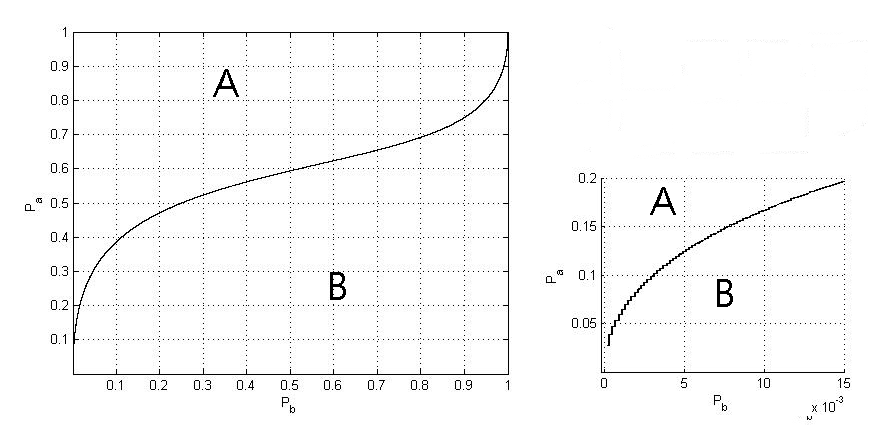

Example 6.
We compare the channel fidelities of the entanglement-assisted (EA) repetition code [14], , and Bowen’s quantum code [21], . Bowen’s quantum code is equivalent to the five qubit code and has , while the EA repetition code is designed under the assumption that Bob’s qubits are perfect and has . We have
and
The channel fidelities of these two EAQEC codes are compared in Fig. 3 and Fig. 4. In Fig. 3, the curve of the boundary between the two regions passes the origin. The region A in Fig. 3 corresponds to the shaded part in Fig. 4. In region B, Bowen’s code is better than the EA repetition code.
In the extreme case of , we have
and
The EA repetition code corrects more lower-weight errors, and hence it has higher channel fidelity.
The channel fidelity of the quantum code depends on the decoding process. If we treat the combination code as an code, its channel fidelity can be computed as Theorem 9. If we use two sequential decoders, it’s different. First, the possible error operators on Bob’s side collapse to logical errors. Each can be obtained from error operators, after the decoding process of the quantum code. If the errors occur uniformly, the decoded errors also occur uniformly. However, this is not the case for the depolarizing channel : the errors on Bob’s ebits occur according to a distribution that depends on the decoding process. We can find the channel fidelity as in Theorem 9, except that the errors on Bob’s ebits follow a new distribution . We will compare the channel fidelities of these two decoding methods in Section VII.
VI.3 Approximation of Channel Fidelity
The number of terms in the formula for channel fidelity over the depolarizing channel is , which grows exponentially in It is difficult even to build a look-up table for decoding when is large. However, it is possible to approximate the channel fidelity efficiently.
The channel fidelity of a quantum code over a depolarizing channel is the probability that the decoder output is correct, which can be lower bounded by
| Pr | |||
or
| Pr | |||
where is the minimum distance of the quantum code. When the depolarizing rate is low (), these bounds are fairly tight and are good approximations of the true channel fidelity. Dong et al. defined an “infidelity” function to characterize the performance of quantum codes [32], which is an approximation of the channel fidelity in the case of .
We can also apply Monte Carlo methods to approximate the channel fidelity [25], especially when the number of physical qubits involved is large. The steps of the simulations are as follows:
- 1.
Fix a depolarizing rate .
- 2.
Randomly generate an error operator according to the probability distribution of a depolarizing channel.
- 3.
Compute the error syndrome and apply the correction operator and decoding operator.
- 4.
If there is no logical error after decoding, is correctable.
- 5.
Repeat steps 2 to 4 times.
- 6.
Output the channel fidelity as the number of correctable errors in the experiment divided by .
Two applications of the Monte Carlo method to the and codes obtained by MAGMA [31] are shown in Fig. 5 and Fig. 6. In Fig. 5, the exact channel fidelity of the code is also plotted, and it can be observed that the simulations quickly converge to the exact channel fidelity. On the other hand, in Fig. 6, only a lower bound of the channel fidelity of the code is given, since computation of the channel fidelity is difficult ( terms in the formula). However, Monte Carlo simulations also converge quickly from to points, which are much less than .
VII Performance analysis
In this section, we compare the channel fidelity of the quantum code with other quantum codes. A comparable standard stabilizer code with and is a stabilizer code, while the smallest quantum code with is a stabilizer code [30]. By Theorem 2, we can obtain a EAQEC code from the . The EAQEC code is also shown as a reference. All the quantum codes above encode information qubit and hence can be compared with no ambiguity. The channel fidelity of these quantum codes are plotted in Fig. 7. For simplicity, the quantum code using a single decoder is treated as a standard stabilizer code, which means that the weight distribution of the syndrome representatives is like a triangle as in Fig. 2.


When , the EAQEC code is the best code for , and quantum code with sequential decoders and the EAQEC code have better performance for . The quantum code with a single decoder has a comparable fidelity to the EAQEC code.
As the ratio of to decreases, the performance of the quantum code and the , EAQEC codes get better. When , the quantum code, using either decoding method, performs better than the EAQEC code and the stabilizer code.When the ratio of to is below in the last two cases, the quantum code is the best choice. The EAQEC code beats the stabilizer code when as expected. From these plots, the quantum codes that have the best performance are the EAQEC code or the quantum code.
Fig. 8 plots the difference () between the fidelity of a single decoder () and the fidelity of two sequential decoders () of the quantum code. For low noise rates sequential decoding is not as good; however, it is easier to be implemented. Note that, in the simulations, the syndrome representatives using a single decoder are chosen for the same error probabilities on Alice’s and Bob’s qubits. The channel fidelity of the combination using a single decoder will be better if we optimize it over the choices of the syndrome representatives according to the different error probabilities.
VIII EAQEC and Entanglement Distillation
Up to now, we have assumed that Alice and Bob have perfect ebits before the communication, and any noise results from storage errors. In a more general situation, the exchange of perfect maximally-entangled states might not be possible, and entanglement distillation is needed. Our next direction is to find good strategies against this problem.
We first introduce the entanglement distillation protocol. Suppose Alice has the ability to prepare pairs of maximally-entangled states (Bell states)
where is the binary representation of the numbers between and . The state has the following property.
Lemma 11.
For any operator on an -qubit maximally entangled state,
where is the transpose of .
Suppose Alice uses an stabilizer code defined by a stabilizer group with generators , and is a set of syndrome representatives corresponding to . Let be a Clifford encoder of the stabilizer code, and for be the logical states. The encoded is
We know that and is a set of orthonormal basis vectors of . In the case of , we have
If , Alice applies the operator on half of the ebits. From Wilde’s encoding circuit algorithm [33], an encoding operator can be implemented by a series of Hadamard gates, CNOT gates, SWAP gates, and phase gates. If phase gates are not used in the circuit, the circuit will satisfy .
Alice sends half of the ebits to Bob through a noisy channel with depolarizing rate equal to . The corrupted state is
After performing a syndrome measurement, Alice obtains a syndrome , which is a binary -tuple, and she sends to Bob through a noiseless classical channel. Now the state is
where is the syndrome representative of . Let be the error syndrome of . Bob measures the stabilizer generators and obtains the syndrome
The error syndrome can be retrieved by . He applies the correction operator and obtains the state
Finally, they restore the state to the standard encoded state by applying the operator , followed by the decoding circuit and obtain the state
if is correctable. This is called an entanglement distillation protocol. Let denote the combination of the above processes. The entanglement fidelity [23] of this protocol is
The entanglement fidelity of the entanglement distillation protocol when the channel is the depolarizing channel is just the channel fidelity of the corresponding stabilizer code over the depolarizing channel .
After performing an entanglement distillation protocol that produces ebits with some entanglement fidelity, Alice can use an EAQEC code to send information qubits to Bob. Assume and for simplicity. The channel fidelity from the combination of an entanglement distillation protocol and an EAQEC code is similar to that of a combination code using two sequential decoders. On the other hand, Alice could directly use an EAQEC code with the imperfect ebits to send information qubits to Bob without entanglement distillation. The channel fidelity of this process is just the channel fidelity of the EAQEC code.
Example 7.
Alice and Bob use an entanglement distillation protocol to produce 3 perfect ebits from 8 noisy ebits. Then Alice can use an EAQEC code to send quantum information to Bob. Or she can instead use a EAQEC code with the 8 corrupted ebits. Comparison of the channel fidelity of these two schemes is shown in Fig. 9.

Example 8.
Alice and Bob use a entanglement distillation protocol to produce 1 perfect ebit from 5 noisy ebits. Then Alice can use a EAQEC code to send quantum information to Bob. Or she can instead use a EAQEC code with the 5 noisy ebits. Comparison of the channel fidelity of these two schemes is shown in Fig. 10.

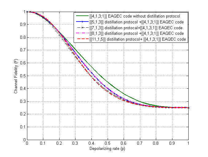
In Fig. 11, we plot the channel fidelity of four distillation protocols with the same EAQEC code. The channel fidelities of the 4 schemes with distillation protocols are better than the one without distillation protocol for , but the difference is small. The EAQEC code without distillation dominates the performance for higher .
In Fig. 12, we plot the channel fidelity of several coding schemes that encode information qubit. It can be observed that the EAQEC codes without distillation protocols have better performance for .

IX Discussion
In this paper, we proposed two coding schemes for EAQEC codes when the ebits of the receiver suffer errors. In the first case we assume the ebits suffer storage errors. EAQEC codes that are equivalent to standard stabilizer codes have better performance than their corresponding stabilizer codes. Several such EAQEC codes are found to achieve the linear programming bound, and hence are optimal. However, as long as the storage error rate is small enough, a quantum code with two encoders performs well if we start with an EAQEC code that is not equivalent to any standard stabilizer codes. We may choose the best quantum code according to the noise channel rate and the storage error rate in real situations.
Any (nondegenerate) standard stabilizer code can be transformed into an EAQEC code by Theorem 2. Families of quantum codes, such as quantum Reed-Muller codes [34], quantum BCH codes [35, 36], quantum cyclic codes [37, 38], can be transformed into families of EAQEC codes. It is possible to construct EAQEC codes with a large number of information qubits but a small number of ebits that outperform standard codes.
We developed a formula for the channel fidelity over the depolarizing channel, and used it to evaluate the performance of a variety of quantum codes. For large codes, the channel fidelity cannot be calculated exactly, but can be lower-bounded or approximated by Monte Carlo simulations. A similar formula for the channel fidelity can be developed for other channels with only Pauli errors.
We also compared EAQEC codes combined with entanglement distillation protocols to EAQEC codes designed to tolerate noisy ebits. It seems that EAQEC codes that can correct errors on both the qubits of sender and receiver can have better performance than the codes combined with an entanglement distillation protocol, at least for modest noise rates. For particular combinations of error rates and applications, it should be possible to optimize the choice of code to maximize the fidelity. This optimization is the subject of ongoing research.
Acknowledgements.
TAB and CYL acknowledge useful conversations with Igor Devetak and Mark Wilde. This work was supported in part by NSF Grants CCF-0448658 and CCF-0830801.References
- [1] P. W. Shor, Phys. Rev. A 52, 2493 (1995).
- [2] A. M. Steane, Phys. Rev. Lett. 77, 793 (1996a).
- [3] A. M. Steane, Phys. Rev. A 54, 4741 (1996b).
- [4] A. Ekert and C. Macchiavello, Phys. Rev. Lett. 77, 2585 (1996).
- [5] C. H. Bennett, D. P. DiVincenzo, J. A. Smolin, and W. K. Wootters, Phys. Rev. A 54, 3824 (1996a).
- [6] E. Knill and R. Laflamme, Phys. Rev. A 55, 900 (1997).
- [7] A. R. Calderbank, E. M. Rains, P. W. Shor, and N. J. A. Sloane, Phys. Rev. Lett. 78, 405 (1997).
- [8] D. Gottesman, Stabilizer codes and quantum error correction, Ph.D. thesis, California Institute of Technology, Pasadena, CA (1997).
- [9] A. R. Calderbank and P. W. Shor, Phys. Rev. A 54, 1098 (1996).
- [10] A. M. Steane, Proc. R. Soc. London A 452, 2551 (1996c).
- [11] A. R. Calderbank, E. M. Rains, P. W. Shor, and N. J. A. Sloane, IEEE Trans. Inform. Theory 44, 1369 (1998).
- [12] M. A. Nielsen and I. L. Chuang, Quantum Computation and Quantum Information (Cambirdge University Pressr, Cambridge, UK, 2000).
- [13] T. Brun, I. Devetak, and M.-H. Hsieh, Science 314, 436 (2006).
- [14] C.-Y. Lai and T. A. Brun, (2010), arXiv:1008.2598.
- [15] M. M. Wilde and M.-H. Hsieh, (2010a), arXiv:1010.1256.
- [16] M.-H. Hsieh, T. A. Brun, and I. Devetak, Phys. Rev. A 79, 032340 (2009).
- [17] C.-Y. Lai, T. A. Brun, and M. M. Wilde, (2010), arXiv:1010.5506.
- [18] M. M. Wilde and M.-H. Hsieh, in Proceedings of the 2010 IEEE International Symposium on Information Theory (Austin, Texas, USA, 2010) pp. 2713–2717, arXiv:0904.1175.
- [19] M. M. Wilde and D. Fattal, Quantum Information Processing 9, 591 (2010).
- [20] B. Shaw, M. M. Wilde, O. Oreshkov, I. Kremsky, and D. A. Lidar, Phys. Rev. A 78, 012337 (2008).
- [21] G. Bowen, Phys. Rev. A 66, 052313 (2002).
- [22] R. Laflamme, C. Miquel, J. P. Paz, and W. H. Zurek, Phys. Rev. Lett. 77, 198 (1996).
- [23] B. Schumacher, Phys. Rev. A 54, 2614 (1996).
- [24] M. Reimpell and R. F. Werner, Phys. Rev. Lett. 94, 080501 (2006).
- [25] N. Metropolis and S. Ulam, Journal of the American Statistical Association 44, 335 (1949).
- [26] C. H. Bennett, G. Brassard, S. Popescu, B. Schumacher, J. A. Smolin, and W. K. Wootters, Phys. Rev. Lett. 76, 722 (1996b).
- [27] Z. Luo and I. Devetak, Phys. Rev. A 75, 010303 (2007).
- [28] J. Preskill, Lecture Notes on Quantum Computation, 1999, ch. Quantum Error Correction (California Institute of Technology, 1999) pp. 15 – 16.
- [29] D. Bacon, Phys. Rev. A 73, 012340 (2006).
- [30] M. Grassl, “Bounds on the minimum distance of linear codes and quantum codes,” Accessed on 2010-12-01.
- [31] J. J. Cannon and W. Bosma, eds., Handbook of Magma Functions, 2nd ed. (2006).
- [32] Y. Dong, Xiuhao, M. Jiang, Q. Chen, and S. Yu, Phys. Rev. A 79, 042342 (2009).
- [33] M. M. Wilde, Quantum Coding with Entanglement, Ph.D. thesis, University of Southern California (2008).
- [34] A. M. Steane, IEEE Trans. Inform. Theory 45, 1701 (1999).
- [35] M. Grassl and T. Beth, in Proc. X. International Symposium on Theoretical Electrical Engineering (Magdeburg, 1999) pp. 207–212.
- [36] S. A. Aly, A. Klappenecker, and P. K. Sarvepalli, IEEE Trans. Inform. Theory 53, 1183 (2007).
- [37] G. Cohen, S. Encheva, and S. Litsyn, IEEE Trans. Inform. Theory 45, 2495 (1999).
- [38] X. Lin, IEEE Trans. Inform. Theory 50, 547 (2004).