Toric bases for 6D F-theory models
Abstract:
We find all smooth toric bases that support elliptically fibered Calabi-Yau threefolds, using the intersection structure of the irreducible effective divisors on the base. These bases can be used for F-theory constructions of six-dimensional quantum supergravity theories. There are 61,539 distinct possible toric bases. The associated 6D supergravity theories have a number of tensor multiplets ranging from 0 to 193. For each base an explicit Weierstrass parameterization can be determined in terms of the toric data. The toric counting of parameters matches with the gravitational anomaly constraint on massless fields. For bases associated with theories having a large number of tensor multiplets, there is a large non-Higgsable gauge group containing multiple irreducible gauge group factors, particularly those having algebras and with minimal (non-Higgsable) matter.
1 Introduction
F-theory [1, 2, 3] provides a very general and nonperturbative approach to constructing vacua of string theory. In six dimensions, there is a large connected moduli space of F-theory vacua. Branches of this moduli space are described by F-theory on elliptic fibrations over different bases that are complex surfaces. Branches associated with different bases are connected through tensionless string transitions [4, 5, 3]. Over each specific base surface there is a rich space of physical theories with different gauge groups and matter content, characterized by different configurations of 7-branes on associated with different singularity structures in the elliptic fibration over . The geometry of an F-theory model is closely mirrored in the structure of the resulting supergravity theory. For example, the number of tensor multiplets in the 6D supergravity theory from an F-theory compactification corresponds to the topological structure of through . 6D supergravity theories with a general number of tensor multiplets that satisfy anomaly cancellation were originally described in [6, 7]. Much of the study of 6D F-theory models has focused on a simple set of base manifolds with small . In particular, the Hirzebruch surfaces give F-theory models with that are dual to heterotic compactifications on a smooth K3 [3]. Recent work [8, 9, 10] has explored the set of models over the simplest F-theory base , with . In this paper we explore the space of all F-theory bases by explicitly constructing and enumerating all smooth surfaces that have a description in terms of toric geometry and can act as bases for an elliptically-fibered Calabi-Yau threefold.
The approach we take here to describing bases for elliptic fibrations is based on the intersection structure of divisors on the base. In a general F-theory model, the gauge group and matter content of the corresponding supergravity theory are determined by the structure of the elliptic fibration. This structure is encoded physically in the positions of 7-branes on . Elliptic fibrations can be described through a Weierstrass model , where are sections of certain line bundles over the base . By varying the continuous parameters in and that describe the fibration, the 7-branes can be moved to increase or decrease the gauge group and massless matter content, corresponding to Higgsing and unHiggsing fields in the supergravity theory. For many bases, such as the Hirzebruch surfaces , the Weierstrass coefficients and must vanish on certain codimension one cycles (divisors) on the base . This gives rise to a certain gauge group content for each base that cannot be removed through Higgsing by massless matter fields in the theory. In a recent paper [11], we gave a systematic analysis of the intersection structure of divisors for any base. We identified a set of irreducible blocks (“non-Higgsable clusters”) composed of one or more intersecting divisors of self-intersection -2 or less that impose a non-Higgsable gauge group, sometimes combined with a fixed massless matter representation, on the resulting supergravity theory. In this paper we use this set of blocks as a guide in the construction of all toric bases. For toric bases, the configuration of irreducible effective divisors with negative self-intersection is very simple, and always lies within a closed linear chain, greatly simplifying the analysis. A challenge for future work is to use related methods to analyze more general, non-toric bases. Previous work has been done using toric geometry in another way to classify elliptically fibered threefolds for F-theory compactifications [12, 10]. In that work, toric methods were used to construct the entire threefold for the compactification as a hypersurface in a toric variety (compact Calabi-Yau manifolds cannot themselves be toric). The approach taken here simplifies the story by focusing on the geometry of the base.
For a given toric base, the methods of toric geometry give a simple classification of the monomials that appear in the Weierstrass coefficients . This gives an explicit Weierstrass parameterization for every toric base. We clarify some subtleties in the counting of degrees of freedom and confirm that the number of degrees of freedom in the Weierstrass models matches with the number of massless scalar fields expected from the gravitational anomaly condition , where is the number of vector multiplets. This explicit parameterization can be used for further analysis of the space of theories over any given base. It also confirms for any given base that the minimal gauge and matter content is precisely that expected from the non-Higgsable clusters in the set of irreducible divisors.
In Section 2 we review some basic aspects of F-theory, algebraic geometry, and toric geometry that will be useful. In Section 3 we describe the complete set of toric bases for 6D F-theory models. In Section 4 we show how an explicit Weierstrass parameterization can be easily constructed for any toric F-theory base, and describe how the number of degrees of freedom in the theory matches the toric data. Section 5 suggests natural extensions of this analysis to non-toric bases and four-dimensional F-theory models, and Section 6 contains concluding remarks.
2 Geometry of bases for 6D F-theory models
In this section we briefly review some aspects of F-theory and geometry that will be useful in this work. Some of the basic aspects of the ideas used here are described in more detail in [11]. Further pedagogical introductions to F-theory can be found in [13, 14, 15].
2.1 Base surfaces for F-theory models
A six-dimensional F-theory model is constructed from an elliptic fibration with section over a base , where the total space is a Calabi-Yau threefold. The elliptic fibration for a 6D F-theory model can be described by a Weierstrass form
| (1) |
Here and the discriminant locus
| (2) |
are sections of line bundles
| (3) |
where is the canonical class of . The intersection form on controls much of the physics of the associated 6D supergravity theory [16, 17]. This intersection form has signature , where is the number of tensor multiplets in the 6D supergravity theory. The discriminant locus can be described physically in terms of 7-branes in the language of type IIB string theory [18]. These 7-branes are wrapped on divisor classes where vanishes. Singularities of the elliptic fibration can occur where the Weierstrass coefficients and vanish. Such codimension one singularities were classified by Kodaira [19] and correspond to a nonabelian gauge group in the 6D supergravity theory, the algebra of which can be computed using the Tate algorithm [3, 20, 21, 22]. The type of singularity on a curve is determined by the degrees of vanishing of on that curve. For example, when and vanish to orders 4 and 5, vanishes to order 10 and the singularity gives rise to an gauge algebra. When vanish to order and , vanishes to order 12 and the singularity cannot be resolved in a fashion compatible with the Calabi-Yau condition on the total space of the fibration. Tables of singularities and symmetries are found in many F-theory papers and reviews, including [3, 20, 22, 11].
When contains an irreducible effective divisor of self-intersection or below, and must vanish on to at least order 2, and a nonabelian gauge theory must appear in the corresponding 6D supergravity theory. In general this situation is described by the “Zariski decomposition” of [23, 24], where any effective divisor can be decomposed over the rational numbers as
| (4) |
where (the “free part”) satisfies for all curves on the surface and for the irreducible effective such that , and (the “fixed part”) contains all irreducible divisors with . For example, for a curve of self-intersection , the Zariski decomposition of the anti-canonical divisor is , so sections of must vanish at least twice ( times) on , and thus must carry a gauge group the algebra11 1 Because the gauge group can have a quotient by a discrete subgroup, it is more precise to state this condition for the algebra, rather than for the group. of which contains . Similarly, a divisor of self-intersection must carry an , and for various other gauge algebras must appear, up to curves of self-intersection that carry an gauge algebra. Furthermore, certain combinations of intersecting curves with negative self-intersection must carry more complicated gauge group factors with charged matter. For example, a curve intersecting a curve must carry a gauge algebra and charged matter living in the representation of this algebra. A complete analysis of all such possibilities is given in [11]; the results of this analysis are summarized in Table 1, with the associated geometries depicted in Figure 1. The clusters with a single curve of negative self-intersection are all familiar from bases, and the gauge groups and matter content associated with multiple-curve clusters were previously encountered in the field theory context in [25]. In addition to the various “non-Higgsable” clusters that must carry a nontrivial gauge group factor and (in some cases) matter, there can also be configurations of intersecting curves. and do not need to vanish on the curves, so there is no gauge group enforced on these blocks. The gauge group over any irreducible curve can have a larger algebra than the minimal algebra indicated in Table 1, if the Weierstrass coefficients vanish at higher order then the minimal order required. In general, however, such larger gauge groups can be broken by Higgsing massless matter fields, and for generic Weierstrass coefficients over any given base the gauge algebra and matter content are expected to have the minimal form. We do not have a proof that this is true in general, but, as described in Section 4, this property holds for all the toric bases constructed in this paper.
| Diagram | Algebra | V | matter | |||
| 0 | 1/3 | |||||
| 0 | 1 | |||||
| 0 | 16/9 | |||||
| 0 | 8/3 | |||||
| 56 | 57/16 | |||||
| 0 | 9/2 | |||||
| 0 | 25/3 | |||||
| 3/8 | ||||||
| 17 | 5/12 | |||||
| (1, 1, 2 ) | ||||||
| 27 | 1/2 | |||||
| (1, 2, 3) |
The various clusters described in Table 1 can be connected by curves that intersect multiple clusters in various ways. The details of which clusters can be connected by curves are described in [11]. There can also be connected sets of curves connected to each other and the irreducible clusters by curves.
While a codimension one locus in the base where vanishes to order 12 cannot be made compatible with a resolved elliptic fibration where the total space is a Calabi-Yau threefold, the same is not true of a codimension two singularity locus. If the degrees of vanishing of reach at a point in the base, it is still possible to resolve the geometry to get a valid F-theory compactification. This requires, however, that the point in the base is blown up, associated with an extremal transition to another base geometry . Blowing up a point in modifies the space of divisors and the corresponding intersection form in a simple way described by standard results in algebraic geometry [26, 27]. In general, blowing up a point in the base gives a new rational curve with the topology of . This curve is a new irreducible effective divisor (the “exceptional divisor”) with self-intersection . The blow-up is described generally by a map where . Any curve with self-intersection in that passes through with multiplicity goes to a curve in (the proper transform of ) with self-intersection and . The anticanonical divisor of contains as a component
| (5) |
where denotes the total transform, i.e., the proper transform of a that does not pass through . The results of blowing up a point on one of a set of intersecting irreducible effective curves are shown graphically in some simple cases in Figure 2. Blowing up a point on a curve leads to a curve with self-intersection crossed by the exceptional curve. Blowing up a point at an intersection between a curve and a curve gives a chain of three curves of self-intersection , with the exceptional divisor in the middle. These are the only cases needed in the analysis of toric varieties that we focus on in this paper. More generally, the geometry can be more complicated with multiple intersections between divisors and singularities such as nodes on the divisors. We touch on these issues briefly in Section 5.1
2.2 Toric bases
Toric varieties are a particularly beautiful and simple class of algebraic varieties. A toric variety is essentially an algebraic variety carrying an action of , where is the complex dimension of the variety. Toric varieties of complex dimension can be thought of as different compactifications of . We only use the very basic aspects of toric geometry in this paper. A good introduction to the subject can be found in [28], and in various papers such as [29] that emphasize the application to physics.
We give here a brief review of the elements of toric geometry needed for understanding toric varieties of complex dimension two, or toric surfaces, following [28]. A toric surface is defined by a fan consisting of a set of one-dimensional and two-dimensional cones emanating from the origin 0 of the 2D lattice . The 1D cones are rays generated by integral vectors , with no two vectors parallel. The 2D cones are the regions between adjacent rays (which must be convex). The origin is a zero-dimensional cone that is also included in the fan. The origin represents the complex torus , which is contained in every toric variety, 1D cones represent divisors, and 2D cones represent points, with the geometric picture of inclusions for the manifold matching that of the toric diagram although dimensions are inverted.
The set of holomorphic functions on the set associated with the origin of is . A holomorphic monomial is associated with every element of the dual lattice Hom (). Choosing a specific basis for , the element is associated with the monomial . For every cone in the fan there is a ring of holomorphic functions that extend to the part of the variety associated with that cone. This ring is described by the dual cone . This gives a set of local coordinate patches that can be glued together giving a global algebraic description of the variety. The surface is compact when the fan covers the entire plane — i.e., when the 2D cones are taken between all pairs of vectors in a cyclic ordering. The surface is smooth if the vectors bounding each 2D cone form a basis for the lattice.
As a simple example, the fan for is generated by the vectors
| (6) |
The holomorphic functions on the torus are spanned by monomials , with . For the cone spanned by the dual cone is spanned by so in that coordinate patch local holomorphic functions are , generated by . In the patch associated with the cone spanned by the holomorphic functions are generated by , and in the cone spanned by the holomorphic functions are generated by . These are the usual local coordinates on in homogeneous coordinates where , with the usual rules for patching together the different local coordinate charts. As another class of examples, the fan for the Hirzebruch surface is generated by the vectors
| (7) |
The Hirzebruch surfaces are bundles over ; this can be seen in the toric description, from the projection along the vertical axis; the vectors provide the fan of the fiber , and the projection of the remaining vectors provide the fan of the base .
The irreducible effective divisors and intersection structure of a toric variety can be read off directly from the toric diagram. The general algorithm for deriving the intersection ring from the toric data is particularly simple in the case of surfaces. On a surface, each vector generating a 1D cone represents an irreducible effective divisor . There are two linear relations on these divisors, given by
| (8) |
for . Each pair of adjacent divisors has an inner product . For a smooth surface, each vector satisfies for some ; the self intersection of the corresponding divisor is . The negative of the canonical class of any toric variety is given by the sum of divisors associated with all
| (9) |
For example, for the Hirzebruch surfaces the linear relations give and as the generators of the cone of effective divisors (Mori cone), where is a fiber and is the section of the elliptic fibration, with . The irreducible effective divisor is a generic section with . The canonical class for the Hirzebruch surfaces is .
The set of irreducible effective curves associated with the toric divisors can be described graphically as a loop of connected curves, as shown in the right side of Figure 3 (see also Figure 6). For the toric surface to be a good base for an F-theory compactification, the sequence of intersection numbers must correspond to an allowed sequence of blocks from Table 1 connected by curves of self-intersection or less. In [11] a complete analysis is given of which blocks can be connected by a curve of self-intersection . The results of this analysis relevant for toric surfaces are summarized in Table 2. For example, a curve can be connected to another curve by a curve, but not to a curve as the degrees of vanishing of become too great at the intersection of the and curves, so that point must be blown up to get an acceptable F-theory base. These connectivity rules provide strong constraints on which toric surfaces can be used as F-theory bases.
| Cluster | Possible subsequent clusters |
|---|---|
| (-12) | (-2, -2, -3) |
| (-8) | (-2, -3, -2) or below |
| (-7) | (-2, -3, -2) or below |
| (-6) | (-3) or below |
| (-5) | (-3, -2, -2) or below |
| (-4) | (-4) or below |
| (-3, -2, -2) | any cluster |
| (-3, -2) | (-8) or below |
| (-3) | (-6) or below |
| (-2, -3, -2) | (-8) or below |
| (-2, -3) | (-5) or below |
| (-2, -2, -3) | (-5) or below |
| (-2, -2, …, -2) | any cluster |
A point represented by a 2D cone bounded by 1D cones generated by can be blown up by adding a new vector to the fan, and dividing the 2D cones accordingly. Similarly, a curve represented by a vector which is equal to the sum of the adjacent vectors is always a curve and can be blown down. For example, as described in (6) can be blown up at the point in the cone bounded by giving the point , reproducing the toric description (7) of . Since admits a symmetry which maps any point to any other, this is the only blow-up of . For each , there are two possible blow-ups. We can blow up the cone , adding the vector or we can blow up the cone , adding the vector . (Note that blowing up the cones give equivalent results after a redefinition of lattice basis). The blow-up of corresponds to the blow-up of at a generic point, while the blow-up of corresponds to blowing up at a point on the divisor associated with , which satisfies . The results of blowing up an in either way describe a class of surfaces , with toric generators
| (10) |
Thus, blow-ups connect to and . These blow-ups are shown in both toric and graphical curve form in Figure 4.
3 Enumeration of bases
The mathematical classification of complex surfaces is well understood [27, 30]. In the minimal model approach, a surface is systematically reduced by blowing down curves until a minimal surface without curves is reached. Using this approach, all smooth F-theory bases giving 6D supergravity theories can be blown down to or by successfully blowing down irreducible effective curves [31, 3].22 2 The Enriques surface is also a possible F-theory base; this branch gives rise to a theory with no gauge structure or matter content. (Note that the Enriques surface cannot be further blown up without destroying the Calabi–Yau property of the total space of the elliptic fibration.) It may also be possible to make sense of F-theory on base spaces with orbifold singularities [3]; we do not consider such bases here. Note that after blowing down an F-theory model, the Weierstrass model on the blown down surface has of multiplicities at least at the blown down points, which is why we normally study these models in blown-up form.
This minimal model result implies that all smooth toric F-theory bases can be reached by starting with or and successively blowing up points at the intersection between adjacent divisors to generate bases with increasing values of . After a sequence of such blow-ups, only those bases described by a sequence of intersection numbers that is built from clusters listed in Table 1 connected by curves of self-intersection or greater with the connections obeying the rules in Table 2 are possible. We have systematically enumerated all possible toric bases for 6D F-theory models using this approach. The computational details of this calculation are described in the Appendix. The result is that we find 61,539 distinct smooth toric bases possible for 6D F-theory compactifications. Some of these toric bases contain or curves with additional singularities that must be blown up where they cross the discriminant locus. While these bases are not technically toric after this blow-up, they have a closely related structure and we include them in our analysis; we discuss this point further below. Taking a strict definition of toric bases, by not including the bases with these types of curves, reduces the total number of bases to 34,868, with the largest value of being 129. The values of for the allowed bases range from and with respectively, to a base with , where in the last case the toric base has two curves that are blown up, as discussed further in Section 3.2.
3.1 Distribution of bases, non-Higgsable gauge groups, and matter content
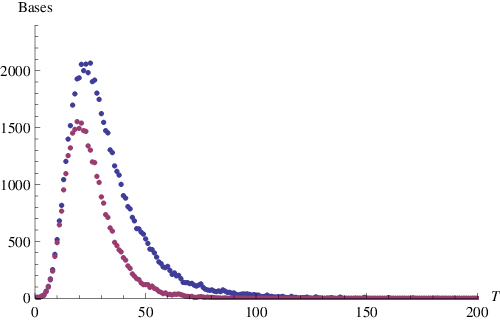
The number of bases identified for each possible number of tensor multiplets is graphed in Figure 5. The numbers of bases for some representative values of are listed in Table 3. For the bases are , the Hirzebruch surfaces and the surfaces described above. (Note that the Hirzebruch surfaces contain singular points that must be blown up for a good F-theory base at , so that there are only 10 good F-theory bases at .) The largest number of distinct bases appears at , where there are 2066 distinct toric bases. The range of bases rapidly drops between 30 and 60, and is the smallest value of with no allowed toric bases. The bases become more sporadic up to the maximum of . Some details of the bases with large are discussed in the following subsection.
| 0 | 1 | 2 | 3 | 4 | 5 | 6 | 10 | 20 | 25 | 30 | 50 | 100 | 150 | 193 |
| 1 | 10 | 10 | 21 | 31 | 63 | 106 | 517 | 1937 | 2066 | 1622 | 522 | 29 | 2 | 1 |
A fairly typical33 3 Note, most bases at have at least one divisor of self-intersection or less, so this is not a completely typical base. base at is depicted in Figure 6, both in toric fan and graphical curve form. Any toric base is characterized simply by the sequence of self-intersection numbers of the irreducible effective curves that form a closed loop. From the clusters of curves with self-intersections below we can read off the non-Higgsable gauge algebra content of the supergravity model associated with any such base. For example, for the base depicted in Figure 6 the gauge algebra is
| (11) |
One subtlety, noted above, is that many of the toric bases reached after blowing up a sequence of points on a surface contain curves of self-intersection and . In these cases, as mentioned in [11], points on these curves must be blown up for a good F-theory model. Specifically, the degree of vanishing of the discriminant locus on is given by from . Similarly, the degrees of vanishing of are . (This can easily be read off from the Zariski decomposition given above.) The residual part of the discriminant locus has a further intersection with of multiplicity . Writing the equation of the curve as , we see locally that , so . It follows that the residual discriminant locus has a factor of and is locally tangent to . At these intersection points the degree of is increased to 12, so the points must be blown up. After blowing up these points we have curves of self-intersection that carry an gauge algebra without matter. Physically, this resolution arises because there is no appropriate representation for matter charged under the where it intersects the residual curve. While the bases that result from this process are not actually toric, due to the final blow-ups on the or curves, the structure of these bases is closely related to that of the toric bases and we include them in our analysis, associated with the value of that results after the necessary blow-ups of the or curves. In the remainder of this paper we use the term “toric base” loosely to include both the genuine toric bases and those where and curves on a toric base have been blown up.
In other work, another approach has been taken to understanding elliptically fibered Calabi-Yau threefolds for 6D theories from toric geometry. Many Calabi-Yau threefolds can be realized as hypersurfaces in toric varieties of one higher dimension, with a simple description in terms of reflexive polyhedra using the Batyrev construction [32]. In [12], threefolds for 6D F-theory compactifications were analyzed from this approach and a method was given for computing the gauge group and number of tensors from the toric data. Kreuzer and Skarke [33] have systematically identified the roughly 500 million reflexive polytopes in four dimensions. In principle, one could identify all toric elliptic fibrations for F-theory from among this list. Recently, Braun [10] has identified those reflexive polytopes that correspond to elliptic fibrations over . By focusing on the structure of the base, the analysis we have used here simplifies the problem of identifying the distinct possible F-theory bases. For each base, there will be many elliptic fibrations in which the gauge group is enhanced, with a wide range of matter structures coming from different types of codimension two singularities. Braun identified 102,581 elliptic fibrations over . Some of the range of possible matter representations that can appear in 6D F-theory models over are identified from anomaly constraints in the low-energy supergravity theory in [8], and analyzed from the point of view of codimension two singularities in F-theory in [9]. Understanding and classifying more completely the range of structure possible over a given base such as is an interesting problem for future work. For each of the 61,539 toric bases we have found, there will be a similar broad class of constructions. As increases, however, the number of available moduli to tune additional gauge groups decreases, as we discuss in Section 4. Thus, we expect that while there are many models at larger values of , the range of possibilities for enhanced gauge groups and matter structure will decrease as increases. An interesting project for future work would be to relate the set of bases found here by direct toric analysis of the base surface to those bases that appear in the elliptic fibrations from the Kreuzer and Skarke database.
3.2 Bases with large
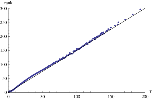
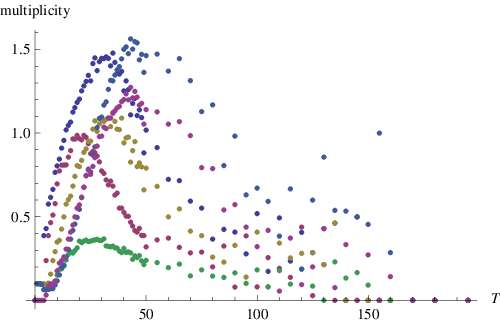
As the complexity of the bases increases with , the minimal (non-Higgsable) gauge algebra associated with the bases becomes larger. In Figure 7 we show the average rank of the gauge group as a function of . The rank grows roughly linearly with , with a slope close to . To understand this it is helpful to consider the more detailed structure of toric bases at large . In Figures 8 and 9 we graph the average number of each of the non-Higgsable gauge algebra summands as a function of . As increases, the gauge algebra is dominated by and summands. The reason that these algebra components dominate can be understood from several aspects of the analysis given in [11]. In that paper we identified a bound on for any theory with a given non-Higgsable gauge group. For theories where the gauge group can be fully Higgsed, is less than or equal to 9. Each gauge algebra summand contributes to the upper bound a quantity given by the last column in Table 1. Thus, for example, a theory with gauge group can have a value of that is at most . As discussed in [11], for most of the combinations of gauge algebra summands that appear in linear chains that can be blown down without “breaking” (reducing to sequences containing multiple curves with self-intersection and no curves), the bound on is relatively low. By blowing up a sequence of curves, however it is possible to generate a periodic sequence of the form
| (12) |
This sequence gives the largest possible contribution to per unit length of any allowed periodic sequence. It is natural therefore to expect that this sequence will play an important role in toric bases at large . Indeed, the toric bases with large are described by sequences of curves dominated by this periodic pattern. This corresponds in Figure 9 to the fact that the number of and summands grows as while the number of summands grows as at large . Similarly, the rank contribution from each iteration of this pattern is 18, which with increasing by 12 reproduces the observed 3/2 slope seen in Figure 7.
The largest toric base has 194 curves corresponding to the rays in the toric fan. The self-intersection numbers of these curves are essentially 16 repeated copies of (12) with a on each end, and a curve of self-intersection 0 closing the loop. The actual toric base has two curves in the next-to-last places for curves. As discussed at the end of the previous section, these must be blown up, so that the final associated F-theory base is not strictly toric and has curves intersecting the second and penultimate ’s in the chain. The resulting geometry of the F-theory base gives the 6D supergravity theory with the largest gauge group rank known, previously identified in [12, 34]. This F-theory base has and gives a theory with the largest number of tensor multiplets known for any consistent 6D supergravity theory. One way to reach this geometry is to start with , blow up the intersection point between the divisor () and a particular fiber 24 times, and then blow up points on that fiber, leaving another fiber as the -curve that closes the loop. Another possibility is to start with , and then blow up the intersections connecting the curve with two different fibers 6 times each, and then blow up points on the two fibers, leaving as the -curve that closes the loop. The first of these possibilities can be described in terms of the systematic algorithm used for constructing all toric bases in the Appendix, and was used in [34] to construct the base geometry with .
As the number of tensors approaches the maximum of for toric models, bases appear only sporadically. The next-highest value of where there is a toric base is , where there are two possibilities. These bases have essentially the same structure as the base, but only 15 copies of the cycle (12), and minor variations on the detailed structure. In one case, the ’s on the end of the sequence are connected by a pair of curves instead of a single curve of self-intersection . In the other case, both the next-to-last and the final on one end of the chain are replaced by ’s that are blown up at one point. At there are four variations on the pattern with 14 copies of the cycle (12). At and below there are bases at most values of , which begin to break the pattern further — the base at for example consists of 12 copies of the cycle (12) (with the second coming from a blown-up ), followed by the sequence — the short regular pattern at the end with alternating and clusters corresponds to one of the cyclic linear chains described in [11].
4 Weierstrass models
From the toric description we can readily identify the monomials appearing in the Weierstrass description (1) of the elliptic fibration over any given base. This provides a tool for analysis of the class of models over any given base. It is also illuminating to match the number of degrees of freedom in the Weierstrass model to the number of scalar hypermultiplets expected in the supergravity theory. In this section we describe the details of these calculations and clarify some subtleties in the degree of freedom counting.
4.1 Monomials in toric bases
Just as the set of holomorphic functions associated with a given cone is described by the dual cone , there is a simple toric description of the monomials corresponding to sections of a given line bundle in the local coordinate patch associated with each cone. To describe the monomials in the Weierstrass functions we need to characterize sections of the line bundles . Recall that for a toric variety, the anticanonical divisor is given by the sum of the divisors associated with the vectors . It follows that for a 2D cone generated by the vectors , the condition that a monomial described by a dual vector is a section of is that . This condition can be geometrically characterized in by the condition that must lie in the cone spanned by a pair of generators for the dual cone , with the base of the cone offset by the vector from the origin.
Based on this characterization, we can easily construct the set of monomials in the global Weierstrass description of any toric base. The monomials for the minimal bases and are shown in Figure 10. For the general pattern is that is constrained by a right triangle with base containing points with a slope of on the diagonal, while is constrained by a similar triangle with points on the base. The total number of monomials for is then
| (13) |
This number is computed for each and tabulated in Table 4.
Note that from the available monomials we can immediately check that the degrees of vanishing of and on each divisor are those expected. For example, for the curve on , associated with the vector , it is clear from Figure 10 that there are no monomials with for , so that vanishes to order (but not higher) on that divisor.
4.2 Degrees of freedom and the gravitational anomaly constraint
The spectrum of any consistent 6D supergravity theory must obey the gravitational anomaly constraint [35, 7, 36]
| (14) |
where and are the numbers of massless scalar hypermultiplets, vector multiplets, and tensor multiplets in the theory. The physical degrees of freedom in the Weierstrass coefficients correspond to massless neutral hypermultiplets in the maximally Higgsed 6D theory. Thus, there is a close correspondence between the monomials in determined from the toric data and the spectrum of the theory. Matching these degrees of freedom for the generic model over toric bases gives insight into a number of features of the theory.
In general, there is a redundancy in the Weierstrass parameters associated with the dimension of the automorphism group of the surface . For when , and for (see Table 4). There is additionally an overall scale factor that can be removed from without changing the geometry. Furthermore, in all cases one scalar field is not a deformation in but rather arises from the overall Kähler modulus of the F-theory base. Finally, as discussed further below, curves of self-intersection that do not live in clusters carrying a gauge group arise at codimension one points in the moduli space, so the degree of freedom removing these curves does not appear in the Weierstrass degrees of freedom for a given base. Putting these contributions together, the number of Weierstrass monomials is related to the number of hypermultiplets in a maximally Higgsed model over any F-theory base through
| (15) | |||||
where is the number of curves on the base that are not in a cluster carrying a gauge group, and is the number of non-Higgsable charged matter fields in the generic model over that base.
In looking at different toric models it is helpful to decompose the extra Weierstrass degrees of freedom coming from the automorphism group of the base into contributions from the different divisors. In general, there are redundant Weierstrass degrees of freedom associated with a divisor of self-intersection in the toric fan. This is easily seen from the description of the automorphism group given by Cox [37], in terms of the homogeneous coordinate ring of the toric surface and the associated “polar polytope”. There is a simple combinatorial description of the polar polytope: it is the set of vectors that satisfy for all of the generators of the fan of the toric surface. This polytope is similar to the regions of points graphed in Figure 10, but with a rescaling of the lattice. Each lattice point which is in the interior of a codimension one face of the polar polytope is associated with a one-parameter subgroup of the automorphism group, and these are all independent. (See also [38]). For a curve of self-intersection , since , the corresponding edge of the polar polytope has lattice points, of which are interior lattice points.
For example, for , each curve associated with a divisor in the toric fan has self-intersection 0. Each such curve has a single degree of freedom associated with fixing the position of the curve in the given toric coordinates (for this corresponds to fixing a coordinate , and for this corresponds to fixing a coordinate ). These degrees of freedom are removed when we blow up points on these curves that fix the locations of the proper transforms in the new base . There are also two Weierstrass degrees of freedom present for every toric variety that cannot be removed by blowing up, associated with rescaling of the two toric coordinates . Combining these contributions with the missing degrees of freedom for curves, we write the total number of “extra” Weierstrass degrees of freedom as
| (16) |
The dimension of the automorphism group is the sum of all these contributions except for the missing moduli from curves
| (17) |
To see how this correspondence works in an example, consider the simple case of . In this case we have (see Figure 10)
| (18) |
Thus, there are coefficients associated with independent monomials in the Weierstrass parameters for . Comparing to (14), the generic model over this base has and a completely Higgsed gauge group (), so we expect . This matches with (15) since for .
Another useful case to consider is . As mentioned above, part of the difference between the number of Weierstrass moduli and the number of hypermultiplets arises from curves of self-intersection . In general, a curve of self-intersection that does not connect to a cluster containing other curves of self-intersection or less (and that therefore does not carry a non-Higgsable gauge group factor by Table 1) arises in the branch of moduli space associated with a base without that curve at a locus of complex codimension one. For example, , which is topologically equivalent to , arises on a codimension one locus in the space of . 44 4 This is seen by embedding into as a nonsingular hypersurface of degree two, and taking a limit to a singular hypersurface (which is isomorphic to with the curve blown down). The singularities of that family of surfaces can be resolved simultaneously, giving a family linking and . Thus, we associate with each curve of self-intersection a deficit in the number of degrees of freedom counted by Weierstrass moduli of , as in (15). For , the number of Weierstrass monomials is 250, and the automorphism group has dimension 7, so only 243 degrees of freedom (including the overall scaling factor that compensates for the missing Kähler modulus) are described by the Weierstrass monomials. The remaining scalar field that brings the total to 244 is the one that was tuned to produce the curves.
For each of the Hirzebruch surfaces , it is straightforward to verify that the counting of degrees of freedom matches both with the size of the automorphism group through (15) and with the degrees of freedom associated with specific divisors through (16). In general, there are extra degrees of freedom in , associated with , or from the divisor of self-intersection , 2 from the two -curves, and 2 universal extra degrees of freedom. Note that for , . This counting indicates that the 28 non-Higgsable hypermultiplets (56 half-hypermultiplets) charged under in the 6D supergravity theory associated with this F-theory compactification do not appear as parameters in the Weierstrass model. This makes sense as only neutral scalars should appear as moduli in the Weierstrass form.
| 0 | 1 | 2 | 3 | 4 | 5 | 6 | 7 | 8 | 12 | |
|---|---|---|---|---|---|---|---|---|---|---|
| 244 | 244 | 244 | 252 | 272 | 296 | 322 | 377 | 377 | 492 | |
| 250 | 250 | 250 | 260 | 281 | 306 | 333 | 361 | 390 | 509 | |
| 6 | 6 | 7 | 8 | 9 | 10 | 11 | 12 | 13 | 17 |
4.3 Blowing up points and degrees of freedom
Having checked that the degree of freedom counting matches for the Hirzebruch surfaces , we can perform a sequence of successive toric blow-ups and match the decrease in degrees of freedom to changes in the divisor structure. From the gravitational anomaly constraint (14) or from simple geometric considerations on the local form of the Weierstrass model, we know that generally 29 scalar degrees of freedom are removed when a point is blown up. The number of Weierstrass degrees of freedom lost may differ if curves of self-intersection or are involved, due to the under- or over-counting associated with these divisors. Furthermore, if the non-Higgsable gauge group structure is changed then the number of massless scalars will change accordingly, in correspondence with the gravitational anomaly constraint (14). The change in degrees of freedom from the different kinds of blow-ups, for example blowing up a point between the curve and a curve in the sequence , can in principle be checked by doing a local analysis of the toric geometry using only the nearby relevant divisors. We have done the check directly on the global models, by systematically verifying for all 61,539 toric bases that the matching between Weierstrass parameters and neutral scalar fields works out. This confirms the expectation that in general global models the gauge group and matter content on any non-Higgsable cluster of intersecting divisors is the minimum required from the intersection of the divisors with . As a particular example, the largest base with has a Weierstrass model with 15 monomials, encoding 12 physical degrees of freedom.
It may be instructive to follow an explicit example through a sequence of blow-up operations and confirm that the number of Weierstrass degrees of freedom varies as expected. Figure 11 depicts a sequence of four blow-up operations on . In the toric fan, the following sequence of points is blown up: (red), (blue), (green), (purple). In the resulting sequence of bases , we have the following structure for the gauge algebra and number of Weierstrass degrees of freedom, where for each base indicates the self-intersection numbers of the divisors (always starting with the toric divisor associated with , and with the exceptional divisor at each stage noted in bold)
| (19) | ||||||||
| (20) | ||||||||
| (21) | ||||||||
| (22) | ||||||||
| (23) |
This sequence of blow-up operations and the resulting constraints on the monomials are shown geometrically in Figure 11. In the first step, 31 Weierstrass degrees of freedom are removed. This can be understood as the 29 physical scalars that are traded for the extra tensor, plus two unphysical Weierstrass moduli associated with the first two divisors in , whose self intersections decrease from and to and (i.e., is reduced from 4 to 2). At the next stage again 31 Weierstrass degrees of freedom are removed. 29 of these again are physical scalars, and two are the extra moduli associated with fixing curves in that do not support a gauge group ( goes from 1 to 3). For the base , the model develops a non-Higgsable cluster that requires a gauge group of . For this model we have , a gauge group of dimension , and 8 charged hypermultiplets. The total number of scalar hypermultiplets should be . There are 2 universal extra Weierstrass parameters, (from extra Weierstrass parameters for the curves of self-intersection and , and two missing moduli from the two curves that do not carry gauge groups), so the number of moduli from the Weierstrass counting should be . The maximally Higgsed model over this base has 8 charged scalar hypermultiplets (16 half-hypermultiplets) that cannot be Higgsed, from Table 1. From this counting it is clear that, just as for the matter charged under on a curve, these non-Higgsable charged matter fields do not appear in the Weierstrass parameters for this model. In the final model with base , we have , a gauge group of dimension , and no matter, so we expect . This is in exact agreement with since there are 2 universal extra Weierstrass parameters, and (from extra Weierstrass parameters for the curves of self-intersection and , and two missing moduli from the two curves that do not carry gauge groups). We can furthermore check that in this sequence of models the degrees of vanishing of on the various curves are precisely the minimal values expected. In particular, we can check that the degrees of vanishing of on the curves in are and , as computed in [11], by confirming for example that all monomials in satisfy , etc.
As discussed above in the case of and the blown-up base from (22), charged hypermultiplets associated with non-Higgsable matter content do not appear as Weierstrass degrees of freedom. This makes sense, as Weierstrass degrees of freedom are generally uncharged scalar moduli (with the exception of the redundant unphysical degrees of freedom discussed above). This raises the natural question of where the moduli associated with the non-Higgsable charged hypermultiplets arise in the F-theory description. Geometrically, from the M-theory point of view the charged matter corresponds to additional 2-cycles in the resolved geometry. Like the cycles associated with gauge fields on the 7-branes, however, these M-theory degrees of freedom are not included in the geometrical degrees of freedom in the Weierstrass description of an F-theory model. Another example of this appears when the Weierstrass parameters are tuned to produce an enhanced gauge symmetry on some particular divisor. As discussed in detail in [9] in the case of the base, and in [39] for the bases , the number of moduli that are tuned to produce, for example, an gauge group is given by the dimension of the group, . Thus, at an enhanced symmetry point, the Weierstrass parameters that are fixed become some of the matter fields that are charged under the enhanced gauge group. The total number of fields also increases, however, at the enhanced symmetry locus by the dimension of the group. Thus, extra charged matter fields must be included when degree of vanishing of the divisor locus is enhanced on some particular curve. Physically, this corresponds to extra degrees of freedom occurring when 7-branes become coincident. On coincident 7-branes there are indeed extra fields, scalar fields that live in the adjoint of the gauge group. These are the fields used in [40] to describe additional structure of the Hitchin bundle over the branes in the structure referred to as “T-branes”. It is natural to speculate that in all cases, the additional “missing” charged scalar fields in the Weierstrass model correspond to such fields on the branes. In fact, it should also be noted that the 6D supergravity scalar hypermultiplet fields are quaternionic and each contain four real degrees of freedom. The Weierstrass moduli are complex and only contain two degrees of freedom; the remaining degrees of freedom are contained within the 7-branes and not usually treated within the F-theory context. Associating the extra charged matter fields with fields on the brane as just suggested would naturally complete the counting of degrees of freedom, although a more explicit description of the non-Higgsable charged matter fields in this fashion is desirable. In any case, the usual formulation of F-theory in terms of Weierstrass models does not contain a number of the degrees of freedom of the theory, such as the overall Kähler modulus and these charged moduli and the other gauge degrees of freedom on the 7-branes, that in the 4D context can carry fluxes. At this stage, while F-theory is a useful way of characterizing a general class of nonperturbative string vacua, there is still no systematic formulation that gives a complete description of the corresponding low-energy supergravity theory. Some recent work on a more complete correspondence through M-theory appears in [41]
5 Further directions
5.1 Non-toric bases
A natural extension of this work is to attempt a systematic classification of all F-theory bases without the toric constraint. It has been proven that the number of birational equivalence classes of elliptically fibered Calabi-Yau threefolds is finite [31, 42]. A simple argument based on the Weierstrass parameterization shows that there are a finite number of branches of the F-theory moduli space associated with distinct bases [16]. But there is as yet no systematic classification of all such bases or elliptic fibrations. To extend the classification beyond the toric set, more complicated intersection structures of divisors must be considered. As analyzed in [11], there are strong constraints on what types of intersections can arise. The only ways in which a set of curves of self-intersection can intersect one another are those tabulated in Table 1, and all ways in which a curve can intersect these clusters are listed in [11]. Nonetheless, the combinatorial possibilities become large as the number of tensor multiplets increases, so a systematic classification becomes challenging. One approach is to begin with a bound on . While we believe that the (essentially) toric example described here and in [12, 34] with is the base with the largest value of , this has not been proven. We describe here briefly two approaches that could be taken to bound and/or to systematically classify more general F-theory bases. We leave further elaboration of these ideas to future work.
For toric bases the irreducible effective curves of negative self-intersection form a simple closed loop of pairwise intersections. The main new features that appear in considering non-toric bases are branches, where one curve can intersect 3 or more other curves, and additional loops. We can construct a large family of non-toric bases that have branching and additional loops but that still have enough of the structure of toric surfaces that they can be studied in a controlled fashion. We do this by considering a slightly more general class of blow-ups of the Hirzebruch surfaces . As discussed in the Appendix, the toric surfaces for F-theory can all be constructed by blowing up only the points at which a pair of fibers intersect the sections of self-intersection , or after blowing up such points, further blowing up at intersection points between pairs of curves of negative self-intersection arising from the blow-up of the . We can explore a larger space of bases by simply including more fibers but only blowing up points in the same fashion. In particular, we do not blow up any points that are on a fiber but not at an intersection either between and or , or between two curves of negative self-intersection that lie within . This choice preserves the action on the fibers that is part of the toric action. In general, it is difficult to tell which new curves of negative self-intersection will appear after blowing up a sequence of points, but in this case with a residual action no new curves need to be added other than the exceptional curves from the blow-ups.
We can in principle systematically describe all non-toric bases with the structure just described. We report here on only one simple experiment in this direction, which provides supporting evidence for the conjecture that there are no models with . We have considered possible non-toric bases that can be formed in the class described above by blow-ups on three distinct fibers . We start from and blow up the intersections between the and by times respectively, with each of and . This gives us a “frame” similar to those described in the Appendix but with 3 chains connecting the divisors . This gives some tens of thousands of non-toric models, of which the largest has . The model with is produced by choosing , and has simple chains replacing , and a chain of length 167 for containing 14 copies of the pattern (12) without the terminal ’s, and with the 12th curve from each end having self-intersection instead of . This base is closely related to the structure of the base with the largest , and the other bases of this non-toric type with large are similar. The next-largest has , with or replaced by and only 13 copies of the pattern in . This analysis indicates that there are no local types of branching where one curve connects to three that increase the range of possible ’s. We can understand this geometrically by noting that large is always associated with chains locally dominated by the pattern (12). This follows from the bounds on for any given gauge group studied in [11]. From that analysis, and from the gravitational anomaly bound (14), it is clear that increasing substantially is only possible when the gauge group is large, and and the associated periodic chain sequence provides the largest gauge group for the smallest change in . To do better than the linear sequence of 16 copies of (12) with terminal ’s that forms the basis of the toric model with , somehow the curves carrying the factors would need to be connected in a way that increases the possible while still giving a surface that blows down to a Hirzebruch surface with only one curve of negative self-intersection. From the connectivity rules in Table 2, a curve can only be connected by a curve to a sequence of curves of self-intersection , and this can in turn be connected to a curve of self-intersection at most . This severely limits the range of possible structures incorporating curves. We cannot, for example, have three chains attached to a single curve, or as we blow down the chains the curve would become a curve of positive self-intersection leaving three disconnected components. This is incompatible with the minimal model result that the surface must blow down to a surface with at most one curve of negative self-intersection, unless the original three chains are connected through other curves. In the latter case the original curve plays no role and can be dropped from the analysis. While this is a somewhat heuristic analysis, it gives the flavor of the underlying geometric reason why it is difficult to connect curves in any way that can allow . Combining this with the systematic analysis of non-toric models with three fibers described above seems to give strong evidence that is indeed the largest value of for any 6D F-theory model, even allowing non-toric structure for the base. A rigorous proof of this result would, however, be nice to have.
While the preceding general arguments suggest that the upper bound on is indeed 193, a complete proof of this statement may be somewhat nontrivial due to the combinatorial complexity of the set of possible combinations of intersecting divisors when the toric constraint is relaxed. The number of possible distinct ways that a curve can intersect a combination of non-Higgsable clusters is 183, as shown in [11]. Considering combinations with more than a few clusters leads to a rapid combinatorial growth in possibilities. Nonetheless, using some general principles it may be possible to put a fairly strict bound on , and possibly even to prove the bound . To illustrate how this might work we briefly consider a simplified piece of the problem. The remainder of this subsection is not relevant for the rest of the paper, and the reader not interested in worrying about how to bound for non-toric bases can skip to Section 5.2.
We consider the subclass of F-theory bases that contain only and curves. This corresponds to low-energy supergravity theories with a gauge group and no matter in the maximally Higgsed phase, where is a discrete quotient that will not concern us. From the general arguments in [11] and the value of in Table 1, we know that any theory with a maximally Higgsed gauge group containing only summands has a maximum value of . There are only a few ways in which curves can be connected by curves. From the Table in [11], a curve can only (i) intersect a single curve once, (ii) intersect two distinct curves once each, or (iii) intersect a single curve twice. This limits the range of possibilities, and makes a general argument bounding both and possible without too many combinatorial complications. The basic idea is to consider all possible ways in which a combination of curves can be connected and blown down to a generalized del Pezzo surface containing no curves of self-intersection or below. Note that any surface with with no curves of self-intersection or less that can be blown down to can also be blown down to — since the points blown up on the must lie off the curve — and therefore can be blown down to a generalized del Pezzo. Generalized del Pezzo surfaces have at most . For , a generalized del Pezzo surface has at most -curves, and for the maximum number of such curves is . The generalized del Pezzo surfaces at are rational elliptic surfaces, for which a complete list is known of the possible intersection configurations of curves [44, 45].55 5 Technically, those papers only consider the cases of rational elliptic surfaces with section, and one must also consider the “Halphen pencil” cases as well [46]. But since the Jacobian fibration of a Halphen pencil is a rational elliptic surface with a section, the configuration of non-multiple singular fibers does not change. While the number of curves becomes infinite at , we need only consider a finite subset. For any valid F-theory base containing a realizable configuration of curves there is at least one finite set of curves that can be added to the curves forming a network with the property that all curves needed to blow down to a generalized del Pezzo are present, and that no curves not needed for this blow down are included. Such a network can be depicted schematically as a graph where a set of nodes (the curves) are connected by edges (the curves) (see Figure 12).
If we denote by the number of curves in an allowed configuration on a base associated with a theory having a given value of , the number of blow-downs that must be done to reach a generalized del Pezzo, and the number of curves remaining after the blow-downs, we have from the bound on the number of curves
| (24) |
We can, however, determine a lower bound on the ratio
| (25) |
For any connected graph, this bound holds. For example, a graph formed from a loop of curves connected by curves (Figure 12 (a)) has so . As another example, the graph formed by a single curve connected by curves to 3 other curves (Figure 12 (b)) has , so . The bound is matched by a graph component consisting of a curve connected to 3 other curves of which one is terminal and two connect by a single edge to another graph component — this blows down to a curve intersecting a pair of curves at a single point and has a contribution of (counting the blow-down of each of the two “external” edges as ) for a total of . The simplest example of a graph formed from a single component of this type is shown in Figure 12 (c). This graph has so ; note that the blown-down configuration contains in addition to the curve a pair of curves not shown in the figure, which intersect each other in two points, one of which is along the curve. A somewhat tedious case-by-case analysis of various components shows that the bound (25) cannot be exceeded. (For example, extending any diagram by including an extra node on a linear string of nodes contributes a factor of just as in the closed loop example above). From (25) and (24) it follows that , from which it follows that for any F-theory base corresponding to a 6D supergravity theory with only gauge algebra summands. This shows how in principle can be bounded for a given class of gauge algebras. In fact, this bound is weaker than the true limit. The configurations that realize the bound (25) give curve configurations that cannot appear in a generalized del Pezzo with [44, 45]. It seems likely that the maximum that can be realized in practice is . This can be achieved by a set of loops as in Figure 12 (a) of total length 12, or 3 copies of Figure 12 (b). Note that a loop of this type of length 12 is not possible. One possible configuration of total length 12 comes from an allowed configuration of curves on consisting of nine curves in a closed loop and three curves in a closed loop of length one (i.e., with a single self-intersection). It is not possible to achieve a closed loop of alternating curves in the toric context since this would blow down to a closed loop of curves, not a Hirzebruch surface. The largest related toric base without curves of self-intersection or below has a loop of curves containing six curves and three curves in 3 repeated copies of the pattern . Non-toric blow-ups of the 3 curves give a loop containing nine curves with the structure of Figure 12 (a). Note also that while 4 copies of the diagram in Figure 12 (b) does not violate the bounds stated above, the detailed list of possible configurations on a rational elliptic surface only allows for three of the Kodaira type IV configurations of three intersecting curves. In principle such constraints can be included in a stricter bound that seems likely to rule out all configurations with , but we do not pursue the details of such an argument here. This discussion is intended only to give a flavor of how one might construct a general argument bounding , where a much more complicated set of configurations involving all the possible clusters from Figure 1 must be treated. We leave further analysis along these lines for future work.
5.2 Constraints on 6D supergravity theories
In ten dimensions, the macroscopic conditions of supersymmetry and anomaly cancellation conditions constrain supergravity theories so strongly that all spectra compatible with these conditions are realized as string theory vacua [47, 48, 49]. A theme in a series of recent works has been to investigate the extent to which a similar statement is true in six dimensions by exploring the space of 6D theories compatible with known constraints [50, 51, 39, 52]. F-theory, in its current formulation, imposes additional constraints on 6D supergravity theories; because of the close correspondence between 6D supergravity data and F-theory geometry, these F-theory constraints can be interpreted in a straightforward fashion as conditions on the spectrum and action of 6D supergravity theories [16]. One constraint imposed by F-theory on 6D supergravity is that the lattice of dyonic string charges in the 6D theory be unimodular. This turns out to be a consistency constraint on 6D supergravity theories independent of F-theory [17], and therefore limits the space of theories. Other constraints arise from F-theory for which it is not yet known whether the constraints are actually necessary for consistency of quantum supergravity KEK in 6D, or if the constraints are simply associated with F-theory and can be avoided in another approach to quantum gravity, such as a more general string compactification mechanism. One such constraint on the low-energy theory follows from the “Kodaira condition” in F-theory stating that the total discriminant locus is [16]. In the low-energy theory, appears in the gravitational Green-Schwarz coupling of the form , where , and the divisor classes on which 7-branes are wrapped to give nonabelian gauge groups are encoded in the gauge Green-Schwarz couplings of the form , where . These terms are constrained by the Kodaira condition since must be an effective divisor (where is the multiplicity of 7-branes wrapped on ) and therefore the corresponding combination of Green-Schwarz coefficients must give a certain sign when dotted into the Kähler modulus , which is a vector under associated with the scalars in the tensor multiplets.
In the analysis of [11] and this paper, we used a key feature of the algebraic geometry, which is that whenever there exists an irreducible effective divisor with , it is necessarily the case that and there must be a nonabelian gauge group factor associated with this divisor. This condition has a corresponding interpretation in the resulting low-energy supergravity theory. For any low-energy 6D supergravity theory arising from F-theory, if there is a supersymmetric dyonic string state of charge such that the inner product associated with Dirac quantization satisfies , then must be the coefficient in a Green-Schwarz coupling for some gauge group factor containing at least the minimal gauge algebra associated with that negative self-intersection number through Table 1. This is true as well for the combinations of self-intersection numbers , etc. giving non-Higgsable clusters containing multiple divisors. This condition is a highly nontrivial constraint on 6D supergravity theories, relating the structure of the dyonic string spectrum to the gauge and matter structure of the theory. This condition is also sufficient to imply the Kodaira condition. It would be very interesting to identify some reason in low-energy supergravity why this kind of condition must hold. If this could be done it would place very strong additional constraints on the space of consistent 6D supergravity theories and would be a major step forward towards matching the set of consistent gravity theories with those that can be realized from F-theory or other string compactifications.
The other key feature that was used in the analysis of this paper was the pattern of divisor intersections produced by a blow-up of a point on the base. While the corresponding transitions between 6D supergravity theories with different numbers of tensor multiplets have been identified as tensionless string transitions [4, 5, 3], these transitions are not well understood from the supergravity point of view. Showing that low-energy physics requires these transitions to impose changes in the dyonic string lattice matching the changes in intersection structure used in this paper would be another useful step in limiting the range of possibilities for consistent 6D theories to match with what can be produced from F-theory.
It is also possible that more general types of F-theory compactifications may be possible, such as using orbifold bases or incorporating additional structure such as the “T-branes” of [40]. It is possible that some variations of F-theory or other string compactifications, such as on asymmetric orbifolds, may give rise to low-energy theories that violate the Kodaira constraint or other apparent constraints from F-theory. If it can be shown that string theory can indeed produce additional 6D theories beyond those realized through conventional F-theory, it would be desirable to understand how these fit into the larger space of theories and match with low-energy constraints.
5.3 4D F-theory models with toric bases
There is a parallel structure between F-theory compactifications to six dimensions and to four dimensions. In both cases, there is an underlying geometric moduli space of elliptically-fibered Calabi-Yau manifolds that provides a substrate for understanding the space of supersymmetric vacua. In 6D this moduli space appears directly in the low-energy theory, as all moduli are massless scalar fields. In 4D, this moduli space is obscured from the point of the low-energy theory since many moduli are lifted by the necessary inclusion of fluxes, as well as other perturbative and nonperturbative effects. Nonetheless, studying the moduli space of elliptic fibrations with section whose total space is a Calabi-Yau manifold provides a clear mathematical starting point for global studies of the space of 4D supersymmetric F-theory vacua just as in 6D. Just as the Green-Schwarz terms appearing in 6D theories provide a natural connection to the geometry of F-theory, similar axion-curvature squared terms that arise in 4D theories characterize the geometry of an elliptically fibered fourfold [53]. As the minimal model analysis provides a systematic way of treating complex surfaces that can be bases for 6D F-theory compactifications, the more general approach of Mori theory [54] gives a similar approach to treating complex threefold bases. Unlike in 6D, where a series of exceptional curves can be blown down resulting in a minimal base that is either , a Hirzebruch surface , or the Enriques surface, in 4D the set of minimal bases is much larger and includes a variety of singular spaces. Nonetheless, in the toric context the general Mori program simplifies and is clearly understood from a mathematical perspective. So a systematic analysis of toric F-theory bases for 4D supergravity theories along similar lines to the work in this paper should be possible. Previous analyses of a variety of toric constructions for 4D F-theory models have been carried out in, for example, [55, 56, 57]. For threefold bases the story is complicated by the fact that either points or curves can be blown up, and the curve structure can be changed by “flips” and “flops” that leave the divisor structure invariant. While for 6D models the tensionless string transition associated with blowing up a point in the base involves trading 29 scalar fields for one tensor field, the analogous geometric transition for 4D theories involves blowing up a curve, with a more complicated change in the spectrum. Another kind of transition that is less well understood from the physics perspective involves blowing up a point to a divisor, requiring the tuning of 481 scalar fields [58, 53]. Just as for the transitions involving blowing up points in a base surface this tuning of moduli is visible in the Weierstrass monomials for a base toric threefold.
The other key element in the analysis of this paper that must be generalized systematically to 4D is the correspondence between the intersection structure of divisors in the base and necessary structure in the gauge group and matter content of the low-energy theory. For base surfaces this is relatively straightforward because the intersection theory is simply governed by an integral lattice with known properties. For base threefolds, this is more complicated as the intersection structure is described by a triple intersection form on divisors. Again, however, this structure simplifies for toric bases. We can systematically identify all local “non-Higgsable clusters” for toric threefold bases in a similar fashion to the analysis of [11]. To identify all possible structures for a single divisor, we can locally consider a bundle over a set of surfaces including each of the 61,569 toric base surfaces identified in this paper. Systematically identifying all possible local toric structures for the section corresponding to a given surface will give all single-component NHC’s for a toric surface divisor of that topology. We can then systematically combine these NHC’s as in [11], but in a 2D triangulation, to get a list of all local non-Higgsable clusters for 3D bases.
As a simple example of toric threefold bases for which minimal gauge structure must be present, which also illustrate the simplest NHC structure for threefold bases, there is a family of toric threefolds that are closely analogous to the Hirzebruch surfaces. These are bundles over , with the single parameter characterizing the bundle. F-theory on is dual to the heterotic theory on a Calabi-Yau manifold given by an elliptic fibration over [59, 53]. A toric description of is given by a fan in which the 1D cones are generated by
| (26) |
The 2D cones for this model are generated by all pairs of except , and the 3D cones are given by all triples not including both and . Just as for the Hirzebruch surfaces with , for the bases on the divisor and must vanish to sufficiently high degree for a nonabelian gauge group through the Kodaira classification. To see this explicitly, using the same logic as in Section 4, the lowest degree of vanishing of an allowed section of on the divisor associated with (the section of the fibration) is realized at the point in the dual lattice , which must satisfy , so the degree of vanishing of on must be at least
| (27) |
Thus, for example, on the degrees of vanishing of are at least 1, 2, 3, giving an singularity with a nonabelian gauge algebra summand . Similar results hold for larger , with increasingly large gauge groups, up to with an gauge algebra, beyond which the singularity becomes too bad to support an F-theory model; this matches with the dual heterotic theory where the number of instantons in each factor of the gauge group is [59, 53]. This kind of analysis can be carried out for other base threefolds, using a general form of the Zariski decomposition (4), though the mathematics is more complicated when the base is non-toric. The structure of the around describes all possible local toric configurations for a divisor, so that the divisors up to classify all NHC’s on a single divisor. As discussed above, this process can be repeated for bundles over all allowed base surfaces to get a complete list of NHC’s on a single divisor, and iterated to find all NHC’s for threefold bases.
We can in principle explore the space of all possible toric threefold bases for elliptic fibrations in a similar fashion to the analysis of this paper. By starting with a minimal set of bases, and then blowing up and performing flips and flops in all ways compatible with the bound on degrees of and on all divisors, curves, and points, we can construct all toric threefold bases for elliptically fibered Calabi-Yau fourfolds. This will be a computationally more extensive endeavor, however, then the classification of surface bases in this paper.
It would also be interesting to systematically analyze the scalar degrees of freedom in 4D F-theory models from the point of view of the toric monomials. Combining the singularity structure and Weierstrass formulation for 4D theories should lead to a similar correspondence between the 4D spectrum and 4D toric data; though there is no gravitational anomaly in 4D that gives a condition analogous to (14), there is a close parallel between geometric constraints on 4D theories from F-theory compactifications and the underlying geometry [53]. Though all this structure is less apparent in four dimensions than in six due to the lifting of moduli as mentioned above, a systematic analysis of the part of the theory dependent only on the underlying geometry should be possible. We leave further analysis of these questions for future work.
6 Conclusions
We have systematically classified all toric bases for elliptically fibered Calabi-Yau threefolds. These bases can be used to construct 6D supergravity theories from compactification of F-theory. There are 61,539 such bases, giving supergravity models that typically have tensor multiplets, and have at most tensor multiplets. We have some evidence and heuristic arguments that no larger value of is possible even for non-toric bases, though we do not have a rigorous proof of that statement. For values of much above 25, the gauge group has a rank that grows linearly in and is dominated by gauge algebra summands and with minimal non-Higgsable matter.
We have systematically determined the monomials in the Weierstrass equation for these bases from the toric data and matched with the degrees of freedom allowed from the gravitational anomaly constraint (14). We find that non-Higgsable matter fields do not appear in the set of Weierstrass parameters. In general, the degrees of vanishing of on the curves of negative self-intersection in the base are those associated with the minimal (non-Higgsable) gauge and matter content described in [11].
Much of the analysis of this paper can be carried through in a similar but more complicated context in four dimensions. For four-dimensional supergravity theories, the underlying geometry of the moduli space of elliptically fibered fourfolds is expected to have an analogous (though more complicated) structure to the space of elliptically fibered threefolds. The space of physical theories is less directly related to this moduli space, however, as many moduli are lifted by fluxes that must be included to satisfy tadpole cancellation conditions. We expect, however, a similar structure for 4D theories, in which base manifolds of more complicated topology require increasingly large gauge groups, corresponding to the non-Higgsable gauge group factors appearing at large in the 6D theory. It will be interesting to understand whether in fact large non-Higgsable gauge groups are in some sense generic for 4D theories. There are many ways in which this genericity may be avoided, however. The larger number of moduli for theories with smaller in the 6D context likely corresponds to an exponentially larger number of discrete flux vacua in the 4D context (see [43, 14] for reviews of flux vacua), so the more complicated bases may be suppressed by this effect. Codimension 3 loci where vanish to orders at least necessarily involve surfaces as limiting fibers in the elliptic fibration and – unlike the codimension 2 case – this cannot be cured by blowing up the base [60]; it is unknown what the physical interpretation of such 4D F-theory vacua might be. Or there may be additional effects that mitigate the large gauge groups expected for more complicated 4D F-theory bases. We leave further investigation of this question to future work.
While we have primarily focused in this paper on the application to F-theory, the set of bases for elliptically-fibered Calabi-Yau threefolds that we have identified here have other potential applications. Understanding the set of elliptically-fibered threefolds may shed light on the difficult problem of classifying general Calabi-Yau threefolds. Elliptically fibered Calabi-Yau threefolds over the bases described here can also be used to construct a very general class of heterotic string compactifications to 4D that have F-theory duals. As described in [1, 2, 3], in general heterotic compactification to dimension on an elliptically fibered Calabi-Yau -fold over a base of complex dimension is dual to an F-theory compactification over a base that is a fibration over . Heterotic/F-theory duality for 4D theories has been studied for specific bundle constructions on the heterotic side, for example in the stable degeneration limit [61]. A general topological characterization of the duality independent of the type of bundle construction follows from consideration of axion-curvature squared couplings in 4D supergravity [53]. The bases given here give a broad range of spaces in which this duality between 4D supergravity theories can be studied in further detail.
Acknowledgements: We would like to thank Thomas Grimm, Vijay Kumar, Joe Marsano, and Daniel Park for helpful discussions. Thanks to the the Aspen Center for Physics for hospitality while part of this work was carried out, and to the Simons Center for Geometry and Physics, where this work was completed. This research was supported by the DOE under contract #DE-FC02-94ER40818, and by the National Science Foundation under grant DMS-1007414
Appendix A Appendix: Systematic construction of all toric bases
In this appendix we give a brief description of the algorithm used for systematically constructing all toric bases. The basic idea is to start with the Hirzebruch surfaces and blow up intersection points between divisors until no further blow-ups are possible. Because this leads to a large number of combinatorial possibilities, it is helpful to structure the tree of possibilities in a compact way. The Hirzebruch surfaces have four intersecting divisors. There is a section of self-intersection , and another section of self-intersection . There are two fibers that are equivalent homologically, that can be pictured as vertical curves each of which intersects both and . For notational convenience we call these and . We organize the possible results of a sequence of blow-ups by starting with the blow-ups at the points where intersects the fibers . If we start on and blow up the intersection of with , then the self-intersection of goes down by one, and the fiber is replaced by a pair of curves that intersect one another, one intersecting and the other intersecting . Blowing up again at the intersection with , the fiber becomes a sequence of curves . Repeating for a total of blow-ups, the self-intersection of reduces by , and the fiber is replaced by a sequence , with curves between two curves. We can then do the same thing with fiber . Blowing up times at the intersection with we end up with a toric base described by a sequence of curves of self-intersection (see Figure 13)
| (28) |
Starting with these “frames,” for all possible all possible toric bases can be realized by blowing up points between pairs of curves in the chains replacing the fibers . Note that if a point at the intersection of with either fiber is blown up, it gives an identical chain, though with an increase by one in . Similarly, if , then the resulting chain can be realized starting from , with roles of the two divisors reversed. Thus, we consider all possible “frames” of the form (28), with .
We can consider all blow-ups of the chains on each side of the “frames” (28) by considering a sequence of blow-ups of the pairs and . For example, blowing up gives ; blowing this up again gives either or etc.. Continuing this leads to 207 distinct ways in which the pair can be blown up to a sequence that satisfies the F-theory rules contained in Table 1 and Table 2. For there are 485 possibilities. Note that in some cases, intermediate stages in the blow-up process do not satisfy the rules of Table 2; any intersection between clusters that are so large that has degree 12 or greater at the intersection point must be blown up until the base is acceptable. If any divisor develops a self-intersection of or below then no further valid bases can be reached from this point. Given the ways of blowing up the pairs, we can attach these “links” into chains recursively, by adding the change in self-intersections on the end divisors from adjacent pairs. For example, a pair blows up to . Connecting a pair of these in a chain gives . In many cases, the decrease in self-intersection at the endpoints makes it impossible to connect two links. This dramatically decreases the combinatorial growth of the ways that links can be attached. For example, attaching the links arising from blowing up each of the pairs in the sequence gives rise to just 1107 possibilities for any number . Given the various possibilities for attaching links we can construct the possibilities for each blown-up fiber , and attach these to the sections in all possible ways compatible with the F-theory rules in Table 1 and Table 2. The combinatorics of this algorithm are fairly straightforward and the complete calculation can be done with a few hours of computer time in Mathematica or a similar higher-level computational package. Note that in the case or a fiber is replaced by only a pair of curves. In this case we can proceed by blowing up the intersection point giving a sequence . If we then continue by blowing up the intersection with the first curve another times we get the sequence , and we can proceed as before by blowing up the and pairs to get links that we attach recursively.
This gives a systematic algorithm for constructing all toric bases that we have implemented to give the results described in Section 3. Note that this algorithm will produce some bases in multiple inequivalent ways. After expanding all possible “frames” (28) in all possible ways, we must put all resulting bases in a canonical form (such as decreasing “dictionary” ordering by rotating (and possibly reflecting) the chain so that the largest self-intersection is at the initial position etc.) Taking only one base in each canonical form gives a list in which each of the 61,539 distinct toric bases appears precisely once. Essentially the same algorithm can be used to construct a wide family of non-toric bases, where we consider more than two fibers and only blow up points that are either at the intersection of an with or , or at the intersection of two curves within a single . Some partial results on these more general families of bases are described briefly in Section 5.1.
A complete listing of the 61,539 distinct toric bases can be found online at [62].
References
- [1] C. Vafa, “Evidence for F-Theory,” Nucl. Phys. B 469, 403 (1996) arXiv:hep-th/9602022.
- [2] D. R. Morrison and C. Vafa, “Compactifications of F-Theory on Calabi–Yau Threefolds – I,” Nucl. Phys. B 473, 74 (1996) arXiv:hep-th/9602114.
- [3] D. R. Morrison and C. Vafa, “Compactifications of F-Theory on Calabi–Yau Threefolds – II,” Nucl. Phys. B 476, 437 (1996) arXiv:hep-th/9603161.
- [4] M. J. Duff, R. Minasian and E. Witten, “Evidence for Heterotic/Heterotic Duality,” Nucl. Phys. B 465, 413 (1996) arXiv:hep-th/9601036.
- [5] N. Seiberg and E. Witten, “Comments on String Dynamics in Six Dimensions,” Nucl. Phys. B 471, 121 (1996) arXiv:hep-th/9603003.
- [6] L. J. Romans, “Selfduality For Interacting Fields: Covariant Field Equations For Six-Dimensional Chiral Supergravities,” Nucl. Phys. B 276, 71 (1986).
- [7] A. Sagnotti, “A Note on the Green-Schwarz mechanism in open string theories,” Phys. Lett. B 294, 196 (1992) arXiv:hep-th/9210127.
- [8] V. Kumar, D. Park and W. Taylor, “6D supergravity without tensor multiplets,” arXiv:1011.0726 [hep-th].
- [9] D. R. Morrison and W. Taylor, “Matter and singularities,” arXiv:1106.3563 [hep-th]
- [10] V. Braun, “Toric Elliptic Fibrations and F-Theory Compactifications,” arXiv:1110.4883 [hep-th].
- [11] D. R. Morrison and W. Taylor, “Classifying bases for 6D F-theory models,” arXiv:1201.1943 [hep-th].
- [12] P. Candelas, E. Perevalov, G. Rajesh, “Toric geometry and enhanced gauge symmetry of F theory / heterotic vacua,” Nucl. Phys. B507, 445-474 (1997). hep-th/9704097.
- [13] D. R. Morrison, “TASI lectures on compactification and duality,” hep-th/0411120.
- [14] F. Denef, “Les Houches Lectures on Constructing String Vacua,” arXiv:0803.1194 [hep-th].
- [15] W. Taylor, “TASI Lectures on Supergravity and String Vacua in Various Dimensions,” arXiv:1104.2051 [hep-th].
- [16] V. Kumar, D. R. Morrison and W. Taylor, “Global aspects of the space of 6D supergravities,” JHEP 1011, 118 (2010) arXiv:1008.1062 [hep-th].
- [17] N. Seiberg and W. Taylor, “Charge Lattices and Consistency of 6D Supergravity,” JHEP 1106, 001 (2011) arXiv:1103.0019 [hep-th].
- [18] J. H. Schwarz, “An SL(2,Z) multiplet of type IIB superstrings,” Phys. Lett. B 360, 13 (1995) [Erratum-ibid. B 364, 252 (1995)] hep-th/9508143
- [19] K. Kodaira, “On compact analytic surfaces. II, III,” Ann. Math. 77 563 (1963); Ann. Math. 78 1 (1963).
- [20] M. Bershadsky, K. A. Intriligator, S. Kachru, D. R. Morrison, V. Sadov and C. Vafa, “Geometric singularities and enhanced gauge symmetries,” Nucl. Phys. B 481, 215 (1996) arXiv:hep-th/9605200.
- [21] S. Katz, D. R. Morrison, S. Schafer-Nameki and J. Sully, “Tate’s algorithm and F-theory,” JHEP 1108, 094 (2011) arXiv:1106.3854 [hep-th].
- [22] A. Grassi and D. R. Morrison, “Anomalies and the Euler characteristic of elliptic Calabi-Yau threefolds,” arXiv:1109.0042 [hep-th].
- [23] O. Zariski, “The theorem of Riemann-Roch for high multiples of an effective divisor on an algebraic surface,” Ann. of Math. (2) 76 (1962) 560–615.
- [24] S. D. Cutkosky, “Zariski decomposition of divisors on algebraic varieties,” Duke Math. J. 53 (1986) 149–156.
- [25] K. A. Intriligator, “New string theories in six-dimensions via branes at orbifold singularities,” Adv. Theor. Math. Phys. 1, 271 (1998) [hep-th/9708117].
- [26] P. Griffiths and J. Harris, “Principles of Algebraic Geometry”, John Wiley and Sons, Inc., 1978.
- [27] W. P. Barth, K. Hulek, C. A. M. Peters, A. Van de Ven, “Compact complex surfaces,” Springer, 2004.
- [28] William Fulton, “Introduction to Toric Varieties,” Annals of Mathematics Study 131, Princeton University Press, Princeton, 1993.
- [29] J. Knapp, M. Kreuzer, “Toric Methods in F-theory Model Building,” arXiv:1103.3358 [hep-th].
- [30] M. Reid, “Chapters on algebraic surfaces,” Complex algebraic geometry (Park City, UT, 1993), IAS/Park City Math. Ser. 3 (1997), 3–159 arXiv:alg-geom/9602006.
- [31] A. Grassi, “On minimal models of elliptic threefolds,” Math. Ann. 290 (1991) 287–301.
- [32] V. Batyrev, Duke Math. Journ. 69, 349 (1993).
- [33] M. Kreuzer and H. Skarke, “Complete classification of reflexive polyhedra in four-dimensions,” Adv. Theor. Math. Phys. 4, 1209 (2002) hep-th/0002240.
- [34] P. S. Aspinwall, D. R. Morrison, “Point - like instantons on K3 orbifolds,” Nucl. Phys. B503, 533-564 (1997). hep-th/9705104.
- [35] M. B. Green, J. H. Schwarz and P. C. West, “Anomaly Free Chiral Theories In Six-Dimensions,” Nucl. Phys. B 254, 327 (1985).
- [36] J. Erler, “Anomaly Cancellation In Six-Dimensions,” J. Math. Phys. 35, 1819 (1994) arXiv:hep-th/9304104.
- [37] D. A. Cox, “The homogeneous coordinate ring of a toric variety,” J. Algebraic Geom. 4 (1995) 17–50 arXiv:alg-geom/9210008.
- [38] P. S. Aspinwall, B. R. Greene and D. R. Morrison, “Calabi-Yau moduli space, mirror manifolds and space-time topology change in string theory,” Nucl. Phys. B 416, 414 (1994) hep-th/9309097.
- [39] V. Kumar, D. R. Morrison and W. Taylor, “Mapping 6D supergravities to F-theory,” JHEP 1002, 099 (2010) arXiv:0911.3393 [hep-th].
- [40] S. Cecotti, C. Cordova, J. J. Heckman, C. Vafa, “T-Branes and Monodromy,” arXiv:1010.5780 [hep-th].
- [41] F. Bonetti and T. W. Grimm, “Six-dimensional (1,0) effective action of F-theory via M-theory on Calabi-Yau threefolds,” arXiv:1112.1082 [hep-th].
- [42] M. Gross, “A finiteness theorem for elliptic Calabi–Yau threefolds,” Duke Math. Jour. 74, 271 (1994).
- [43] M. R. Douglas and S. Kachru, “Flux compactification,” Rev. Mod. Phys. 79, 733 (2007) hep-th/0610102.
- [44] U. Persson, “Configurations of Kodaira fibers on rational elliptic surfaces,” Math. Z. 205 (1990), 1-47
- [45] R. Miranda, “Persson’s list of singular fibers for a rational elliptic surface,” Math. Z. 205 (1990), 191-211
- [46] I. V. Dolgačev, “Rational surfaces with a pencil of elliptic curves,” Izv. Akad. Nauk SSSR Ser. Mat. 30 (1966) 1073–1100.
- [47] M. B. Green, J. H. Schwarz, “Anomaly Cancellation in Supersymmetric D=10 Gauge Theory and Superstring Theory,” Phys. Lett. B149, 117-122 (1984).
- [48] D. J. Gross, J. A. Harvey, E. J. Martinec, R. Rohm, “The Heterotic String,” Phys. Rev. Lett. 54, 502-505 (1985); “Heterotic String Theory. 1. The Free Heterotic String,” Nucl. Phys. B256, 253 (1985); “Heterotic String Theory. 2. The Interacting Heterotic String,” Nucl. Phys. B267, 75 (1986).
- [49] A. Adams, O. DeWolfe and W. Taylor, “String universality in ten dimensions,” Phys. Rev. Lett. 105, 071601 (2010) arXiv:1006.1352 [hep-th].
- [50] V. Kumar and W. Taylor, “String Universality in Six Dimensions,” arXiv:0906.0987 [hep-th].
- [51] V. Kumar and W. Taylor, “A bound on 6D supergravities,” JHEP 0912, 050 (2009) arXiv:0910.1586 [hep-th].
- [52] D. S. Park and W. Taylor, “Constraints on 6D Supergravity Theories with Abelian Gauge Symmetry,” arXiv:1110.5916 [hep-th].
- [53] T. W. Grimm and W. Taylor, “Structure in 6D and 4D supergravity theories from F-theory,” arXiv:1204.3092 [hep-th]
- [54] K. Matsuki, “Introduction to the Mori Program,” Springer-Verlag, Berlin (2002).
- [55] K. Mohri, “F theory vacua in four-dimensions and toric threefolds,” Int. J. Mod. Phys. A 14, 845 (1999) hep-th/9701147.
- [56] M. Kreuzer and H. Skarke, “Calabi-Yau four folds and toric fibrations,” J. Geom. Phys. 26, 272 (1998) hep-th/9701175.
- [57] J. Knapp, M. Kreuzer, C. Mayrhofer and N. -O. Walliser, “Toric Construction of Global F-Theory GUTs,” JHEP 1103 (2011) 138 arXiv:1101.4908 [hep-th].
- [58] A. Klemm, B. Lian, S. S. Roan, S. -T. Yau, “Calabi-Yau fourfolds for M theory and F theory compactifications,” Nucl. Phys. B518, 515-574 (1998). hep-th/9701023.
- [59] P. Berglund, P. Mayr, “Heterotic string / F theory duality from mirror symmetry,” Adv. Theor. Math. Phys. 2, 1307-1372 (1999). hep-th/9811217.
- [60] P. Candelas, D. -E. Diaconescu, B. Florea, D. R. Morrison and G. Rajesh, “Codimension three bundle singularities in F theory,” JHEP 0206, 014 (2002) arXiv:hep-th/0009228.
- [61] R. Friedman, J. Morgan and E. Witten, “Vector bundles and F theory,” Commun. Math. Phys. 187, 679 (1997) hep-th/9701162.
- [62] See ancillary data file associated with this arXiv preprint and/or http://ctp.lns.mit.edu/wati/data.html