Resonance Broadening and Heating of Charged Particles in Magnetohydrodynamic Turbulence

The magnetic moment $\mu=v_{\perp}^{2}/B$ is approximately a conserved quantity in our test particle calculations described in §V (for more discussion, see §II).

If $\mu$ is conserved, then any change in $v_{\perp}$ results from a change in the local value of the magnetic field. A distribution of particles that initially all have the same value of $v_{\perp}$, randomly initialized in space throughout a turbulent plasma, will quickly broaden in $v_{\perp}$ over short time scales, and then reach a saturated width in $v_{\perp}$ as the particles statistically sample all of the fluctuations in $B$. Taking a differential of $v_{\perp}=\sqrt{\mu B}$, we find that final width of the distribution in $v_{\perp}$ will be approximately given by $\delta v_{\perp}/v_{\perp}\sim B_{L}/2B_{0}$, where $B_{L}$ is the rms deviation of $B$ from the mean. We can understand this more simply by noting that if a particle is initialized where $B$ is higher than $B_{0}$, then $\mu$ for that particle will be lower than the average. Thus the fractional width of the initial distribution in $\mu$ will be the same as the width of the initial distribution in $B$ (in the $B_{L}/B_{0}\ll 1$ limit). After some time passes and the test particles statistically sample the turbulence, a particle with a smaller $\mu$ is not preferentially likely to be in a location of larger magnetic field, so this particle will have a smaller time-averaged $v_{\perp}$. To the extent that $\mu$ is well-conserved, there will be little diffusion in $v_{\perp}$ after this initial re-adjustment.

Diffusion in parallel velocity in our simulations comes from two sources, which [22] referred to as “Type A” and “Type B” interactions. Type A refers to acceleration by magnetic mirror forces. In Fermi’s original conception, charged particles reflected off of magnetic inhomogeneities (clouds) due to the $\mu\nabla B$ force. In this work, the scattering centers are compressive MHD modes, so that Type A acceleration and TTD are effectively the same. Type B refers to the acceleration of a particle in the rest frame of the bulk plasma, due to following a curved, moving field line.

The parameterization of FTB diffusion in Equation 19, as well as the assumption of a thermal distribution, allows us to calculate the FTB heating rate from Equation 20:

$n_{\mathrm{test}}$ refers to the number density of the test particles. The $v_{s}^{-2}$ dependence of this expression at small $v_{s}$ will cause FTB to dominate the heating of low thermal velocity particles ($v_{s}\ll c_{s}$, as for e.g. minor ions).

The linear theory (LT) diffusion coefficient for slow modes is given by

which gives a heating rate

For $v_{s}\gg v_{p}$ and species at roughly the same temperature, this heating rate scales as $v_{s}^{-1}$. In the next section, we find that resonance broadening in general implies a shallower dependence on $v_{s}$ for the asymptotic heating rate of high-$v_{s}$ particles.

Substituting the exponential and gaussian resonance broadening expressions into the heating rate integral in Equation 20 does not lead to a simple analytic integral, and so in our comparison to our test particle simulations we will numerically evaluate Equation 20. However, as we will see, TTD is the dominant contribution to the heating for high velocity particles. Thus we may gain some insight by considering the heating in the $v_{\parallel}\gg v_{p}$ limit.

In particular, the exponential decorrelation function gives $D_{\parallel}\propto v_{\perp}^{4}v_{\parallel}^{-2}$ for $v_{\parallel}\gg v_{p}$. This implies a high-$v_{s}$ heating rate of

independent of $v_{s}$. Thus, the exponential model leads to more effective heating for high-velocity particles (e.g. electrons) than linear theory. The Gaussian decorrelation function gives $D_{\parallel}\propto v_{\perp}^{4}|v_{\parallel}|^{-3}$ for $v_{\parallel}\gg v_{p}$, on the other hand, which implies a high-$v_{s}$ heating rate of

which has a scaling intermediate between the LT and exponential cases, although closer to the linear theory result given that the only difference is the weakly varying $\ln(v_{s})$ factor.

We use the Athena MHD code of [58] to evolve the turbulence on a 3D Cartesian grid with periodic boundary conditions. The grid is initialized with a uniform background magnetic field $B_{0}$ in the $x$-direction, with the velocity set to zero everywhere. The initial magnitude of $B_{0}$ is set by our choice of $\beta=\rho c_{s}^{2}/(B_{0}^{2}/8\pi)$, where $\rho$ is the fluid density and $c_{s}$ is the sound speed.

We then inject kinetic energy by providing “kicks” to the velocity field, in a method similar to that of [43]. At each timestep, we generate a velocity perturbation $\mathbf{\delta v}(\mathbf{k})$ with random amplitudes in Fourier space in the range of $2\times\frac{2\pi}{L}<k<4\times\frac{2\pi}{L}$, normalized by a decreasing power law in $k$, so that the majority of the driving power enters on the largest scale of $L/2$. We also remove modes with $|k_{\parallel}|<2\times\frac{2\pi}{L}$, to avoid parallel correlation lengths longer than $\sim L/2$. We enforce $\mathbf{\delta v}(\mathbf{k})\cdot\mathbf{k}=0$, so that our velocity field is divergenceless, to minimize the excitation of compressible modes (see the discussion at the end of this subsection for more detail on the decomposition of the turbulence in MHD modes). We then normalize $\mathbf{\delta v}(\mathbf{k})$ so that the net energy input into the turbulence is given by $\dot{\epsilon}$.

We ensure that the kicks are time-correlated by implementing an Ornstein-Uhlenbeck (OU) process [1], given by

which has an autocorrelation time (assuming the continuous limit, $dt\rightarrow 0$) given by

where $f=e^{-dt/t_{\mathrm{corr}}}$, $t_{\mathrm{corr}}$ is the correlation time of the driving, $dt$ is the timestep of the driving routine, and $\mathbf{\delta v}^{\prime}$ is a new random field generated by the process in the previous paragraph. We choose to drive on every MHD timestep. The OU process is simply a mean-reverting random-walk. Note that in order for Equation 27 to properly describe the driving statistics, the initial kick $\delta\mathbf{v}(\mathbf{k},t=0)$ must be drawn from the same random distribution as the subsequent $\mathbf{\delta v}^{\prime}(\mathbf{k})$.

Time-correlated driving is critical for two reasons. First, any process that drives turbulence on large scales will be correlated on some typical timescale depending on the underlying physics of the driving process, rather than pure white noise. Thus a time-correlated driving scheme is more representative of the underlying physics of the turbulence. More pragmatically, evolving our test particles in turbulence with $\delta(t)$-correlated driving leads to unphysical acceleration of high gyrofrequency particles, because of the high frequency power present in the turbulent driving. To avoid this, Lehe et al. restricted their analysis to test particles interacting with decaying (non-driven) turbulence. Driving via the OU process allows us to consider particles evolving in saturated turbulence over arbitrary lengths of time.

On physical grounds, we choose to apply a correlation time of order $L/v_{L}$, the eddy turnover time on the outer scale of the turbulence; see §VI.6 for a fuller investigation of the dependence of particle heating on the correlation time. Additionally, we must choose $t_{\mathrm{corr}}\gg\omega_{\mathrm{max}}^{-1}$, where $\omega_{\mathrm{max}}$ is the maximum wave mode frequency resolvable in the MHD simulations. Smaller values of $t_{\mathrm{corr}}$ imply essentially uncorrelated driving and lead to unphysical heating through a resonance with the MHD timestep.

For a simulation with periodic boundary conditions and a velocity field driven on the size of the domain, a particle with arbitrarily high velocity effectively encounters the same eddy repeatedly, as it crosses the box many times before the eddy decorrelates. This is unphysical, and thus we choose a fiducial volume for our simulations of $\{16L,2L,2L\}$, so that the box is elongated in the direction parallel to $\mathbf{B_{0}}$, and there are approximately 32 uncorrelated eddies along the length of the box. If we use instead a cubical box of side length $2L$, we find $D_{\parallel}$ is unphysically affected by box-crossing for particles with velocities $v_{\parallel}\gtrsim 10\,c_{s}$. Extending the box to a size of length $16L$ in the parallel direction allows us accurately evolve particles with velocities up to $\sim\!\!50\,c_{s}$. This is particularly important for studying the evolution of electrons, corresponding to our high-velocity particles.

The parallel extension comes at the cost of decreased resolution at the smallest scales. However, FTB acceleration is dominated by the largest eddies, and therefore accurately capturing smaller eddies is irrelevant to zeroth order. Similarly, slow-mode TTD has only a logarithmic dependence on the length of the inertial range. Thus we choose to focus computational resources on the larger-scale eddies.

We choose $\rho=c_{s}=L=1$, but the results of our simulations can be applied to different physical systems by scaling them with appropriate combinations of $\rho$, $c_{s}$, and $L$. Thus our turbulence is controlled by three parameters: the specific energy input rate $\dot{\epsilon}$, in units of $c_{s}^{3}/L$; the ratio of plasma to magnetic pressure $\beta$; and the correlation time $t_{\mathrm{corr}}$, in units of $L/c_{s}$.

We note for reference that we have applied the approximate, Fourier-space method of Cho & Lazarian [13] to decompose the turbulent kinetic energy in our simulations into Alfvénic, slow, and fast mode components. Across the range of driving rates in our simulations at fixed $\beta=1$, roughly 45% of the kinetic energy is in Alfvénic modes and 45% is in slow modes. At lower $\beta$, an increasing fraction of the total energy is in slow modes, up to 60% for $\beta=0.1$, while Alfvénic modes lose a corresponding fraction. Fast modes never comprise more than $\sim$5% percent of the kinetic energy, and a similarly small fraction belongs to motions with $k_{\parallel}=0$ which cannot be identified with any MHD wave mode, corresponding to interchange modes. Changing the correlation time also results in somewhat different 2D power spectra; specifically, longer correlation times appear to frequency-match onto low-$k_{\parallel}$ modes, so that when the turbulence saturates there is power in modes which are not directly driven. We discuss this further in Appendix C.

Our particle integration methods are described in [42]. Once the turbulence reaches a fully-saturated state, particles are evolved according to the Lorentz force. We describe particles by their charge-to-mass ratio, expressed in the form of the mean gyrofrequency $\Omega_{0}=qB_{0}/mc$. The actual gyrofrequency of a particle will vary according to the local value of $B$, but in subsonic turbulence, $\delta B/B_{0}<1$, so variations in $\Omega$ are not large. Our simulations use ideal MHD, with the resistivity $\eta$ set to zero, so the turbulent dissipation is numerical. Thus the electric field is given by $\mathbf{E}=-\mathbf{v}\times\mathbf{B}/c$, where $\mathbf{v}$ is the fluid velocity.

We integrate the particles with the [6] implicit particle pusher. This method is symplectic and symmetric in time, and conserves energy and adiabatic invariants to machine precision in simulations with constant fields in space and time. We choose a timestep much smaller than the gyroperiod of the particle. We interpolate the MHD fields on the grid to their value at the particle’s location using the Triangular-Shaped Cloud [32] method in space and time, while ensuring that the interpolation does not introduce spurious parallel electric fields ($E_{\parallel}=0$).

We initialize the particles randomly over the simulation volume, assigning them a $v_{\perp}$ and $v_{\parallel}$, where these are measured perpendicular and parallel to the local magnetic field.⁵⁵ 5 Our TSC interpolation scheme means that the local magnetic field is measured on approximately the grid scale. The perpendicular motion of a particle is the superposition of the fast gyration around $\mathbf{B}$ and a slowly-varying drift velocity, $v_{\perp}=|\mathbf{v}_{\mathrm{tot}}-\mathbf{v}_{D}|$, where $\mathbf{v}_{\mathrm{tot}}$ is the total perpendicular velocity of the particle and $\mathbf{v}_{D}$ is the drift velocity. We thus require knowledge of the local drift velocity to accurately assign $v_{\perp}$. We account for the $\mathbf{E}\times\mathbf{B}$ drift, $\nabla B$ drift, curvature drift, and the polarization drift. These latter three drifts are typically smaller by a factor of $\omega/\Omega$, where $\omega^{-1}$ is the timescale of a fluctuation, so one might naively expect them to be small in our simulations. However, the curvature drift, approximately given as $v_{D}\sim v_{\parallel}^{2}/\Omega R_{c}$ [30], where $R_{c}$ is the local radius of curvature of the magnetic field line, can become important at high $v_{\parallel}$.

For many of our simulations, we initialize a distribution of particles with fixed $v_{\perp}$ and a logarithmically-binned distribution in $v_{\parallel}$ (or vice-versa), to isolate the effects of one variable. In other cases, we initialize particles according to an isotropic Maxwell-Boltzmann distribution:

where $v_{s}$ is the typical thermal velocity of the distribution. We summarize fiducial parameters for our simulations in Table 1, and explicitly note elsewhere when different parameters are used.

We assumed throughout our analytic calculation in §III that $\mu$ is conserved. We do observe diffusive changes in $\mu$ throughout our simulations; i.e., $\mu$ is not in fact strictly conserved. However, the changes in $\mu$ we find do not significantly affect our parallel diffusion results or our interpretation of these results. In Figure 4, we plot $D_{\mu}/\mu^{2}$ for our fiducial simulation. All parallel velocities experience some diffusive change in $\mu$. However, this change is fractionally small until the highest $v_{\parallel}$. Furthermore, for particles with $v_{\parallel}\gg v_{\perp}$, velocity diffusion is primarily due to FTB, which is independent of $\mu$, so that $\mu$ changes significantly only in regimes where it is irrelevant to the dynamics. Moreover, the diffusion coefficient for $\mu$ is fractionally much smaller than the corresponding diffusion coefficient for $v_{\parallel}$. Thus we are justified in using the approximation that $\mu$ is conserved.

Figure 5 shows our calculated $D_{\parallel}$ for particles with $v_{\perp}=0.3\,c_{s}$ (solid line). Our fiducial value of $\dot{\epsilon}$ is sufficiently small that $\mu\nabla B$ forces are almost negligible for small values of $v_{\perp}$ and therefore diffusion is dominated by FTB. (A similar run with $v_{\perp}=0.1\,c_{s}$, not shown, is essentially identical.) At low $v_{\parallel}$, the diffusion coefficient saturates to a constant value of order $v_{L}^{4}/L\,v_{A}\sim 0.005\,c_{s}^{3}/L$, consistent with Equation 17 (though a factor of $\sim\!4$ smaller). At high $v_{\parallel}$, the diffusion coefficient is proportional to $v_{\parallel}$, consistent with our analytic derivation in Equation 18.

Figure 5 also shows that for particles with larger $v_{\perp}$ (larger $\mu$), $D_{\parallel}$ is significantly larger for particles with $v_{\parallel}\lesssim v_{\mathrm{slow}}$, the phase velocity of slow modes. This is due to TTD, which increases in importance for larger $\mu$. In particular, for larger $v_{\perp}$, the TTD contribution manifests itself as an approximately constant $D_{\parallel}$ for $v_{\parallel}\lesssim v_{\mathrm{slow}}$, and then as a smooth decrease in $D_{\parallel}$ for higher parallel velocities. This is consistent with the resonance broadening TTD models in §III.2.1.

For particles with $v_{\parallel}\gg v_{\perp}$ beyond the linear resonance at $v_{\parallel}=v_{\mathrm{slow}}$, FTB begins to again dominate the parallel velocity diffusion. The high $v_{\parallel}$ scaling of $D_{\parallel}$ is $\propto v_{\parallel}$, consistent with Equation 18. The importance of FTB can also be seen by the fact that all of the curves in Fig 5 are the same at high $v_{\parallel}$, independent of $v_{\perp}$. This is because FTB rather than TTD provides the dominant source of velocity diffusion at high $v_{\parallel}$, and the value of $v_{\perp}$ ($\mu$) is irrelevant to the efficiency of FTB diffusion.

The broadened resonance in Figure 5 appears to move to the right for increasing $v_{\perp}$. We argue that this is the result of phase-decorrelation broadening, discussed in §III.2.4. We initialize delta-functions in $v_{\parallel}$, but as a result of the changes in $v_{\parallel}$ caused by finite-amplitude turbulence, these bins quickly begin to spread out. We may set the decorrelation time of §III.2.4 equal to $\omega-k_{\parallel}v_{\parallel}=k_{\parallel}(v_{p}-v_{\parallel})$ to find the resulting broadening width $\Delta v_{\parallel}\equiv v_{p}-v_{\parallel}$. The phase-decorrelation model in which the initial particle transport is ballistic in $v_{\parallel}$ (as indeed we observe at early times) predicts that $\Delta v_{\parallel}\sim M_{A}^{1/2}v_{\perp}$, which is consistent with the test particle results in Figure 5.

Figure 6 shows $D_{\parallel}$ as a function of $v_{\perp}$ for a distribution of particles with $v_{\parallel,i}=0.2\,c_{s}$. For high $v_{\perp}$, the diffusion coefficient scales like $v_{\perp}^{4}$, consistent with the $\mu^{2}$ scaling in Equation 10. This scaling may be understood by noting that $D_{\parallel}\propto a_{\parallel}^{2}\propto(\mu\nabla B)^{2}$, where $a_{\parallel}$ is the instantaneous acceleration felt by a charged particle with magnetic moment $\mu$. For smaller $v_{\perp}$, as $\mu\rightarrow 0$, the diffusion reaches the floor provided by the FTB mechanism. However, we note that at later times, we see shallower power laws in $v_{\perp}$. We believe that this is also caused by phase-decorrelation effects due to finite changes in particle $v_{\parallel}$ discussed §III.2.4.

Figure 7 presents a more quantitative comparison between our numerical test particle results and the analytic results for $D_{\parallel}$ derived in §III.2.1. The curve labeled by TTD refers to diffusion with a functional form provided by the Gaussian decorrelation prescription of Equation 13. FTB refers to the sum of the contributions of eqs. 17 and 18. The normalization of the analytic diffusion coefficients are chosen by eye so as to provide the best match to the numerically determined diffusion coefficients. Our analytic model captures the qualitative character of the test particle results.

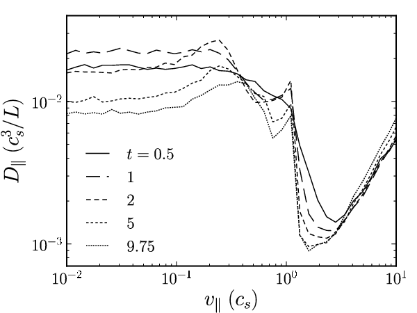
Figure 8 shows the time dependence of our test particle diffusion coefficients measured over different time baselines, for a simulation with $\dot{\epsilon}=0.01\,c_{s}^{3}/L$ and $v_{\perp}=c_{s}$. Perfectly overlying curves measured at different times would indicate perfectly diffusive behavior. We observe time dependence which is generally not perfectly diffusive, and is typically somewhat subdiffusive, in that e.g. $\langle(\delta v_{\parallel})^{2}\rangle$ scales somewhat less than linearly with $t$.

For smaller turbulence amplitudes, one might in principle expect the velocity diffusion coefficient to approach the sharp resonance of quasilinear theory, because the turbulence becomes increasingly weak on the outer scale. For example, in the simulation plotted in Figure 8, the amplitude of the turbulence is such that the turbulence is weak on the outer scale, with $v_{L}\simeq 0.16\,c_{s}\ll v_{A}$. Our model of a weak turbulence cascade in Appendix B predicts a rather sharp resonance, for these parameters. However, no obvious resonance is present in the test particle results shown in Figure 8.

We believe that this is the result of phase-decorrelation broadening, as discussed in §III.2.4. This decorrelation effect acts in addition to the primary wave-decay decorrelation model discussed in this paper. In turbulence, as discussed in §III.2.4, there is a typical wave-particle phase decorrelation time given by $t_{\mathrm{ph}}^{-1}\sim k_{\parallel}^{2/3}D_{\parallel}^{1/3}$ (if the particle velocity change is diffusive) or $t_{\mathrm{ph}}^{-1}\sim k_{\parallel}v_{\perp}M_{A}^{1/2}$ (if ballistic), and we can use this to predict a broadening width $\Delta v_{\parallel}$ by equating the linear frequency with the decorrelation frequency, as in §VI.2.

For the diffusive phase-decorrelation broadening, $\Delta v_{\parallel}\sim(D_{\parallel}/k_{\parallel})^{1/3}$. For the results in Figure 8, this approach predicts $\Delta v_{\parallel}\sim 0.09\,c_{s}$, evaluated at $k_{\parallel}=4\pi/L$. This is well less than the measured broadening. On the other hand, the ballistic (bounce-time) phase-decorrelation broadening gives $\Delta v_{\parallel}\sim v_{\perp}M_{A}^{1/2}\sim 0.34\,c_{s}$, which is consistent with the measured broadening to within a factor of $\sim\!2$. We also note that the double-peaked features in $D_{\parallel}$ in Figure 8 are similar to those plotted in Appendix A, where we consider the interaction of test particles with one ideal wave.

In order to make a quantitative comparison between our analytical heating rates and our test particle calculations, we will use the explicitly parameterized diffusion coefficients of Equations 10, 13, and 19, corresponding respectively to our exponential-decorrelated TTD, Gaussian-decorrelated TTD, and FTB models. Throughout this section, we will generally assume all species are at a constant reference temperature of $kT=\,m_{s}v_{s}^{2}$. Thus the important scaling is with respect to $v_{s}$ (or $m_{s}$, equivalently). We choose $\gamma=1$ and $\gamma=0.5$ for the exponential and Gaussian decorrelation models, respectively, as these values provide a reasonable fit to our simulations.

We simulate distributions of particles that are Maxwellian in $v=(v_{\perp}^{2}+v_{\parallel}^{2})^{1/2}$, and calculate their heating rate $\dot{E}\equiv(E_{f}-E_{i})/(t_{f}-t_{i})$. We normalize the initial energy density of the distribution to $3/4\,\rho c_{s}^{2}$, so that the test particles represent the energy of the ions or electrons in a proton-electron isothermal MHD fluid. (Because we use test particles, all of our heating rates may be straightforwardly adapted to a different particle density by multiplying by a factor $\rho_{\mathrm{test}}/\rho$.) We calculate a numerical heating rate by fitting a straight line to the test particle energy as a function of time, from $t=0.25-1\,L/c_{s}$.

We then determine the coefficients $\{C_{1},C_{2},C_{3},C_{4}\}$ in the analytic models for $D_{\parallel}$ by comparison to the test particle diffusion coefficients. For each value of $\dot{\epsilon}$, we focus on the value of $v_{\perp}$ where our Gaussian analytic model best matches the location of the high-$v_{\parallel}$ cutoff in the parallel diffusion coefficient (in e.g. Figure 7, this cutoff is around $v_{\parallel}\sim 2\,c_{s}$). Then we choose the $C_{i}$ to match the normalization. The normalization of the analytic curve in Figure 7 is a result of this procedure.

Finally, we calculate the associated “analytic heating rates” by numerically evaluating the integral in Equation 20 (integrating the diffusion equation over parallel and perpendicular velocities) using our fits for the dimensionless coefficients $C_{i}$. We expect the $C_{i}$ to depend only weakly on parameters of the turbulence such as $\dot{\epsilon}$, $L$, etc. In Table 2, we provide our approximate values for these normalization coefficients for three runs at $\dot{\epsilon}=$ 0.01, 0.1, and $1\,c_{s}^{3}/L$, all at $\beta=1$; we discuss the dependence on $\beta$ in §VI.5. Over a factor of 100 in $\dot{\epsilon}$, the $C_{i}$ do not change significantly.

Figure 9 shows how the analytic heating rates compare to our test particle results for several different values of $\dot{\epsilon}$. Our numerically calculated heating rates never asymptote to a constant at high-$v_{s}$. It is thus clear that the Gaussian decorrelation function (orange curves) provides a better fit to the simulation data (black curves) in the high-$v_{s}$ regime, where it scales as $\ln{(v_{s})}/v_{s}$, as opposed to the exponential decorrelation prescription (blue curves), which is independent of $v_{s}$. Similarly, the delta function heating rate (pink curves) are typically too steep. In the high velocity regime, the heating rates are reasonably well-fit by a functional form $\dot{\epsilon}_{\mathrm{part}}\simeq 0.33\,v_{L}^{2}(v_{s}/c_{s})^{-0.4}$, though this expression only applies for $\beta=1$.

The dominant heating mechanism in Figure 9 depends on the thermal velocity of the test particles. Above the linear theory resonance at $v_{\parallel}\sim v_{\mathrm{slow}}$, the TTD contribution to the diffusion coefficient scales like $\mu^{2}/v_{\parallel}^{\alpha}\propto v_{\perp}^{4}/v_{\parallel}^{\alpha}$, where $\alpha=$ 2 or 3 depending on the decorrelation model. Thus, in the bulk of an isotropic thermal distribution, where $v_{\perp}\sim v_{\parallel}\sim v_{s}$, TTD is increasingly important at higher $v_{s}$. For low thermal velocity particles, on the other hand, $\mu\rightarrow 0$ and FTB dominates.

As discussed in §IV, linear theory implies an asymptotic heating rate $\dot{E}\propto v_{s}^{-1}$ for high $v_{s}$. This in turn implies that electrons, with thermal velocity $v_{e}=\sqrt{m_{p}/m_{e}}\,v_{p}\simeq 43\,v_{p}$ (where $m_{p}$ and $v_{p}$ are respectively the mass and thermal velocity of protons) are heated much less effectively than protons by the compressive fluctuations in $\beta\sim 1$ MHD turbulence. In Table 3, we provide estimates of $\dot{E}_{p}/(\dot{E}_{p}+\dot{E}_{e})$, the proton-to-total heating ratios in our test particle simulations, for a range of $\dot{\epsilon}$ and $\beta$. We assign protons a value of $v_{s}=c_{s}/\sqrt{2}$, appropriate for an equal-temperature electron-proton plasma. These calculations indicate that the electron heating rate is typically smaller than the proton heating rate by a factor of 2-5, rather than 43. This is primarily due to the asymptotic $\ln{(v_{s})}/v_{s}$ scaling of the simulated heating rates, corresponding to our Gaussian decorrelation model (see eqn. 25). It is interesting to note that the proton-to-total heating rates we find are consistent with empirical inferences of proton vs. electron heating in the solar wind [14], both in magnitude and in the increasing electron heating for smaller $\beta$.

In Figure 9, our analytic calculations with Gaussian resonance broadening overestimate the magnitude of the TTD heating at high $v_{s}$, particularly for smaller $\dot{\epsilon}$. This is for two reasons. The first is that we fit heating rates over the baseline $t=[0.25,1]\,L/c_{s}$. However, because the distributions are driven away from isotropy, the heating rate becomes less efficient over time, and so the test particle energy increases somewhat sub-linearly. Our analytics assume instead an isotropic Maxwellian at the original thermal velocity.

A more important effect is that the analytic model used in Figure 9 is purely strong turbulence, with $\omega_{\mathrm{nl}}\sim\omega_{\mathrm{linear}}$ (see §III.2.1). However, the turbulence in the simulations with lower $\dot{\epsilon}$ is in fact weaker, with $\omega_{\mathrm{nl}}<\omega_{\mathrm{linear}}$. We consider the diffusion coefficients resulting from a combination of weak and strong turbulence in Appendix B; this results in a sharper resonance which approaches the delta-function of linear theory in the $M_{A}\rightarrow 0$ limit. Thus we might expect a heating rate closer to the linear theory heating rate (the pink curves in Figure 9) for the runs with smaller $\dot{\epsilon}$, as indeed is the case in Figure 9. However, this interpretation is complicated by the fact that we do not find a clear peak in the test particle velocity diffusion coefficients at low $\dot{\epsilon}$ (see Figure 8). This is likely due to phase-decorrelation broadening, as discussed in §III.2.4.

Figure 10 shows the simulated heating rates for a thermal distribution of particles for several different values of plasma $\beta$ at fixed $\dot{\epsilon}=0.1\,c_{s}^{3}/L$, measured over a longer baseline of $t=[1,5]\,L/c_{s}$. We do not attempt to make a quantitative comparison with our analytic model. However, qualitatively, three effects are clear. First, FTB heating at low $v_{s}$ decreases in effectiveness at low $\beta$. This is due to the decreasing curvature of the typical magnetic field line involved in FTB interactions: $v_{L}/v_{A}$ decreases as $\beta$ decreases at fixed sound speed and $\dot{\epsilon}$.

Second, the contribution of slow modes to TTD decreases with decreasing beta. The fraction of the slow mode energy in parallel magnetic field compressions is $\propto\beta/(\beta+1)$. Thus, at low $\beta$ TTD heating due to the slow modes becomes less important.

Finally, for $\beta=0.1$, there is a clear bump in the heating rate at high thermal velocities, which moves to lower $v_{s}$ at higher $\beta$. We associate this peak with TTD heating by fast modes, which have a phase velocity approaching $v_{A}$ in the low-$\beta$ limit. The reduced heating in the $\beta=0.1$ case relative to the $\beta=0.3$ is simply due to the fact that our simulations have a greatly reduced proportion of fast mode energy at lower $\beta$, by a factor of $\sim\!3$.

Figure 11 shows the heating rate of a thermal distribution for different $t_{\mathrm{corr}}$, the correlation time of the Ornstein-Uhlenbeck process with which we drive the turbulence. Over a factor of $\sim\!400$ in $t_{\mathrm{corr}}$, there is only a factor of $\sim\!4$ change in the heating rate; this suggests that to zeroth order, our results are insensitive to the value of $t_{\mathrm{corr}}$. However, when $t_{\mathrm{corr}}\rightarrow t_{\mathrm{MHD}}$ (not shown in Fig. 11), where $t_{\mathrm{MHD}}$ is the MHD timestep, we find that our results approach the limit of an uncorrelated driving scheme (typically, $t_{\mathrm{MHD}}\sim 8\times 10^{-4}\,L/c_{s}$ in our highest resolution simulations). In this limit, we find acceleration mimicking the cyclotron resonance for high-gyrofrequency particles which should not be resonant, because of the artificially high frequencies introduced by the driving [42, see also].

Increasing $t_{\mathrm{corr}}$ from this minimum value while fixing other properties of the turbulence systematically affects the turbulent kinetic energy in each of the MHD modes. The other physically relevant timescale in our calculations is the outer-scale eddy turnover time, which for our fiducial simulation (see Table 1) is approximately $t_{\mathrm{eddy}}\sim L/v_{L}$, which is approximately given by $\sim 3\,L/c_{s}$ for the fiducial case. Again applying the Fourier spectral decomposition of [13], increasing $t_{\mathrm{corr}}$ from 0.01 $L/c_{s}$ to 4.0 $L/c_{s}$ decreases the Alfvénic energy from 55% to 45%, decreases the fast mode energy from 15% to 3%, and increases the slow mode energy from 30% to 45% (while decreasing the overall kinetic energy in the turbulence by roughly 30%). Note that we hold the input power $\dot{\epsilon}$ fixed as $t_{\mathrm{corr}}$ varies.

We also find that despite driving no modes with parallel wavelengths longer than $L/2$, long-wavelength modes with $k_{\parallel}v_{A}\sim t_{\mathrm{corr}}^{-1}$ naturally appear in the developed turbulence. We believe that this is due to frequency-matching between the correlation time of the driving and the natural frequency of long-parallel-wavelength modes (see Appendix C).

These varying proportions of energy affect the thermal heating rate in ways which are largely consistent with our interpretation of the heating (see Fig. 11). The decreasing energy in fast modes manifests itself in a factor of $\sim\!4$ decrease in the TTD heating rate at high thermal velocity, while the increase in slow mode energy contributes to increasing the heating rate just below $v_{s}\sim c_{s}$. The decrease in FTB heating is consistent with the decrease of $v_{L}$ at longer correlation times.

In previous sections, we have focused on short-timescale interactions between particles and turbulence to calculate diffusion coefficients and corresponding heating rates. On longer timescales, it is unclear whether these interactions produce a thermal or non-thermal evolution of the distribution function. To investigate this question, we carried out test particle simulations lasting for longer times.

Figure 12 shows the distribution function (dotted curve) resulting from a simulation with $\dot{\epsilon}=0.1\,c_{s}^{3}/L$ run for $t=20\,L/c_{s}$, corresponding to several eddy turnover times. The thermal energy of the particles has increased by $\sim\!50\%$. For comparison, Figure 12 also shows a Maxwellian with the same energy as the final distribution (long dashed curve). The final distribution is clearly non-thermal, in that there is somewhat more energy in high-velocity particles, and less for low-velocity particles. However, the distribution is only weakly non-thermal, in that there is no evidence for the formation of a power-law tail at high velocities.

This weak non-thermality is not that surprising, as even our broadened TTD resonance diffusion coefficient is largest for particles with $v_{\parallel}\sim v_{A}$. Our result is inconsistent with recent work claiming that compressible turbulence generically leads to non-thermal power law tails $f(v)\propto v^{-5}$, as observed in the solar wind [23, 24, see]. However, their formalism assumes an isotropic or nearly isotropic distribution function, enforced by particle collisions or microscale instabilities, and has been criticized by [38] and [53], among others. We will investigate this point in more detail in future work.

References

- [1] Bartosch, L. 2001, International Journal Of Modern Physics, 12, 851
- [2] Beresnyak, A. 2011, Physical Review Letters, 106, 18
- [3] —. 2012, Monthly Notices of the Royal Astronomical Society, 422, 3495
- [4] Bieber, J. W., Matthaeus, W. H., Smith, C. W., Wanner, W., Kallenrode, M.-B., & Wibberenz, G. 1994, The Astrophysical Journal, 420, 294
- [5] Boldyrev, S. 2006, Physical Review Letters, 96, 1
- [6] Boris, J. 1970, in Proceedings of the Fourth Conference on Numerical Simulations of Plasmas, Naval Research Lab, 3–67
- [7] Chandran, B. D. G. 2000, Physical Review Letters, 85, 4656
- [8] —. 2003, The Astrophysical Journal, 599, 1426
- [9] Chandran, B. D. G., Li, B., Rogers, B., Quataert, E., & Germaschewski, K. 2010, The Astrophysical Journal, 720, 503
- [10] Chaston, C. C. 2004, Journal of Geophysical Research, 109, 1
- [11] Chen, C. H. K., Mallet, A., Yousef, T. A., Schekochihin, A. A., & Horbury, T. S. 2011, Monthly Notices of the Royal Astronomical Society, 415, 3219
- [12] Cho, J., & Lazarian, A. 2002, Physical Review Letters, 88, 1
- [13] —. 2003, Monthly Notices of the Royal Astronomical Society, 345, 325
- [14] Cranmer, S. R., Matthaeus, W. H., Breech, B. A., & Kasper, J. C. 2009, The Astrophysical Journal, 702, 1604
- [15] Cranmer, S. R., & van Ballegooijen, A. A. 2003, The Astrophysical Journal, 594, 573
- [16] —. 2012, The Astrophysical Journal, 754, 92
- [17] Cranmer, S. R., van Ballegooijen, A. A., & Edgar, R. 2007, The Astrophysical Journal Supplement Series, 171, 520
- [18] Dmitruk, P., Matthaeus, W. H., & Seenu, N. 2004, The Astrophysical Journal, 617, 667
- [19] Drake, J. F., Cassak, P. A., Shay, M. A., Swisdak, M., & Quataert, E. 2009, The Astrophysical Journal, 700, L16
- [20] Drake, J. F., Swisdak, M., Che, H., & Shay, M. A. 2006, Nature, 443, 553
- [21] Dupree, T. 1966, Physics of Fluids, 9, 1773
- [22] Fermi, E. 1949, Physical Review, 75, 1169
- [23] Fisk, L., & Gloeckler, G. 2007, Proceedings of the National Academy of Sciences of the United States of America, 104, 5749
- [24] —. 2008, The Astrophysical Journal, 686, 1466
- [25] Galtier, S., Nazarenko, S. V., Newell, A. C., & Pouquet, A. 2000, Journal of Plasma Physics, 63, 447
- [26] Gary, S. P., & Borovsky, J. E. 2008, Journal of Geophysical Research, 113, 1
- [27] Goldreich, P., & Sridhar, S. 1995, The Astrophysical Journal, 438, 763
- [28] —. 1997, The Astrophysical Journal, 485, 680
- [29] Grappin, R., & Müller, W.-C. 2010, Physical Review E, 82, 2
- [30] Hazeltine, R., & Waelbroeck, F. 1998, The Framework of Plasma Physics (Perseus Books)
- [31] Higdon, J. C. 1984, The Astrophysical Journal, 285, 109
- [32] Hockney, R., & Eastwood, J. 1981, Computer Simulation Using Particles (CRC Press)
- [33] Howes, G. G., Bale, S. D., Klein, K. G., Chen, C. H. K., Salem, C. S., & TenBarge, J. M. 2011a, 4
- [34] Howes, G. G., Cowley, S. C., Dorland, W., Hammett, G. W., Quataert, E., & Schekochihin, A. A. 2008, Journal of Geophysical Research, 113, 1
- [35] Howes, G. G., TenBarge, J. M., & Dorland, W. 2011b, Physics of Plasmas, 18, 102305
- [36] Jiang, Y. W., Liu, S., & Petrosian, V. 2009, The Astrophysical Journal, 698, 163
- [37] Jokipii, J. R. 1966, The Astrophysical Journal, 146, 480
- [38] Jokipii, J. R., & Lee, M. A. 2010, The Astrophysical Journal, 713, 475
- [39] Kennel, C., & Engelmann, F. 1966, Physics of Fluids, 9, 2377
- [40] Kraichnan, R. H. 1965, Physics of Fluids, 8, 1385
- [41] Leamon, R. J., Smith, C. W., Ness, N. F., & Wong, H. K. 1999, Journal of Geophysical Research, 104, 22331
- [42] Lehe, R., Parrish, I. J., & Quataert, E. 2009, The Astrophysical Journal, 707, 404
- [43] Lemaster, M., & Stone, J. 2009, The Astrophysical Journal, 691, 1092
- [44] Lithwick, Y., & Goldreich, P. 2001, The Astrophysical Journal, 562, 279
- [45] Maron, J. L., & Goldreich, P. 2001, The Astrophysical Journal, 554, 1175
- [46] McChesney, J., Stern, R., & Bellan, P. 1987, Physical Review Letters, 59, 1436
- [47] Montgomery, D., & Turner, L. 1981, Physics of Fluids, 24, 825
- [48] Ng, C. S., & Bhattacharjee, A. 1997, Physics of Plasmas, 4, 605
- [49] Perez, J. C., & Boldyrev, S. 2008, The Astrophysical Journal, 672, L61
- [50] Qin, G., Matthaeus, W. H., & Bieber, J. W. 2006, The Astrophysical Journal, 640, L103
- [51] Quataert, E. 1998, The Astrophysical Journal, 20, 978
- [52] Quataert, E., & Gruzinov, A. 1999, The Astrophysical Journal, 520, 248
- [53] Schwadron, N. A., Dayeh, M. A., Desai, M., Fahr, H., Jokipii, J. R., & Lee, M. A. 2010, The Astrophysical Journal, 713, 1386
- [54] Shalchi, A., Bieber, J. W., Matthaeus, W. H., & Qin, G. 2004, The Astrophysical Journal, 616, 617
- [55] Shalchi, A., & Schlickeiser, R. 2004, Astronomy & Astrophysics, 420, 799
- [56] Shebalin, J. V., Matthaeus, W. H., & Montgomery, D. 1983, Journal of Plasma Physics, 29, 525
- [57] Stix, T. 1992, Waves in Plasmas (Springer)
- [58] Stone, J., Gardiner, T. A., Teuben, P., Hawley, J. F., & Simon, J. B. 2008, The Astrophysical Journal Supplement Series, 178, 137
- [59] Verdini, A., & Grappin, R. 2012, Transition from weak to strong cascade in MHD turbulence
- [60] Weinstock, J. 1969, Physics of Fluids, 12, 1045
- [61] Yan, H., & Lazarian, A. 2004, The Astrophysical Journal, 614, 757
- [62] —. 2008, The Astrophysical Journal, 673, 942
Appendix A Landau-type Resonance Between Test Particles and One Wave
To consider the effects of particle trapping and bin-crossing on our method for measuring velocity diffusion coefficients, we have simulated a simpler self-contained one-dimensional toy problem, where particles feel a sinusoidal, travelling acceleration of the form . This is effectively the Landau problem with test particles. (The toy problem is independent of Athena, but we have confirmed that the results are qualitatively identical to test particles interacting with a single slow mode wave in Athena.)
The mean-square change in the velocity of test particles for several waves with different amplitudes is shown in Figure 13. We plot because this quantity converges to a constant at long times. If each bin in were truly a delta-function, and there was no numerical loss of accuracy, then for test particles in a given bin would reach a maximum after approximately (corresponding to half of the wave-particle interaction time), and then decrease back to zero as every particle returned to its original phase with respect to the wave, though offset by . However, because particles are smoothly distributed in velocity within each bin, slight initial velocity differences lead to the destruction of this phase coherence over time, and converges to a constant value of roughly half its maximum.
Acceleration by a small-amplitude wave produces a very sharp resonance around the wave phase velocity, while particle trapping significantly broadens the resonance for large-amplitude waves. For this problem, a small amplitude wave is one for which , where is the linear wave period and is the time for a particle’s velocity to change significantly due to the wave-particle interaction. The transport in velocity space is not truly diffusive for this toy problem, except for particles very near the resonance.
The results of this simple problem are directly analogous to test particles interacting with MHD turbulence. When (where is the time required for particles to significantly move out of phase with a wave), particles experience significant acceleration and quickly fall out of phase with a previously resonant wave, leading to strong resonance broadening. The situation in turbulence is discussed in §III.2.4.
Appendix B Resonance Broadening in Weak Turbulence
B.1. Turbulence Model
In the main text, we considered a resonance broadening model where the underlying turbulence spectrum was purely strong GS turbulence. In this appendix, we discuss an expansion of the model to the case of weak turbulence.
We consider MHD turbulence that is driven isotropically with an outer scale eddy velocity . The turbulence at the outer scale is weak in the sense that the linear time scale for wave propagation is shorter than the nonlinear time scale for eddy turnover, , where isotropy implies that . This implies that waves live for more than one wave period before they decay. We may express this weak turbulence requirement more generally by noting that the non-linearity parameter , where and refer to scales smaller than , and is the turbulent eddy velocity on that scale.
However, weak turbulence cascades only in the perpendicular direction to higher [56, 25], while no structure on smaller parallel scales develops. This implies a 1D power spectrum [48]. However, , so that the non-linearity increases at smaller scales. Eventually, when , the turbulence reaches the strong critically balanced state of GS, and the cascade proceeds to smaller scales at fixed of order unity. Critical balance refers to the balance of wave and eddy time scales. This implies that most of the turbulent energy is contained in eddies with , and a 1D power spectrum . The transition between the weak and strong regimes occurs at a wavenumber , where is the Alfvénic Mach number at the outer scale.
More quantitatively, we define the 3D power spectrum as