Field induced stationary state for an accelerated tracer in a bath
Abstract
Our interest goes to the behavior of a tracer particle, accelerated by a constant and uniform external field, when the energy injected by the field is redistributed through collision to a bath of unaccelerated particles. A non equilibrium steady state is thereby reached. Solutions of a generalized Boltzmann-Lorentz equation are analyzed analytically, in a versatile framework that embeds the majority of tracer-bath interactions discussed in the literature. These results –mostly derived for a one dimensional system– are successfully confronted to those of three independent numerical simulation methods: a direct iterative solution, Gillespie algorithm, and the Direct Simulation Monte Carlo technique. We work out the diffusion properties as well as the velocity tails: large , and either large , or in the vicinity of its lower cutoff whenever the velocity distribution is bounded from below. Particular emphasis is put on the cold bath limit, with scatterers at rest, which plays a special role in our model.
Keywords:
Boltzmann equation, Out-of-equilibrium, Stationary state, Distribution tailsI Introduction
The propagation of a single test particle (or ”tracer”) with mass accelerated by an external field in a stationary bath of particles with mass was first studied by Lorentz in 1905 [1] as a kinetic approach of conduction in a metal. In this model, an electric field accelerates non-interacting electrons, which diffuse among a random configuration of static obstacles - the atoms - acting as infinitely massive scatterers (), with a simple hard sphere electron-atom collision rule. Lorentz assumed the velocity distribution of the electrons to obey a Maxwell-Boltzmann law with a small correction, and was able to give an estimate of the conductivity of metals from microscopic parameters. It was later shown that this perturbed Maxwell-Boltzmann distribution cannot be a stationary solution of the problem [2]: the constant acceleration confers an ever-increasing amount of energy to the electron, which cannot be dissipated in the described collision process. Its velocity variance consequently diverges over time, while the mean velocity (and hence the current) stays finite and close to the Lorentz result on a certain time scale studied in [3, 4] then vanishes at long times. However, a stationary solution may exist if the tracer is allowed to transfer some energy to the surrounding medium, for instance when collisions are dissipative [5] or with a finite mass ratio .
The case was therefore subsequently considered [6], as an extension of Résibois’ field-less ”self-diffusion problem” [7], wherein one studies the diffusive properties of identical gas particles at equilibrium by following a single unaccelerated tracer. The bulk of ulterior developments on this modified Lorentz problem focused on asymptotic and relaxation properties [8, 9, 10, 11, 12, 13]. Recently, the model was used as a paradigm for the study of microscopic entropy production and fluctuation relations in non equilibrium systems [14, 15], and to discuss the force-velocity relation [16] as measured in experiments [17].
In what follows, we will mostly concentrate on the one dimensional version of the model, the several variants of which addressed in the literature differ first by the choice of different bath velocity statistics (at rest with [6], dichotomous [8, 10, 12] or Gaussian [9, 10, 13]) and second by the collision kernel accounting for grain interactions, that can be indexed by a continuous parameter (hard rods with in most earlier works, but also for Maxwellian rods [18] or the so-called ”very hard rods” having [13]). Moreover, in addition to mass ratio and field strength that play a key role, collisions between the tracer and bath particles can be inelastic [19, 20]. The ensuing parameter space is therefore large, with associated rich behavior. At the Boltzmann equation level, our goal is here to provide a comprehensive view of the tracer stationary velocity distribution function, that in all generality will be denoted : it depends on three parameters (, and a number that lumps mass ratio and dissipation in a single constant [11, 21]), and is furthermore a functional of bath velocity distribution . The reason for considering an arbitrary bath distribution lies in the wide spectrum of non-equilibrium steady states that can be achieved upon driving granular gases with different energy injection mechanisms [22, 20]; Stretched exponentials are often encountered here. A tracer in an evolving (e.g. freely cooling) bath may also be of interest [23], assuming that it can reach a state with no time dependence except through .
Before rationalizing the behavior of , the model will be detailed in section II, where a convenient integral form will be derived from the Boltzmann equation. This provides the basis for an efficient numerical resolution algorithm, that will be described in section II.3, together with the more versatile Gillespie and Direct Simulation Monte Carlo techniques. Thereby equipped with three different numerical schemes, we will put to the test in section III analytical results to be derived for the velocity tails and diffusive properties, for an arbitrary bath distribution. The cold bath setting will be put forward and solved in Section IV as a relevant model onto which more general situations can be mapped, while particular attention will be paid in Section V to the low velocity limit for bounded bath distributions. Finally, our conclusions will be presented in Section VI.
II The model, its integral reformulation, and numerical resolution
II.1 Statement of the problem
We consider the one dimensional motion of a single particle of mass , accelerated by a constant force through a bath. The bath is made up of unaccelerated particles of mass , having a stationary velocity distribution function with characteristic velocity . This velocity scale is used for the nondimensionalization of both the velocity of the tracer and the force where is the linear mass density in the bath, and being the corresponding variables with physical dimensions.
The time dependent tracer velocity distribution is indexed by a parameter that specifies the type of tracer-bath interactions, and is denoted . The dependence on other parameters and on is left implicit unless necessary.
The dynamics under study is governed by the linear Boltzmann (or Boltzmann-Lorentz) equation
| (1) |
Here, is the collision operator
| (2) |
where the post collisional velocity of a binary encounter can in general be written:
| (3) |
Such an expression unifies elastic and dissipative collision through the dimensionless parameter
| (4) |
being the restitution coefficient which describes the inelasticity of tracer-bath collisions (elastic if , and inelastic if [19]). It is remarkable that any system with dissipative collisions may therefore be mapped to an elastic system with a different mass ratio , leading to the same dynamics and stationary states for the tracer [21, 24]. The “memory-less” situation is of particular interest due to its simplicity: each collision with a bath particle erases any memory of the tracer’s previous state, and this case has been thoroughly studied and solved in different settings [6, 9, 21]. The original Lorentz model corresponds to , or in its inelastic variant [5], while the opposite Rayleigh limit (of an infinitely massive tracer) was considered in [10].
The exponent introduced in (2) encodes different scattering behaviors [20, 25]; The three most common models are corresponding to Hard Rods, for Maxwell particles and for Very Hard Rods, the latter two approaches being often invoked to reproduce qualitatively some hard rod properties while simplifying calculations [26]. Their merits are discussed in [10] among others, but it will be shown in later sections that the value of may affect significant properties of the solution, some of which may exhibit crossovers depending on the value of . Negative values of have been shown to produce some interesting phenomenology in the Lorentz model, such as the remarkable runaway effect [27], however our one-dimensional model with finite mass ratio produces well-behaved solutions if and we shall restrict our study to this case.
It should also be noted that the molecular chaos assumption underlying the Boltzmann equation approach –motivated by the desire to derive analytical results– prevents the occurrence of single-file diffusion [28]. However, when possible, we will discuss systems with a higher dimensionality, for which the molecular chaos assumption is justified in the low density limit.
It has been shown [13] that the velocity distribution quickly relaxes to a stationary solution , on which we shall concentrate in the remainder: it obeys
| (5) |
which expresses the balance between the energy received from the external field , and the energy transfered to the bath through collisions. Eq. (5) may be rewritten as
| (6) |
where
| (7) |
The latter quantity is the velocity-dependent collision frequency in the gas, and is given by
| (8) |
which is the gain term of the collision operator, i.e. the transition rate toward velocity through the collision process, integrated over all possible initial velocities (dummy variable ). Clearly, is the equilibrium solution for vanishing acceleration, when detailed balance entails that entering and leaving fluxes are equal at each point in phase space. In this field-free case (), two situations discussed in [21] ensure that the tracer velocity distribution is directly given by the bath distribution: first, for memory-less collisions (), we have
| (9) |
for arbitrary bath statistics, as can be checked from (8). Second, when the bath distribution is Gaussian , one finds (see also [11])
| (10) |
In general however, the tracer distribution differs from the bath distribution even in this unaccelerated limit, except in the tails (see section III).
We will later need to consider the distribution of pre-collisional velocities, i.e. velocities sampled right before each collision rather than uniformly over time. This distribution is usually biased toward high velocities –which have enhanced collision rate as long as – and it is given by [29]
| (11) |
where the mean collision frequency is defined as
| (12) |
II.2 Implicit form
It proves convenient to recast the stationary probability density function as an implicit integral form. To this end, we write the velocity of the tracer at any given time as , with the velocity that was acquired during its last encounter with a scatterer, and the contribution of the driving field during the timespan of ballistic flight . We next consider the conditional probability that no collision occurs during for a tracer starting with velocity , which involves the velocity-dependent collision frequency :
| (13) |
We then need the probability density for the post-collisional velocity . By definition it is proportional to the gain term of the Boltzmann operator, which covers all collision events from which the tracer may emerge with velocity (proper normalization of the probability densities will be enforced a posteriori). Finally, integrating over all possible time-spans , the stationary tracer velocity distribution can be written
| (14) |
It can be checked by direct calculation that the above function obeys the Boltzmann-Lorentz equation (6). A similar equation may be found for the time-dependent solution, with explicit dependence in the initial condition :
| (15) |
where is defined as in (8) substituting for . This expression is useful for studying the relaxation process toward the stationary solution in the limit [13]. The stationary solution may also be interpreted as an eigenfunction of a linear integral operator , associated with the eigenvalue :
| (16) |
where the kernel is identified from equation (14):
| (17) |
with
| (18) |
This form simplifies in the case of Maxwell particles ()
| (19) |
The kernel then reduces to a Laplace transform
| (20) |
If furthermore , the solution itself becomes a transform of the bath distribution (as noted in [10, 13] in the special case of a Gaussian bath ):
| (21) |
For general values of and however, no obvious simplification can be found for the kernel . Expression (16) nevertheless allows for efficient numerical solving, as we now describe.
II.3 Numerical resolution of the Boltzmann-Lorentz equation
Three different techniques have been employed to obtain numerically the tracer velocity statistics. We start by summarizing their main features, before testing their compatibility.
II.3.1 Numerical integration and iterative solving
The operator derives from the Boltzmann-Lorentz equation, which by construction preserves the total probability in phase space. must therefore conserve the integral of any function upon which it is applied. This implies that its spectrum is reduced to two eigenspaces, associated with eigenvalues (where the sought solution lies) and (with non-physical eigenfunctions having vanishing integral). The application of therefore acts as a projection on the eigenspace associated with the eigenvalue .
Numerically, discretizing into a matrix and starting with a random vector, the iterative application of and subsequent normalization of the vector should converge toward the physical solution. Indeed all elements of are positive, therefore its largest eigenvalue is non-degenerate by the Perron-Frobenius theorem, associated with a positive eigenvector. This unique eigenvector coincides with the physical solution obtained through numerical simulations or determined analytically whenever possible, and this technique allows for fast computation of the solution to any precision, especially in the large velocity tails where other methods may become inefficient. At this point, we have to choose between two strategies: solving the eigenproblem numerically for the matrix , or alternatively applying the matrix iteratively until proper convergence is achieved. We have checked that both routes are equally precise and efficient, for a similar computational cost.
II.3.2 Gillespie algorithm
The second numerical technique used relies on the Gillespie algorithm, adapted to the Boltzmann-Lorentz equation by Talbot and Viot [30]. The salient features are as follows. We recall from (13) the conditional probability that no collision occurs during time for a tracer starting with the post-collisional velocity
| (22) |
This relationship may be inverted (either analytically or numerically by dichotomy, the latter being necessary for or with a non-Gaussian bath) to obtain , allowing us to randomly generate collisions times for the tracer, after having drawn uniformly in [0,1].
The velocity of the collision partner must then be generated with the correct weight . First, the flux of collisions is divided in two contributions, coming from the right and left of the tracer:
| (23) |
| (24) |
The probability of a collision coming from the right (resp. the left) is given by (resp. ). The direction of the next collision is thus determined using another random uniform number over . Depending on which side is chosen, given by
| (25) |
The velocity must be drawn with this weight, which is performed using an acceptance-rejection process: is generated according to the bath distribution (which significantly improves the efficiency in generating high velocities over a uniform generation with a cut-off), and then accepted with a probability
| (26) |
with the velocity for which is maximal (which can be computed analytically for ).
II.3.3 Direct Simulation Monte Carlo
We also used Direct Simulation Monte Carlo (DSMC) [31] simulations as an alternative to the Gillespie algorithm, in order to experiment easily on various baths and collision laws, without performing the (bath-dependent) analytical computations which increase the efficiency of the Gillespie method. DSMC differs from the previous approach in that instead of generating the correct collision times directly, a collision partner is drawn at each step for the tracer, with a velocity distributed according to the bath probability density function . This collision event is then accepted with probability
| (27) |
with and the maximal value encountered for at this point. The time counter is incremented by at each step. This procedure converges in a few hundred steps per particle toward a satisfactory evaluation of the correct collision frequency, as the observed velocity distribution for the tracer (over many realizations, and/or sampled uniformly over time) is then identical to the result of the Gillespie algorithm, or analytical computations whenever they can be performed.
This method is not significantly less efficient than the Gillespie algorithm, despite its lesser specificity. It can be extended to represent collisions in higher dimensionality –as required for the discussion in section III.2– by drawing a vector uniformly on the unit sphere and redefining
| (28) |
with the cross-section of the tracer-bath collisions. The post collisional velocity for the tracer is then given by
| (29) |
II.3.4 Assessing the three numerical techniques
The implicit route allows for efficient computation of the stationary tracer velocity distribution with important precision. Hereafter, it will be the method used whenever a specific prediction requires unusual numerical precision (good sampling of the tails). This will in particular be the case of Figs. 5 and 6. Among the three techniques, DSMC appears on the other hand to be the more versatile, since a change in the model parameter like softness exponent does not lead to any complication. Finally, Gillespie and DSMC algorithms are well suited to study the transient regime before the steady state is reached (see e.g. [10, 12, 13]), together with diffusive properties. Fig. 1 demonstrates the validity and consistency of all three techniques in two settings.

III Velocity tails and diffusive behavior
III.1 Asymptotics
As we shall disregard the time evolution of the system, the term ”asymptotic behavior” refers here to the behavior of the stationary tracer distribution for extreme values of the velocity. Rewriting the implicit equation (14) as
| (30) |
with and defined in (8) and (18), and assuming that both and decay exponentially we may use Laplace’s method to approximate the integral over . It is easily seen that
| (31) |
while we may choose a general stretched exponential expression for the tails of the bath distribution
| (32) |
where , as found in various granular systems [22, 32, 20]. Power-law tails are obtained in the limit , while corresponds to a uniform distribution with bounded support . We shall restrict ourselves to as becomes logarithmic when and we cannot expect an exponential decay of the integrand and apply Laplace’s method anymore.
We may gain intuitive insight into the large asymptotics by noting that competing effects are at work: such velocities may be reached either through collision with sufficiently energetic bath particles, or through acceleration without collision for a sufficiently long time. The relative importance of these effects is thus determined on the one hand by the abundance of energetic particles in the bath, characterized by the parameter , and on the other hand by the velocity-dependent collision frequency characterized by . Consequently, if is large enough compared to , the increase in collision frequency for high velocities is so steep that ballistic flight is interrupted before the tracer can be significantly accelerated. The largest velocities are therefore reached through collisions with energetic scatterers, and the Boltzmann equation is dominated by the gain term, entailing that the tracer distribution is pushed back toward the bath distribution. This may be seen as thermalization with the bath tails. If on the other hand is sufficiently large compared to , the bath tails are relatively depleted, while ballistic flight and acceleration are less impeded by the collision process. This corresponds to a prevalence of the loss term in the master equation: it is more probable for the tracer to have a large velocity before a collision (due to acceleration) than after it.
A more refined asymptotic analysis confirms the above qualitative features. Since the argument of the exponential in (30) decreases as , either the global maximum is located on the boundary at , or it corresponds to some local extremum such that the derivative of the argument vanishes
| (33) |
If the dependence of the integral receives no contribution from the term –the gain term of the Boltzmann equation is negated– and we have . This is possible only in the positive tail : when , all the local extrema eventually exit the interval and the global maximum is necessarily located at the boundary , regardless of the parameters and .
In the latter situation (for either tail), disappears from (30) –the loss term is negated– and we have
| (34) |
We search for self-consistent solutions using Laplace’s method, and find
| (35) |
as in the unaccelerated problem, where the dilation coefficient satisfies
| (36) |
For a Gaussian bath (for which ) it becomes which equals when collisions are elastic, as expected from thermalization.
The other solution to (34) is , provided that vanishes faster than so that the stationary point is asymptotically close to . This solution is self-consistent only if , as it then relates one tail to the other rather than equating the same tail in two different points.
Combining these observations, it appears that the leading behavior for is simply controlled by the value of the integrand of (30) at each of the two locations and , and switches from field-driven (due to the loss term) if the first dominates to thermalized if it is the second (see Table 1). For , however, the default behavior is thermalized, unless and the positive tail is field-driven. In that case, collisions may revert large velocities, and the left tail becomes the image of the right tail with .
|
![[Uncaptioned image]](1203.6759v3/phase_space.png)
| ||||||||||||||||||||||||||||||||
The large velocity scenario sketched in Table 1 is as follows. If , we recover the bath behavior in , in agreement with the intuitive argument outlined above, while if , the positive velocity tail exhibits a decay, hereafter referred to as the cold bath behavior. These expectations, disregarding subleading terms such as polynomial prefactors, are fully corroborated by Fig. 2.
If , both behaviors correspond to the same exponent, and prevalence of one process over the other depends on the value of the driving field compared to . For a Gaussian bath with , the borderline case corresponds to the hard-rod model, as depicted in the middle picture of Fig. 2: upon increasing the acceleration, the positive tail switches continuously from the field-independent expression when to the field-dependent when . The critical field, , reduces to unity in the memoryless case .
If , the onset of the positive tail behavior described above is given by the point where
| (37) |
Assuming this threshold is larger than the typical bath velocity (set to unity), there is an intermediate asymptotic range dominated by acceleration. The bath-like tail is thus expected to appear only when . If however , both the intermediate range and the (positive) tail are similarly field-driven, and no such clear-cut crossover can be observed.
Both cases are represented in Fig. 2 : the latter appears on the right-hand side, and the former on the left-hand side, where the crossover from the field-driven behavior to the bath-driven tail may be seen on the curve with (crosses). The intermediate asymptotics may nevertheless dominate over a large range of positive velocities, as can be seen for a higher value of (filled dots) where the thermalized tail has yet to appear.
In the strong-field limit , the threshold diverges and the field-driven behavior prevails for all over the whole parameter space of and . As can be seen from our choice of dimensionless variables in section II.1, this is equivalent to taking the limit of motionless bath particles while keeping constant : this limit is the so-called ”cold bath” that will be discussed in section IV and exhibits characteristic field-driven tails.
The opposite limit is singular as it suppresses this cold bath (field-driven) behavior altogether, rendering our discussion of limiting cases invalid as the only possible asymptotic behavior is the thermalized expression in both tails.

III.2 Diffusive properties
Another point of interest lies in the tracer diffusion coefficient , which was computed in [13] for a Gaussian bath and , using both its Green-Kubo expression and its definition in the hydrodynamic diffusion mode of the inhomogeneous Boltzmann-Lorentz equation. These two methods were shown to give identical results for and . The second method was also applied in [12] to the case and with a dichotomous bath, revealing the complex dependence of the diffusion coefficient on the magnitude of the field, with a minimum at finite , while this coefficient was shown to be monotonically increasing for and decreasing for in the aforementioned discussion of the Gaussian bath [13]. Here we consider an arbitrary bath distribution and parameter , and observe once again that the effects of acceleration and thermalization disentangle when . We also demonstrate that these results are qualitatively unchanged in higher dimensional space, as reported for other observables in [11].
As shown in the appendix, letting allows us to relate the diffusion coefficient to the variance of the tracer velocity through a simple combination
| (38) |
This variance may easily be determined recursively from that of the bath, by integration over the Boltzmann-Lorentz equation
| (39) |
with the th moment of the displaced bath distribution. Therefore, if the bath velocity distribution is centered and has finite variance,
| (40) |
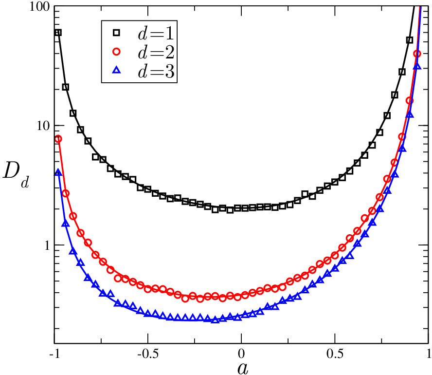
where is the mean velocity squared in the bath, chosen equal to in our dimensionless variables. This result is in agreement with [13] in the limit . It may be generalized to -dimensional space (see Appendix A)
| (41) |
where is the surface area of a -dimensional hypersphere. This prediction is in very good agreement with the DSMC simulation data shown in Fig. 3. In order to study the diffusive behavior of the tracer in these otherwise homogeneous simulations, its spatial coordinate is computed as the time-integral of the velocity. Between two collisions, the ”space counter” in the direction of the acceleration is thus incremented by with the velocity of the tracer during this free flight and the previously determined collision time.
IV The cold bath
In our previous discussion of the velocity tails for the tracer in a general bath, we have observed the prevalence of a ”cold bath” asymptotic behavior for certain values of the parameters, see Table 1. The cold bath refers to a particular limit of the general Lorentz problem, where the scatterers are motionless and their velocity distribution is represented by the Dirac delta function: it may be understood as the limit as discussed in III.1.
This setting has been studied for hard rods with [6] and in some limiting cases with [11]. Inserting in (7) gives and the Boltzmann-Lorentz equation takes the form of a functional-differential equation
| (42) |
which is reminiscent of relations found in other stochastic processes such as random walks and growth models on trees [33]. In the field-free case, this equation reverts to a class of random collision problems systematically studied by ben-Avraham et al. [34].
This system plays a prototypical role in the study of the general Lorentz problem for two reasons. First, it may be seen as the strong field limit () of any bath distribution as discussed in section III.1. Second, there are two exact mappings allowing to reduce a more general problem to the exactly solvable case of a Maxwellian tracer in a cold bath, with both and , if only either one of these conditions is verified. Indeed, given a cold bath distribution, we may derive the solution for any value of the collision kernel exponent from the Maxwellian solution . This may be seen if we define
| (43) |
which verifies
| (44) |
With the simple rescaling this equation is made to coincide with (42), which is associated to Maxwell particles.
On the other hand, for Maxwell particles () a theorem proved by Wannier [35] for the three-dimensional case and Eder and Posch [10] in one dimension gives the complete (time-dependent) solution for any bath distribution as a convolution over the cold bath solution
| (45) |
This relation holds as well for the stationary state which is under scrutiny here.
However Wannier’s convolution theorem does not hold for arbitrary values of , which prevents from extending this mapping to settings where both and are chosen different from the prototypical case (, ). Yet, this model still preserves many significant features of the general solution, as discussed previously.
IV.1 Explicit solution
The cold bath equation (42) may be rewritten as the implicit equation
| (46) |
where denotes the Heaviside function. This expression allows us to derive straightforwardly the solution for the ”memory-less” case
| (47) |
where it appears that the tracer velocity distribution has support on . The solution for any may be recovered from the aforementioned mapping, in order to study the dependence of quantities of interest, such as the mean velocity (note the choice of index to simplify this expression)
| (48) |
where is the Euler gamma function. Thus in agreement with the dimensional argument presented in [6]. It should be noted that, unless , this implies a breakdown of linear response: for , as discussed in [11].
We now derive the explicit solution for , considering Maxwellian particles (without loss of generality, as argued above) which verify
| (49) |
The general expression of the solution may be found by taking the Fourier transform of the function
| (50) |
which in turn verifies
| (51) |
| (52) |
Then by recurrence we may relate to . As , when . Furthermore due to the normalization of , hence
| (53) |
Taking the inverse transform (with some care as the position of the poles and the integration contour depend on the sign of both and )
| (54) |
From this expression, we may identify the asymptotic behavior for as the first non-zero term in the sum depending on the sign of and . We therefore obtain the characteristic ”cold bath” positive tail behavior presented in Table 1: when ,
| (55) |
The negative tail behavior however differs from the situations discussed in section III, where it was determined by the bath distribution. It is readily seen from (54) that negative velocities cannot be reached if : in that case, equation (3) entails that the tracer velocity is reduced but never reversed by collisions with bath particles. Once it has become positive due to acceleration, it may not become negative again, which ensures that the stationary solution has support on only. If however , the negative tail is given by
| (56) |
These asymptotic expressions for with are corroborated by numerical results in Fig. 4.
The moment hierarchy is obtained by a straightforward integration, and its general term is found
| (57) |
where using the -Pochhammer notation [36]
| (58) |
This symbol appears in combinatorics as a generalization of the Pochhammer symbol or rising factorial:
| (59) |
The expression converges in the limit to a standard function of known as the Euler function (not to be confused with the better known Euler totient function in number theory).
We may rewrite the cold bath solution (54), using the notation for the product over , and recognizing the exponential term as the solution for in (47) where the acceleration has undergone the rescaling . We obtain the concise formula
| (60) |
This structure is interesting in several respects: first, the sum converges very rapidly for the needs of numerical computation, and is found in excellent agreement with our simulation results. Second, due to the simple form of , using Wannier’s theorem to derive the full solution for Maxwell particles in any bath will only involve taking Laplace transforms of the bath distribution. An application to the Gaussian bath is given below. Finally, even though this structure will not be preserved for systems with arbitrary bath distribution and , it suggests that some significant traits of the general solution may be contained in the limiting case , which is more readily solved in any model, see e.g. [9, 13]. However, both analytical expressions (54) and (60) shed little light on the behavior of the cold bath solution for positive in the limit , which will warrant a separate investigation in section V.

IV.2 Application to the Gaussian bath
We now revisit some properties of one of the most extensively studied settings, the Maxwellian tracer in a Gaussian bath (, ) [9, 10, 13]. This will serve to demonstrate the application of results from the cold bath limit to arbitrary bath distributions, which we recall is exact for .
From Wannier’s convolution theorem we deduce that the solution in this setting is simply given by the Laplace transform of the Gaussian , as we previously saw in (21) (see also [13])
| (61) |
Inserting this expression in the series (60) allows for accurate numerical computation as well as asymptotic analysis for .
We thus recover a result that was obtained in Ref. [10], where use was made of a method specific to this choice of bath and collision kernel: using Mehler’s formula [37], it is possible to compute the analytical solution of the Boltzmann-Lorentz equation as an expansion in terms of the Hermite Polynomials
| (62) |
However, this expansion diverges for any value of the parameters, even at vanishing velocity as for even , while for odd . Consequently, the expansion must be put under a different form to allow for numerical computation. It is suggested in [10] that, owing to a theorem by Euler
| (63) |
from which, interchanging the sums, one finds as expected
| (64) |
Finally, we may be interested in seeing how exactly the hierarchy of moments with a Gaussian bath relates to its cold bath equivalent. We compute the moment-generatrix, using the connection between the Hermite polynomials and the derivatives of the Gaussian
| (65) |
with
| (66) |
from which we derive a general expression for the -th moment of :
| (67) | |||||
The term (which is the leading order for large ) is recognized as the corresponding moment in the cold bath (57), while the following terms appear to be specific to the Gaussian setting.
V Non-negative stationary distribution
The solution for exhibits some peculiar properties in the cold bath configuration: the tracer velocity can be reduced but never reversed by a collision. If the tracer reaches a positive velocity at a given time due to the positive acceleration, it will subsequently never be able to reverse its direction of motion. As mentioned in section IV.1, this means that the stationary distribution has support on the positive semi-axis only. This gives a new limit to consider, that of small velocities , which has no equivalent in any of the settings previously considered, and may appear only for a bath distribution with support on an interval bounded from below.
V.1 Heuristic argument
We shall now show that the asymptotic behavior of for vanishing velocities is of log-normal form. We start with a heuristic argument. In order to reach a very low velocity , numerous collisions must happen in a very short time span, before the acceleration can restore the velocity to its typical scale. Each collision multiplies the velocity of the tracer by , therefore a sequence of repeated collisions may be viewed as a multiplicative random walk, or an additive random walk on : where is the velocity of the tracer following collision . After a random but large number of steps (collisions occurring almost instantaneously), we expect to be normally distributed.
This intuition may be put on more solid grounds. In any sequence that allows the tracer to reach a very low velocity, collision must take place in a time interval short enough that , lest the tracer be reaccelerated to its former velocity. This interval, the upper bound for the time span between two successive collisions, becomes smaller as lower velocities are involved, therefore we may choose a bound of the form with a constant factor . At least one collision must occur during each interval , which has probability . Starting from a characteristic velocity , we need such collisions to reach the velocity , and we may associate to this sequence the following probability density
| (68) |
Writing , we have
| (69) |
We cannot expect to obtain more than the leading order in from such simple considerations, but Fig. 5 shows that the above expansion indeed provides the dominant behavior of the stationary velocity distribution as , although increasingly difficult to evidence as increases.

V.2 Log-normal characteristic approximation
We now wish to improve upon the heuristic asymptotics (69), through a more formal derivation. It proves convenient to redefine as the Laplace transform
| (70) |
which, for imaginary arguments, coincides with the previous definition of given in section IV.1, and verifies again
| (71) |
Iterating this relation, we obtain
| (72) |
The product over may be rewritten as using the -Pochhammer symbol defined in (58), and it is bounded from above by the finite asymptotic value given as a function of in [38]. We may thus take the limit , for which . However is finite whereas
| (73) |
For to be finite as , we must have
| (74) |
Therefore, taking , we find
| (75) |
We emphasize here that in deriving the above asymptotic expansion, everything amounts to neglecting the loss term in the Boltzmann equation (49). Indeed, if we expect to decrease steeply for vanishing velocities, it is much less probable to hold velocity than , allowing us to approximate (49) by
| (76) |
hence for the Laplace transform
| (77) |
which may be iterated as in (72), leaving out the factor but giving the same asymptotic condition (74). This equation is verified exactly by the log-normal law :
| (78) |
| (79) |
where and are easily determined from the previously known parameters
| (80) |
| (81) |
As discussed in Leipnik [39] and Lopez [40], equation (78) and its counterpart in velocity space (76) are verified exactly by multiple families of functions. We note in passing that the existence of these different families of solutions is linked with well-known indeterminacy problems surrounding the log-normal: most notable is the non-uniqueness of its moments, as identical sets of moments may be found in several families of distributions. This problem has been studied since Stieltjes’ memoir “Recherches sur les fractions continues” [41], which elucidated the fact that the knowledge of the whole set of moments does not determine univocally a probability distribution.
Assuming that is indeed of log-normal form in the limit , we may derive the corresponding asymptotic expression of for vanishing velocities, which later receives numerical confirmation. In the spirit of [39, 42], this expression is found from an integral expression verifying (76)
| (82) |
where is any anti-periodic function of anti-period : such that is analytic for . Leipnik shows in [39] that the choice – that we also adopt below – equates with the characteristic function (i.e. Fourier transform) of the log-normal law. Applying Laplace’s method to the integral, we expect for large
| (83) |
with defined as the point where the logarithmic derivative of the integrand vanishes
| (84) |
we may therefore take as the other terms grow at most logarithmically. Letting suggests the asymptotic behavior
| (85) |
| (86) |
where we used and Leipnik’s choice [39]. We thus recover the leading order of the heuristic expression (69), with additionally a subleading contribution in the probability distribution, stemming from the gamma function. Although subleading, this correction is nevertheless important: the complete structure of expression (86) is required so that, upon insertion in the Boltzmann equation without loss term, both sides may be matched for vanishing . Indeed, it verifies relation (76) to leading order in whereas our first log-normal approximation (69) does not.
This new asymptotic expression is clearly seen in Fig. 6 (left) to approximate the solution much more closely and on a wider range of velocities than (69). Furthermore the right-hand graph demonstrates the same behavior for a different non-negative bath distribution: a half-Gaussian, which strictly vanishes for . This tail behavior appears for as long as there is a lower bound to the bath particle velocity. In addition, any distribution but bounded from below with support in leads to a decrease of tracer velocity probabilities (see the half-Gaussian results in Fig. 6, well below their cold bath counterpart), shifting the tail by a multiplicative constant without affecting its functional form. However, the range of validity of this asymptotic expression is relegated further in the tail when increases.

VI Conclusions
Within a generalized Boltzmann-Lorentz framework, we have studied the stationary state of a tracer particle immersed in a bath with arbitrary velocity statistics . The tracer (say a charged particle) is accelerated by an external field, that does not act on the bath (say made up of neutral particles). In addition to , the model is specified by the field intensity , a parameter accounting for material properties that combines mass ratio (tracer over bath particle) together with collisional dissipation, and an index quantifying the softness of particle interactions. Maxwellian, hard, and very hard rods are thereby embeded in a unifying approach, that lends itself to analytical progress and numerical investigation. Three independent simulation techniques were used to solve the Boltzmann-Lorentz equation. We have performed an asymptotic analysis of the high-energy tails. We have evidenced a winner-takes-all competition between the two processes that leads to a non equilibrium stationary state: on the one hand the acceleration during the variable timespan of ballistic progress, which feeds energy into the system, and on the other hand, the collision with scatterers that lead to dissipation. Our analysis has revealed that, depending on the parameter and velocity range that we consider, either of these effects dominates and completely determines the local shape of the distribution. Therefore, significant portions of this distribution are almost independent either from the bath or from the acceleration and collision kernel. The latter effect may provide a way to probe non-gaussianities in the bath using a more visible tracer and charting out its large velocities behavior; Such a behavior requires that the scattering exponent is large enough once has been chosen, or conversely that the bath distribution is not too cold –i.e. not too peaked around the origin– once the scattering exponent is fixed. Whereas most of the analysis was performed for a one dimensional system, we have, for diffusive properties, also considered driven discs or spheres in higher dimension.
Motivated by the existence of bath-independent properties, particular emphasis was put on an already introduced setting, but previously unsolved in its general formulation: the ”cold gas” with vanishing temperature [i.e. ]. Its interest as an approximation for more realistic models was addressed. We have in particular shown that even when the cold bath asymptotics does not prevail, an intermediate asymptotic cold bath regime may exist, when the tracer velocity is significantly larger than the bath characteristic velocity but lower than the model-dependent threshold . This setting also allowed us to exhibit an interesting asymptotic behavior at low velocities for a tracer in a bath with a non-negative velocity distribution –e.g. a heavy intruder falling in a static bath or along a stationary stream of particles.
Acknowledgements.
We would like to thank A. Alastuey, A. Burdeau, S. Majumdar, J. Talbot, and P. Viot for useful discussions.References
- [1] H. Lorentz, in KNAW, Proceedings, Vol. 7 (1905) pp. 1904–1905.
- [2] J. Piasecki and E. Wajnryb, J. Stat. Phys. 21, 549 (1979).
- [3] K. Olaussen and P. Hemmer, J. Phys. A : Math. Gen. 15, 3255 (1982).
- [4] J. Piasecki, Am. J. Phys. 61, 718 (1993).
- [5] P. Martin and J. Piasecki, J. Phys. A : Math. Gen. 40, 361 (2007).
- [6] J. Piasecki, J. Stat. Phys. 30, 185 (1983).
- [7] P. Résibois and M. Mareschal, Physica A 94, 211 (1978).
- [8] J. Piasecki, Phy. Lett. A 114, 245 (1986).
- [9] A. Gervois and J. Piasecki, J. Stat. Phys. 42, 1091 (1986).
- [10] O. Eder and M. Posch, J. Stat. Phys. 52, 1031 (1988).
- [11] P. Martin and J. Piasecki, Europhys. Lett. 46, 613 (1999).
- [12] J. Piasecki and R. Soto, Physica A 369, 379 (2006).
- [13] A. Alastuey and J. Piasecki, J. Stat. Phys. 139, 991 (2010).
- [14] G. Gradenigo, A. Puglisi, A. Sarracino, and U. M. B. Marconi, Phys. Rev. E 85, 031112 (2012).
- [15] A. Puglisi, A. Sarracino, G. Gradenigo, and D. Villamaina, Gran. Matt. (2012), 10.1007/s10035-012-0312-9.
- [16] A. Fiege, M. Grob, and A. Zippelius, Gran. Matt. (2012), 10.1007/s10035-011-0309-9.
- [17] R. Candelier and O. Dauchot, Phys. Rev. E 81, 011304 (2010).
- [18] J. Maxwell, Phil. Trans. R. Soc 157, 49 (1867).
- [19] N. Brilliantov and T. Pöschel, Kinetic Theory of Granular Gases (Oxford Graduate Texts, 2004).
- [20] M. Ernst, E. Trizac, and A. Barrat, J. Stat. Phys. 124, 549 (2006).
- [21] A. Santos and J. Dufty, Phys. Rev. Lett. 97, 58001 (2006).
- [22] J. M. Montanero and A. Santos, Gran. Matt. 2, 53 (2000).
- [23] H. Kim and H. Hayakawa, Journal of the Physical Society of Japan 70, 1954 (2001).
- [24] J. Piasecki, J. Talbot, and P. Viot, Physica A 373, 313 (2007).
- [25] M. Ernst, Phys. Rep. 78, 1 (1981).
- [26] P. L. Krapivsky and C. Sire, Phys. Rev. Lett. 86, 2494 (2001).
- [27] J. Piasecki, J. Stat. Phys 24, 45 (1981).
- [28] K. Hahn, J. Kärger, and V. Kukla, Phys. Rev. Lett. 76, 2762 (1996).
- [29] P. Visco, F. van Wijland, and E. Trizac, Phys. Rev. E 77, 041117 (2008).
- [30] J. Talbot and P. Viot, J. Phys. A: Math. Gen. 39, 10947 (2006).
- [31] G. Bird, Computers & Mathematics with Applications 35, 1 (1998).
- [32] M. Ernst and R. Brito, Phys. Rev. E 65, 040301 (2002).
- [33] D. Dean and S. Majumdar, J. Stat. Phys 124, 1351 (2006).
- [34] D. Ben-Avraham, E. Ben-Naim, K. Lindenberg, and A. Rosas, Phys. Rev. E 68, 050103 (2003).
- [35] G. Wannier, Phys. Rev. 83, 281 (1951).
- [36] G. Gasper and M. Rahman, “Basic hypergeometric series,” in Encyclopedia of Mathematics and its Applications, Vol. 35 (Cambridge University Press, Cambridge, 1990).
- [37] H. Bateman, A. Erdélyi, and B. M. Project, Higher transcendental functions (Robert E. Krieger, 1981).
- [38] B. Gordon and R. Mcintosh, Journal of the London Mathematical Society 62, 321 (2000).
- [39] R. Leipnik, The Journal of the Australian Mathematical Society. Series B. Applied Mathematics 32, 327 (1991).
- [40] M. López-García, Theory of Probability and its Applications 55, 303 (2011).
- [41] T. Stieltjes and G. Dijk, Collected Papers/Oeuvres Completes (Springer Verlag, 1993).
- [42] N. De Bruijn, Indagationes Math 15, 449 (1953).
- [43] P. Résibois and M. De Leener, Classical kinetic theory of fluids (Wiley New York, 1977).
Appendix: Computation of the diffusion coefficient
Let us define the velocity autocorrelation function as
| (87) |
where denotes the mean over the stationary distribution and is the velocity of a given realization of the tracer at time . A standard relation [6, 43] connects to the diffusion coefficient
| (88) | |||||
where use was made of the fact that both and are sampled according to , and it was assumed that the above limits exist. In a derivation similar to the one used in [43], this function is expressed as
| (89) |
where is the conditional velocity distribution of the tracer at time knowing it had velocity at time , i.e. it is the time-dependent distribution with the initial condition , which may also be represented using the implicit formulation (15). We may thus define the auxiliary function
| (90) |
which fulfills the initial condition
| (91) |
and
| (92) |
Due to the linearity of the Boltzmann-Lorentz equation, follows the same equation as as can be seen from Eq. (90). Therefore, the determination of using (92) amounts to computing the integral and first moment of the solution of the Boltzmann-Lorentz equation with the non-physical initial condition (91). As this equation conserves the normalization,
| (93) |
thus
| (94) |
Finally, if , this time-dependent first moment can be computed directly from the Boltzmann equation
| (95) |
The first term on the right-hand side vanishes, while and therefore
| (96) |
| (97) |
from which the diffusion coefficient follows
| (98) |
We have thus related to the variance of the tracer stationary velocity distribution in the case of Maxwell particles with an arbitrary bath.
Furthermore, the approach can be generalized to higher dimensions, where the collision law reads
| (99) |
so that equation (95) becomes
| (100) |
Then, if we define the unit vector along , the angle between and , and the solid angle
| (101) |
| (102) |
where is the area of the -dimensional unit hypersphere. We may then compute the first and second moments: letting
| (103) |
| (104) |
hence
| (105) |
which gives the following relation for the diffusion coefficient in dimensions in a bath with unit temperature:
| (106) |