Implied Filtering Densities on Volatility’s Hidden State

This research has been partially supported by NSF grant #DMS-0739195.

Carlos Fuertes Note: Bendheim Center for Finance, Princeton University, Princeton NJ, 08544, cfuertes@princeton.edu Andrew Papanicolaou Note: Department of Operations Research and Financial Engineering, Princeton University, Princeton NJ 08544, apapanic@princeton.edu

August 24, 2026

Abstract

We formulate and analyze an inverse problem using derivatives prices to obtain an implied filtering density on volatility’s hidden state. Stochastic volatility is the unobserved state in a hidden Markov model (HMM) and can be tracked using Bayesian filtering. However, derivative data can be considered as conditional expectations that are already observed in the market, and which can be used as input to an inverse problem whose solution is an implied conditional density on volatility. Our analysis relies on a specification of the martingale change of measure, which we refer to as separability. This specification has a multiplicative component that behaves like a risk premium on volatility uncertainty in the market. When applied to SPX options data, the estimated model and implied densities produce variance-swap rates that are consistent with the VIX volatility index. The implied densities are relatively stable over time and pick up some of the monthly effects that occur due to the options’ expiration, indicating that the volatility-uncertainty premium could experience cyclic effects due to the maturity date of the options.

1 Introduction

On the probability space $(\Omega,\mathcal{F},\mathbb{P})$ , define a market consisting of a risk-free asset with constant interest rate $r\geq 0$ , and a single stock whose price $S_{t}$ satisfies the stochastic differential equation

\frac{dS_{t}}{S_{t}}=\mu dt+\sigma_{t}dW_{t}\ ,

(1)

where $\mu$ is the ex-dividend expected rate of return, $W_{t}$ is Brownian motion, and $\sigma_{t}$ is a Markovian stochastic volatility process. Statistical analysis of the observed time series of $S_{t}$ from equation (1) involves a likelihood function that is derived from probability measure $\mathbb{P}$ that is the statistical or physical measure.

The filtration of information in this market is generated by observations of $S$ , but realistically we can only assume that the observations occur intermittently at discrete times. The observation times are denoted $\{t_{n}\}_{n=0,1,2,\dots}$ , and we assume (for simplicity) that they are separated by a constant time-step $\Delta t>0$ , so that the $n^{th}$ observation time is constructed as $t_{n}=n\Delta t$ . When appropriate, we denote the stock prices and volatility values as

	$\displaystyle S_{n}=S_{t_{n}}\ ,$
	$\displaystyle\sigma_{n}=\sigma_{t_{n}}\ .$

At a time $t\geq 0$ , the filtration of market information is denoted $\mathcal{F}_{t}^{\Delta t}$ and is formally defined as the $\sigma$ -algebra generated by $\{S_{n}:t_{n}\leq t\}$ . We also write $\mathcal{F}_{n}^{\Delta t}$ instead of $\mathcal{F}_{t_{n}}^{\Delta t}$ when appropriate. For the class of models that we consider, $\sigma_{n}$ is not $\mathcal{F}_{n}^{\Delta t}$ -measurable, and hence not observable, but $(S_{n},\sigma_{n})$ is a hidden Markov model (HMM) with $\sigma_{n}$ being the hidden state. Given $\mathcal{F}_{n}^{\Delta t}$ , the posterior distribution of $\sigma_{n}$ is assumed to have a density

\pi_{n}(x)\doteq\frac{d}{dx}\mathbb{P}(\sigma_{n}\leq x|\mathcal{F}_{n}^{\Delta t})\ .

In the sequel, we show that the Heston model is an example where the filter indeed has a density (see Proposition 2.1). The filter is useful for computing estimators of the hidden state, such as the posterior mean (i.e. the optimal posterior estimate in the sense of mean-square error):

\hat{\sigma}_{n}\doteq\int x\pi_{n}(x)dx=\arg\min_{\varphi\in\mathcal{F}_{n}^{\Delta t}}\mathbb{E}\left(X_{n}-\varphi\right)^{2}\ .

A Bayesian method for computing $\pi_{n}$ can be written down and implemented, but derivative prices are available and are risk-neutral expectations of discounted payoffs given $\mathcal{F}_{n}^{\Delta t}$ . For instance, a call option is given by

C_{n}(K)=e^{-r(T-t_{n})}\mathbb{E}^{Q}[(S_{T}-K)^{+}|\mathcal{F}_{n}^{\Delta t}]\hskip 20.00003pt\hbox{for }t_{n}\leq T\ ,

where $\mathbb{E}^{Q}$ is the expectation operator under a risk-neutral probability measure $\mathbb{Q}$ . Thus, a posterior distribution on $\sigma_{n}$ has already been computed by the market and is embedded in derivatives whose price depends on volatility. Therefore, rather than implement filtering methods on primary market data, we should invert the derivative data to obtain an implied posterior distribution on $\sigma_{n}$ . In other words: we solve an inverse problem,

\min_{\phi\in\mathcal{P}}\sum_{K}\left|C_{n}(K)-e^{-r(T-t_{n})}\int\mathbb{E}^{Q_{\sigma}}[(S_{T}-K)^{+}|S_{n},\sigma_{n}=x]\phi(x)dx\right|^{2}\ ,

(2)

where $\mathcal{P}$ is the set of probability densities on $\sigma_{n}$ ’s domain and $\mathbb{E}^{Q_{\sigma}}$ is the expectation taken under a risk-neutral measure where volatility is observable. This inversion will require some clarification of the risk-neutral measure’s structure, which we introduce in Section 2.2 as separability. We pose the inverse problem as a linear system assuming absence of arbitrage, the Markov property in $(S_{t},\sigma_{t})$ , and the separability condition, but actual computations with data require the additional structure of a stochastic-volatility model as a means for constructing the linear system’s model matrix. These matrices are often of low rank and so the inverse problem must be regularized. Of issue is the bias-variance tradeoff that occurs when solving the inverse problem with regularization, but other issues such as the precision of quoted option prices, uncertainty in the model parameters, and the effects of different degrees of regularization play a role as well. Among our main results is that the inverse problem returns a density with a fair degree of accuracy in the first and second filtering moments, but higher moments are not as accurate.

The minimizer of equation (2) is the implied filtering density and is denoted $\widehat{\phi}_{n}$ . It is useful as a proxy for the market’s risk-neutral filtering density on volatility, namely, it is a proxy for the posterior density $\frac{d}{dx}\mathbb{Q}(\sigma_{n}\leq x|\mathcal{F}_{n}^{\Delta t}).$ If we know this risk-neutral filter, then we can proceed to compute other derivative prices, which depend on the hidden state of stochastic volatility. Furthermore, a distribution on $\sigma_{n}$ with non-zero variance provides a better understanding of volatility uncertainty, which can be helpful in understanding the implied volatility smile. For instance, an implied distribution $\widehat{\phi}_{n}$ with non-zero variance contributes additional convexity to the implied volatility smile, a phenomenon that is similar to the result derived in [26]. Even though the volatility can be estimated from primary market data, it may be more informative if we look at an implied filtering density that has considered implied volatility data.

1.1 Relevant Literature

The relevant background literature for this paper includes many of the statistical studies of stochastic-volatility models, such as the filtering methods in [2] and [14], and the parameter estimation methods of [aitSahalia] which also includes careful identification of a parametric mapping between the statistical and risk-neutral models. [12] estimate model parameters by calibrating the options data to modeled option prices, and [11] estimate parameters and have also implemented a particle filter to obtain a statistical measure on volatility’s state; a stochastic volatility particle filter is also used in [16]. With regard to inverse problems, the paper of [8] and the paper of [22] have identified an inverse problem that is similar to the one we address in this paper, but they have focussed on model-free methods for the case where there is independence between $\sigma_{t}$ and $W_{t}^{Q}$ . [13] have solved a regularized inverse problem to obtain the parameters of a Lévy measure that drives the underlying. There is also the book by [1], which estimates local volatility surfaces by solving a regularized inverse problem. Relevant empirical works include [19] who has used options data to estimate the risk-neutral density of the underlying, which is also an inverse problem that fits into the framework of this paper. Another is [4] which finds significant jump risk premia in the term structure of variance-swap rates. There is also the paper of [27], in which evidence of jumps in realized variance is found. Finally, periodic behavior due to maturity cycles in the implied volatilities of SPX options data is modeled and fit in [21] with the use of multiple time-scales.

1.2 Preview of Content

In this paper, we solve an inverse problem to obtain a non-parametric proxy estimate of volatility’s risk-neutral density given the data from the options market. The stochastic-volatility model turns the problem into a linear system, and after some regularization we obtain a solution to equation (2), denoted $\widehat{\phi}_{n}$ , that is the implied density or implied filter on volatility. Our assumption of separability in the martingale change of measure leads to a convenient framework in which volatility uncertainty can be priced and an uncertainty premium inferred from options data.

From real data on the SPX index and its options from the year 2005, we find some interesting results when solving the inverse problem with the Heston model. In particular, maturity cycles appear in the risk-neutral standard deviation of $\sigma_{n}$ , indicating a connection between the risk premium on volatility uncertainty and the ‘little-t’ effects observed in [21]. We also consider a Heston model with jumps and find that neither $\widehat{\phi}_{n}$ or the fitted parameters exhibit the maturity cycles in a clear way, which suggests that the volatility-uncertainty premium has perhaps been concealed by an over fitting of the data.

The rest of the paper is organized as follows: Section 2 presents the problem, defines separability of the martingale change of measure, introduces the notation that is used throughout, and provides some insight into the Bayesian nature of the problem; Sections 2.3 and 2.4 discuss ill-posedness and the Tykhonov regularization, with Sections 2.5 and 2.6 presenting some basic examples with the Black-Scholes and Heston models; Section 3 describes the error that is caused by measurement imprecision in option prices, and the error caused by uncertainty in the stochastic-volatility model’s parameters; in Section 4, a Heston model and a Heston model with jumps are fitted to the SPX data, the inverse problem is solved, a comparison of the results is presented, the periodic behavior among short time-to-maturity options is pointed out, and the fitted model’s variance-swap rate is compared to the VIX index.

2 Stochastic-Volatility Model & The Inverse Problem

In this section we add stochastic volatility to the model described in Section 1, and also clarify some of the statements that were made regarding the observability of volatility and the existence of a filtering density. The SDEs for $S_{t}$ are redefined to include specification of the stochastic volatility process, but other elements that were considered in Section 1 are carried-over, such as the discrete nature of information, the filtration $\mathcal{F}_{n}^{\Delta t}$ , the filtering density $\pi_{n}$ , and the implied density $\widehat{\phi}_{n}$ .

Our stochastic-volatility model involves the jointly-Markov process $(S_{t},X_{t})$ , with $S_{t}$ denoting the asset’s price, and $X_{t}$ being the state of volatility. The model is

\begin{array}[]{ccl}dS_{t}&=&\mu S_{t}dt+\sigma(X_{t})S_{t}(\rho dB_{t}+\sqrt{1-\rho^{2}}dW_{t})\ ,\\ &&\\ dX_{t}&=&a(X_{t})dt+b(X_{t})dB_{t}\ ,\end{array}

(3)

where $(W_{t},B_{t})$ are independent Brownian motions, the parameter $\rho$ is the volatility-leverage effect with $\rho\in(-1,1)$ , the functions $a$ and $b$ are the drift and volatility-of-volatility, respectively, and $\sigma(x)\in C(\mathbb{R}^{+})$ is a continuous and one-to-one function such that $\sigma(X_{t})$ is the volatility at time $t\geq 0$ . The process $(S_{t},X_{t})$ is measurable on the probability space $(\Omega,\mathcal{F},\mathbb{P})$ , but we assume there is no arbitrage so that there exists an equivalent martingale measure $\mathbb{Q}\sim\mathbb{P}$ under which the discounted value of $S_{t}$ is a martingale (see chapter 10 of [7]). The risk-neutral model is

\begin{array}[]{ccl}dS_{t}&=&rS_{t}dt+\sigma(X_{t})S_{t}(\rho dB_{t}^{Q}+\sqrt{1-\rho^{2}}dW_{t}^{Q})\ ,\\ &&\\ dX_{t}&=&a(X_{t})dt+\lambda(X_{t},S_{t},t)dt+b(X_{t})dB_{t}^{Q}\ ,\end{array}

(4)

with $(W_{t}^{Q},B_{t}^{Q})$ being independent $\mathbb{Q}$ -Brownian motions, and with $X_{t}$ ’s drift being altered by the market’s price of volatility risk in $\lambda(x,s,t)$ . A popular example is the Heston model where $\sigma(x)=\sqrt{x}$ and $X_{t}$ is a Cox-Ingersol-Ross (CIR) process

$\displaystyle dX_{t}$	$\displaystyle=\kappa(\bar{X}-X_{t})dt-\lambda X_{t}+\gamma\sqrt{X_{t}}dB_{t}^{Q}$
	$\displaystyle=(\kappa\bar{X}-(\kappa+\lambda)X_{t})dt+\gamma\sqrt{X_{t}}dB_{t}^{Q}$
	$\displaystyle=(\kappa+\lambda)\left(\frac{\kappa\bar{X}}{\kappa+\lambda}-X_{t}\right)dt+\gamma\sqrt{X_{t}}dB_{t}^{Q}\ ,$	(5)

where $\kappa>0$ , $\bar{X}>0$ and $\gamma>0$ , and historical estimates of the price of volatility risk in $\lambda$ are often found to be negative, indicating that the risk-neutral average of $\sigma(X_{t})$ is higher than the statistical average. An important condition in the Heston model is the Feller condition $\gamma^{2}\leq 2\bar{X}\kappa$ , which ensures that $X_{t}>0$ for all $t>0$ with probability 1 under the $\mathbb{P}$ -meausure (see chapter 3 of [20]), and also insures $X_{t}>0$ for all $t>0$ with probability 1 under the $\mathbb{Q}$ -measure provided that $\kappa+\lambda>0$ .

The majority of results on stochastic volatility have been obtained in continuous time, where volatility is observed and hedging portfolios can be continuously rebalanced. The reason why volatility is observed in continuous time is because the time derivative of $\log(S_{t})$ ’s quadratic variation is observed:

\sigma^{2}(X_{t})=\frac{d}{dt}\left<\log(S)\right>_{t}\ ,

(6)

where $\left<~\cdot~\right>$ denotes quadratic variation, which an observed quantity given the filtration generated by continuous-time observations $\{S_{u}:u\leq t\}$ . The right-hand side of equation (6) is a limit in probability of the squared differentials of $\log(S_{t})$ and is equal to $\sigma^{2}(X_{t})$ almost-everywhere in time. Prices, however, are quoted discretely by the market which means that the right-hand side of equation (6) may at best be estimated from the time series $(S_{\ell})_{\ell=0}^{n}$ . Hence, volatility is an unobserved process that needs to be estimated from the information in $\mathcal{F}_{n}^{\Delta t}$ . Moreover, volatility information from the options market (i.e. the implied volatility information) is absent in estimates that rely on the time series alone. In the coming sections we present a methodology that incorporates the implied information into the estimation procedure.

2.1 Filtering

Filtering is a way to track the hidden state of an HMM, and our stochastic-volatility model is in fact an HMM. This can be confirmed through simple inspection of the model whereby one verifies that $(S_{n},X_{n})\doteq(S_{t_{n}},X_{t_{n}})$ is a Markov process. Furthermore, it was mentioned in Section 1 that filters often have densities, and from the general specification set forth in equation (3) we can say that existence of a filtering density ultimately depends on the specification of functions $a(x)$ , $b(x)$ and $\sigma(x)$ . The following theorem shows that a filtering density exists for the Heston model, and the same proof is applicable to other models:

Proposition 2.1.

Let $(S_{t},X_{t})$ be the price and volatility processes in the Heston model referred to in equation (5), and assume the Feller condition $\gamma^{2}\leq 2\bar{X}\kappa$ . Then there is a kernel $\Gamma$ that gives $X$ ’s transition density, call it $\Gamma^{\Delta t}(x|v)\doteq\frac{d}{dx}\mathbb{P}(X_{t+\Delta t}\leq x|X_{t}=v)$ for any $x,v\in\mathbb{R}^{+}$ , and the filtering distribution for $X_{n}$ at observation time $t_{n}=n\Delta t$ has a density. This density is given recursively as

		$\displaystyle\pi_{n}(x)$
		$\displaystyle=\frac{1}{c_{n}}\int\mathbb{E}\left[\mathbb{L}(y\|(X_{u})_{\{t_{n-1}\leq u\leq t_{n}\}},S_{n-1})\Big\|X_{n}=x,X_{n-1}=v,S_{n-1}\right]\Gamma^{\Delta t}(x\|v)\pi_{n-1}(dv)\Bigg\|_{y=S_{n}}\ ,$		(7)

for almost-everywhere $x\in\mathbb{R}^{+}$ , where $c_{n}$ is a normalizing constant, and $\mathbb{L}$ is the likelihood of the path $(x_{u})_{\{t_{n-1}\leq u\leq t_{n}\}}$ given observations $S_{n}$ and $S_{n-1}$ , and is given by

\mathbb{L}(y|(x_{u})_{\{t_{n-1}\leq u\leq t_{n}\}},S_{n-1})=\frac{\exp\left\{-\frac{1}{2}\left(\frac{\log(y/S_{n-1})-\left(\mu\Delta t-.5\int_{t_{n-1}}^{t_{n}}x_{u}du\right)-\rho\xi_{n}(x)}{\sqrt{(1-\rho^{2})\int_{t_{n-1}}^{t_{n}}x_{u}du}}\right)^{2}\right\}}{\sqrt{(1-\rho^{2})\int_{t_{n-1}}^{t_{n}}x_{u}du}}

with

\xi_{n}(x)=\frac{1}{\gamma}\left\{\Delta x_{n-1}-\kappa\left(\bar{X}\Delta t-\int_{t_{n-1}}^{t_{n}}x_{u}du\right)\right\}\ .

Proof.

Given the Feller condition, the CIR process $dX_{t}=\kappa(\bar{X}-X_{t})dt+\gamma\sqrt{X_{t}}dB_{t}$ is well-known to have a transition density that can be written in terms of a modified Bessel function (see [3]), and so $\Gamma^{\Delta t}(\cdot|v)$ is a smooth density function for all $v\geq 0$ . Furthermore, it was shown in [17] that $(S_{t},X_{t})$ has a smooth transition density function, that is,

\mbox{P}^{\Delta t}(y,x|s,v)\doteq\frac{\partial^{2}}{\partial y\partial x}\mathbb{P}(S_{n}\leq y,X_{n}\leq x|S_{n-1}=s,X_{n-1}=v)

is smooth for $x>0$ , $y>0$ , and $\Delta t>0$ , and does not collect mass at $x=0$ or $y=0$ . Hence, the filter has a density that can be written using Bayes rule:

\pi_{n}(x)=\frac{\int\mbox{P}^{\Delta t}(S_{n},x|S_{n-1},v)\pi_{n-1}(v)dv}{\int\hbox{[numerator]}dx}\ ,

where we don’t need to assume smoothness of $\pi_{n-1}$ because it is smoothed against $\mbox{P}^{\Delta t}$ in the $dv$ -integral.

Now, from equation (3) we notice the following:

	$\displaystyle\log(S_{n}/S_{n-1})$	$\displaystyle=\mu\Delta t-\frac{1}{2}\int_{t_{n-1}}^{t_{n}}X_{u}du+\rho\int_{t_{n-1}}^{t_{n}}\sqrt{X_{u}}dB_{u}+\sqrt{1-\rho^{2}}\int_{t_{n-1}}^{t_{n}}\sqrt{X_{u}}dW_{u}$
		$\displaystyle=_{d}\mu\Delta t-\frac{1}{2}\int_{t_{n-1}}^{t_{n}}X_{u}du+\rho\int_{t_{n-1}}^{t_{n}}\sqrt{X_{u}}dB_{u}+\sqrt{(1-\rho^{2})\int_{t_{n-1}}^{t_{n}}X_{u}du}~~\mathcal{Z}$

where “ $=_{d}$ ” signifies equivalence in distribution, and $\mathcal{Z}$ is another independent standard normal random variable. This means that conditional on the path $(X_{u})_{t_{n-1}\leq u\leq t_{n}}$ and $S_{n-1}$ ,

\frac{\log(S_{n}/S_{n-1})-\left(\mu\Delta t-\frac{1}{2}\int_{t_{n-1}}^{t_{n}}X_{u}du+\rho\int_{t_{n-1}}^{t_{n}}\sqrt{X_{u}}dB_{u}\right)}{\sqrt{(1-\rho^{2})\int_{t_{n-1}}^{t_{n}}X_{u}du}}=_{d}\mathcal{Z}\ .

Then noticing $\xi_{n}$ evaluated at $(X_{u})_{t_{n-1}\leq u\leq t_{n}}$ is the the same as $\xi_{n}\left(X\right)=\int_{t_{n-1}}^{t_{n}}\sqrt{X_{u}}dB_{u}$ , it follows that

\frac{\log(S_{n}/S_{n-1})-\left(\mu\Delta t-\frac{1}{2}\int_{t_{n-1}}^{t_{n}}X_{u}du+\rho\xi_{n}\left(X\right)\right)}{\sqrt{(1-\rho^{2})\int_{t_{n-1}}^{t_{n}}X_{u}du}}=_{d}\mathcal{Z}\ .

This shows the likelihood of the path $(X_{u})_{t_{n-1}\leq u\leq t_{n}}$ given $S_{n-1}$ and $S_{n}=y$ is in fact the function $\mathbb{L}$ .

Finally, given Bayes rule for the density $\pi_{n}$ , the expression in equation (7) displays the filter using a probabilistic representation of the transition density:

		$\displaystyle\mbox{P}^{\Delta t}(y,x\|S_{n-1},v)$
		$\displaystyle=\frac{\partial}{\partial y}\int_{0}^{y}\mbox{P}^{\Delta t}(z,x\|S_{n-1},v)dz$
		$\displaystyle=\frac{\partial}{\partial y}\mathbb{P}(S_{n}\leq y\|X_{n}=x,X_{n-1}=v,S_{n-1})\Gamma^{\Delta t}(x\|v)$
		$\displaystyle=\frac{\partial}{\partial y}\mathbb{E}\left\{\mathbf{1}_{S_{n}\leq y}\Big\|X_{n}=x,X_{n-1}=v,S_{n-1}\right\}\Gamma^{\Delta t}(x\|v)$
		$\displaystyle=\frac{\partial}{\partial y}\mathbb{E}\left[\mathbb{E}\left\{\mathbf{1}_{S_{n}\leq y}\Big\|(X_{u})_{\{t_{n-1}\leq u\leq t_{n}\}},S_{n-1}\right\}\Big\|X_{n}=x,X_{n-1}=v,S_{n},S_{n-1}\right]\Gamma^{\Delta t}(x\|v)$
		$\displaystyle=\mathbb{E}\left[\frac{\partial}{\partial y}\mathbb{E}\left\{\mathbf{1}_{S_{n}\leq y}\Big\|(X_{u})_{\{t_{n-1}\leq u\leq t_{n}\}},S_{n-1}\right\}\Big\|X_{n}=x,X_{n-1}=v,S_{n},S_{n-1}\right]\Gamma^{\Delta t}(x\|v)$
		$\displaystyle\propto\mathbb{E}\left[\mathbb{L}(y\|(X_{u})_{\{t_{n-1}\leq u\leq t_{n}\}},S_{n-1})\Big\|X_{n}=x,X_{n-1}=v,S_{n-1}\right]\Gamma^{\Delta t}(x\|v)\ .$

Lastly, when computing the likelihood based on the time- $n$ observation, the last line is evaluated at $y=S_{n}$ . This completes the proof of the proposition.

∎

2.2 Separability of the Martingale Change of Measure

Given the filtration $\mathcal{F}_{n}^{\Delta t}$ , the risk-neutral price of a derivative contract is a conditional expectation of the payoff. For instance, a call option with strike $K$ is given by

C_{n}(K)\doteq e^{-r(T-t_{n})}\mathbb{E}^{Q}\left\{(S_{T}-K)^{+}\big|\mathcal{F}_{n}^{\Delta t}\right\}\hskip 20.00003pt\forall t_{n}\leq T\ .

If $\sigma_{n}$ were $\mathcal{F}_{n}^{\Delta t}$ -measurable, then the Markov property would apply and the entire history of observations would not be necessary; we could simply write the price as an expectation conditional on $S_{n}$ and $\sigma_{n}$ . Since $S_{n}$ is not Markovian by itself, and it is all that is observed, we therefore must write $\mathcal{F}_{n}^{\Delta t}$ in the conditioning for the risk-neutral expectation.

Since $S_{T}$ is observable, suppose that $T=N\Delta t$ , for some integer $N$ , so that $S_{N}=S_{t_{N}}=S_{T}$ . The equivalent martingale change of measure is defined by an $\mathcal{F}_{n}^{\Delta t}$ -adapted martingale $Z_{n}$ , such that

\mathbb{E}^{Q}\left\{(S_{N}-K)^{+}\big|\mathcal{F}_{n}^{\Delta t}\right\}=\mathbb{E}\left\{\frac{Z_{N}}{Z_{n}}(S_{N}-K)^{+}\Big|\mathcal{F}_{n}^{\Delta t}\right\}\ .

(8)

Equation (8) is the main premise for the work in this paper because it shows how risk-neutral pricing is a filtering expectation. However, incompleteness of the market means that the martingale $Z_{n}$ is non-unique and so the market needs to decide on the price of volatility risk. The price of volatility risk is standard in the stochastic volatility literature, but should also include an additional premium if there is volatility uncertainty (i.e. if the volatility process is unobserved). In the sequel it is important that we are able to separate the premium on volatility uncertainty from $Z_{n}$ , which we assume to be the case, in order to solve the inverse problem and obtain the implied filtering density.

Let $\mathcal{G}_{n}$ denote a larger filtration such that $\mathcal{F}_{n}^{\Delta t}\subset\mathcal{G}_{n}$ under which $\sigma_{n}$ is $\mathcal{G}_{n}$ -measurable. The assumption required to solve the inverse problem is a condition in the martingale change of measure, which we call separability:

Definition 2.1.

(Separability) The martingale change of measure $Z_{n}$ that is adapted to the filtration $\mathcal{F}_{n}^{\Delta t}$ , is considered separable if it can be specified as the product of an $\mathcal{F}_{n}^{\Delta t}$ -adapted Radon-Nykodym derivative and another $\mathcal{G}_{n}$ -adapted martingale change of measure. We write this as

\frac{Z_{N}}{Z_{n}}=\Lambda_{n}(X_{n})\frac{\mathcal{M}_{N}}{\mathcal{M}_{n}}\ ,

where $\Lambda_{n}(x)$ is $\mathcal{F}_{n}^{\Delta t}$ -adapted for a.e. $x$ for all $n\geq 0$ , and $\mathcal{M}_{n}$ is a martingale change of measure with $\mathbb{E}\left[\mathcal{M}_{n+1}\Big|\mathcal{G}_{n}\right]=\mathcal{M}_{n}$ for all $n\geq 0$ .

Remark 1.

Let $\mathcal{F}_{t}$ denote the filtration generated by $\{S_{u}:u\leq t\}$ , under which $X_{t}$ is observable. In the case where $\mathcal{G}_{n}=\mathcal{F}_{t_{n}}$ , Definition 2.1 is a way of reconciling the continuous time theory on option pricing with the reality that trading cannot occur in continuos time (i.e. continuous time hedging portfolios cannot be perfectly maintained) and that volatility is not observable. This idea is of fundamental importance for the rest of this paper: our numerical experiments and data analysis assume separability of $Z_{n}$ with an equivalent martingale measure associated with the continuous time stochastic-volatility model presented in equation (3).

Remark 2.

Our interpretation is that $\Lambda_{n}$ is a risk premium on volatility uncertainty. Indeed, this viewpoint is not contradicted by the experiments of Sections 2.5, 2.6, and in the data analysis of Section 4. Our experiments rely on the Heston model and assume separability of $Z_{n}$ with the Heston model’s martingale change of measure. In particular, the data from European options on the S&P500 implies periodic behavior in the time series of moments of the risk-neutral filter. This periodicity is related to the monthly maturity cycles of the options, and we suspect it to be the implied $\Lambda_{n}$ that accounts for a possible increase in premium at times near maturity. More is said about maturity effects in Section 4.2.

Remark 3.

Among other things, Definition 2.1 is a specification of the martingale change of measure defining $\mathbb{Q}$ . It is possible that market data will reject the hypothesis that Definition 2.1 holds, in which case any model assuming separability of $Z_{n}$ is mis-specified. This paper does not do any testing of the hypothesis, but certainly it should be something that the reader is aware of –particularly when reading Section 4 where we look at real market data.

As alluded to in Remark 1, the condition of separability set forth in Definition 2.1 is useful because it means that the option price can be written as an average of a continuous time model’s option price. This is demonstrated in the following proposition:

Proposition 2.2.

Consider the filtration $\mathcal{F}_{t}$ generated by $\{S_{u}:u\leq t\}$ , and let $\mathcal{M}_{t}$ be an equivalent martingale measure adapted to $\mathcal{F}_{t}$ . Suppose $Z_{n}$ satisfies Definition 2.1 with respect $\mathcal{F}_{n}$ and the $\mathcal{F}_{n}$ -adapted martingale $\mathcal{M}_{n}=\mathcal{M}_{t_{n}}$ , and define $\phi_{n}$ to be

\phi_{n}(x)\doteq\Lambda_{n}(x)\pi_{n}(x)

(9)

for almost-everywhere $x$ in $\sigma_{n}$ ’s domain. Then the price of a European call option can be written in terms of iterated expectations:

C_{n}(K)=e^{-r(T-t)}\int_{\mathbb{R}^{+}}\mathbb{E}^{Q_{\sigma}}\left[(S_{N}-K)^{+}\big|S_{n},X_{n}=x\right]\phi_{n}(x)dx\ ,

(10)

where the inner expectation is taken under an equivalent martingale measure $\mathbb{Q_{\sigma}}$ that prices in the continuous-time setting where $\sigma_{n}$ is observed.

Proof.

$\displaystyle C_{n}(K)$	$\displaystyle=$	$\displaystyle e^{-r(T-t)}\mathbb{E}^{Q}\left[(S_{N}-K)^{+}\Big\|\mathcal{F}_{n}^{\Delta t}\right]$
	$\displaystyle=$	$\displaystyle e^{-r(T-t)}\mathbb{E}\left[\frac{Z_{N}}{Z_{n}}(S_{N}-K)^{+}\Big\|\mathcal{F}_{n}^{\Delta t}\right]$
	$\displaystyle=$	$\displaystyle e^{-r(T-t)}\mathbb{E}\left[\mathbb{E}\left[\frac{Z_{N}}{Z_{n}}(S_{T}-K)^{+}\Big\|\mathcal{F}_{n}\right]\Big\|\mathcal{F}_{n}^{\Delta t}\right]\hskip 20.00003pt\hbox{because }\mathcal{F}_{n}^{\Delta t}\subset\mathcal{F}_{n},$
	$\displaystyle=$	$\displaystyle e^{-r(T-t)}\mathbb{E}\left[\mathbb{E}\left[\Lambda_{n}(X_{n})\frac{\mathcal{M}_{N}}{\mathcal{M}_{n}}(S_{N}-K)^{+}\Big\|\mathcal{F}_{n}\right]\Big\|\mathcal{F}_{n}^{\Delta t}\right]$
	$\displaystyle=$	$\displaystyle e^{-r(T-t)}\mathbb{E}\left[\Lambda_{n}(X_{n})\mathbb{E}\left[\frac{\mathcal{M}_{N}}{\mathcal{M}_{n}}(S_{N}-K)^{+}\Big\|\mathcal{F}_{n}\right]\Big\|\mathcal{F}_{n}^{\Delta t}\right]$
	$\displaystyle=$	$\displaystyle e^{-r(T-t)}\mathbb{E}\left[\Lambda_{n}(X_{n})\mathbb{E}\left[\frac{\mathcal{M}_{N}}{\mathcal{M}_{n}}(S_{N}-K)^{+}\Big\|S_{n},X_{n}\right]\Big\|\mathcal{F}_{n}^{\Delta t}\right]\hskip 20.00003pt\hbox{by the Markov property,}$
	$\displaystyle=$	$\displaystyle e^{-r(T-t)}\int\mathbb{E}\left[\frac{\mathcal{M}_{N}}{\mathcal{M}_{n}}(S_{N}-K)^{+}\Big\|S_{n},X_{n}=x\right]\Lambda_{n}(x)\pi_{n}(x)dx$
	$\displaystyle=$	$\displaystyle e^{-r(T-t)}\int\mathbb{E}^{Q_{\sigma}}\left[(S_{N}-K)^{+}\big\|S_{n},X_{n}=x\right]\phi_{n}(x)dx\ ,$

where $\mathbb{E}^{Q_{\sigma}}$ is the expectation operator under the equivalent martingale measure $\mathbb{Q}_{\sigma}$ that is defined by $\mathcal{M}_{t}$ . ∎

Given options data from the market, option pricing formulae from continuous time (observable) stochastic-volatility models can be used to invert equation (10) in order to obtain an estimate of $\phi_{n}$ defined by equation (9). This inverse problem is formulated in the next section, and assumes a priori the separability condition of Definition 2.1. If separability does not hold, then the method presented here does not apply, but statistical tests for rejection of the hypothesis “ $Z_{n}$ is separable” is an interesting problem in itself (see Remark 3).

Finally, it should also be pointed out that $\phi_{n}=\mathbb{Q}(~\cdot~|\mathcal{F}_{n}^{\Delta t})$ if $\mathbb{E}^{Q_{\sigma}}\left[(S_{N}-K)^{+}\big|S_{n},\sigma_{n}=x\right]=\mathbb{E}^{Q}\left[(S_{N}-K)^{+}\big|S_{n},\sigma_{n}=x\right]$ for almost-everywhere $x$ and pointwise in $S_{n}$ . In other words, if $\mathbb{Q}_{\sigma}=\mathbb{Q}$ , then $\phi_{n}$ is the risk-neutral filter. The numerical experiments of Sections 2.5, Section 2.6 and Section 3 assume that $\mathbb{Q}_{\sigma}=\mathbb{Q}$ , but such an assumption cannot be made in Section 4 where we work with real data. In Section 4, $\widehat{\phi}_{n}$ is not necessarily an estimator of the risk-neutral filter, but nonetheless we use it as a proxy for $\mathbb{Q}(~\cdot~|\mathcal{F}_{n}^{\Delta t})$ .

2.3 Inverse Problem

Our approach to the inverse problem uses a stochastic-volatility model, but the specification of this model is left open. The only assumptions are (i) that $(S_{n},X_{n})$ is a Markov process, and (ii) that the equivalent martingale measure $\mathbb{Q}$ satisfies the separability condition of Definition 2.1. Standard results on stochastic volatility have derived formulae for European call options as a function of $(S_{n},X_{n})$ :

C(K,T,t_{n},S_{n},X_{n})\doteq e^{-r(T-t_{n})}\mathbb{E}^{Q_{x}}\left[(S_{T}-K)^{+}\Big|S_{n},X_{n}\right]\hskip 20.00003pt\hskip 20.00003pt\hbox{for all }t_{n}\leq T\ ,

where $\mathbb{E}^{Q_{x}}$ denotes the risk-neutral expectation in a setting where $X$ is observed. Based on Proposition 2.2, equation (10) can be written as an average of the function $C(K,T,t_{n},S_{n},~\cdot~)$ :

C_{n}(K,T)\doteq e^{-r(T-t_{n})}\mathbb{E}^{Q}\left[(S_{T}-K)^{+}\Big|\mathcal{F}_{n}^{\Delta t}\right]=\int C(K,T,t_{n},S_{n},x)\phi_{n}(dx)\hskip 20.00003pt\hskip 20.00003pt\hbox{for all }t_{n}\leq T.

(11)

Our convention is to identify the call options with the indices $i=1,2,\dots,M$ so that the strike and maturity of the $i^{th}$ option are $K_{i}$ and $T_{i}$ , respectively. Then, based on equation (11) we invert the set of call options to obtain $X_{n}$ ’s implied filtering density,

\widehat{\phi}_{n}\doteq\arg\min_{\phi\in\mathcal{P}}\sum_{i=1}^{M}\left|C_{n}(K_{i},T_{i})-\int C(K_{i},T_{i},t_{n},S_{n},x)\phi(x)dx\right|^{2}\ ,

(12)

where $\mathcal{P}$ is the set of probability densities on $X_{n}$ ’s domain.

In general, we can set up the inverse problem in equation (12) using any kind of derivative on $S$ provided that the pricing formula fits the framework for equation (11). For instance, we could also include put options, variance swaps, futures, Asian options, or any other European claim. We could also set up the inverse problem as a search across a family of parametric distributions (e.g. $\mathcal{P}$ is some exponential family), but this paper is a study of the inverse problem where the search looks for a non-parametric estimate of the probability measure.

Remark 4.

The solution to the inverse problem is a measure that is implied by the options market. Much like implied volatility in the Black-Scholes model, the solution to equation (12) is an estimate of the input to a formula for modeled market prices. We fully expect solutions of the inverse problem to contain evidence of the model’s shortcomings when real market data is used as input. Much like Black-Scholes implied volatility, we need to find a way to interpret this evidence in terms of market effects that have not been modeled.

2.4 Ill-Posedness

Consider the following notation for the option prices at observation time $t_{n}$ :

C_{n}^{i}\doteq C_{n}(K_{i},T_{i})~~~\hbox{and}~~~C^{i}(t_{n},S_{n},x)\doteq C(K_{i},T_{i},t_{n},S_{n},x).

Numerically, solving the inverse problem in equation (12) amounts to a finite linear system whose solution is a set of discrete weights on various sample points in $X_{n}$ ’s domain. We discretize by choosing a set of sample-points $x_{1}<x_{2}<~\dots~<x_{\mathcal{H}}$ (where $\mathcal{H}\in\mathbb{Z}^{+}$ is the integer-size of $x$ ’s numerical domain), and solve the following system to obtain the posterior distribution,

\begin{bmatrix}C_{n}^{1}\\ C_{n}^{2}\\ \vdots\\ \vdots\\ C_{n}^{M}\end{bmatrix}=\begin{array}[]{cc}\begin{bmatrix}C^{1}(t_{n},S_{n},x_{1})&C^{1}(t_{n},S_{n},x_{2})&\dots&\dots&C^{1}(t_{n},S_{n},x_{\mathcal{H}})\\ C^{2}(t_{n},S_{n},x_{1})&C^{2}(t_{n},S_{n},x_{2})&\dots&\dots&C^{2}(t_{n},S_{n},x_{\mathcal{H}})\\ \vdots&\vdots&\ddots&&\vdots\\ \vdots&\vdots&&\ddots&\vdots\\ C^{M}(t_{n},S_{n},x_{1})&C^{M}(t_{n},S_{n},x_{2})&\dots&\dots&C^{M}(t_{n},S_{n},x_{\mathcal{H}})\end{bmatrix}\cdot\begin{bmatrix}\phi_{n}(n_{x_{1}})\\ \phi_{n}(n_{x_{2}})\\ \vdots\\ \vdots\\ \phi_{n}(n_{x_{\mathcal{H}}})\\ \end{bmatrix}\end{array}+\epsilon\ ,

(13)

where $\{n_{x_{j}}\}_{j}$ denotes a set of disjoint neighborhoods with $x_{j}\in n_{x_{j}}$ $\forall j$ such that $\phi_{n}(n_{x_{j}})\geq 0$ , $\phi_{n}(n_{x_{i}}\cap n_{x_{j}})=0$ for $i\neq j$ , and $\sum_{j}\phi_{n}(n_{x_{j}})=1$ . The quantity $\epsilon\in\mathbb{R}^{M}$ is a small noise vector that is orthogonal to the columns of the design matrix and is attributed to various inconsistencies such as

•

measurement imprecision, which occurs because prices are quoted only to 2 decimal places,
•

parameter estimation error (e.g. coefficients of the SDE for stochastic volatility are unknown),
•

and numerical integration error caused by discretization.

A detailed discussion of error is the topic of Section 3. For now we assume that $\epsilon$ is an idiosyncratic component that does not affect optimization. In matrix/vector notation, equation (13) can be written as

C_{n}=C\phi_{n}+\epsilon\ ,

(14)

where $C_{n}\in\mathbb{R}^{M}$ is the vector of listed option prices, $C\in\mathbb{R}^{M\times{\mathcal{H}}}$ is the matrix of modeled option prices, and $\phi_{n}\in\mathbb{R}^{\mathcal{H}}$ is a vector of probabilities. The inverse problem can be described succinctly as

\min_{\phi\in\mathcal{P}_{\mathcal{H}}}\left\|C_{n}-C\phi\right\|^{2}\ ,

(15)

where $\mathcal{P}_{\mathcal{H}}\doteq\{\phi\in\mathbb{R}^{\mathcal{H}}|\sum_{j}\phi^{j}=1,~\phi^{j}\geq 0~\forall j\}$ and $\|\cdot\|$ denotes the Euclidean norm.

Lagrange multipliers and linear programming can be used to solve equation (15), but the system should first be regularized because the matrix $C$ is usually ill-conditioned. For instance, given a fixed number of option prices, $C$ will quickly become ill-conditioned as the number of $x_{i}$ ’s is increased (i.e. $\mathcal{H}\gg M$ and the matrix is wider than it is tall). In fact, for $\mathcal{H}=M$ and $C$ composed of Heston model call prices, we see from Figure 1 that $C$ still is ill-conditioned as the dimension grows. The ‘kinks’ or ‘elbows’ seen in Figure 1 also suggest that the effective rank of $C$ is roughly around 10 for all sizes, which means that roughly 10 principal components capture the majority of the variation. In other words, the added benefit of analyzing options data beyond $M=10$ is relatively insignificant.

Intuitively, one should be able to recognize the ill-conditioned nature of the problem by realizing that there is a marginal increase in the information gained by considering further refinements of the model matrix. For instance, all call-option prices are ‘hockey sticks’, and after a certain point there is little to be learned by looking at more and more hockey sticks.

Refer to caption — Figure 1: For $N=M$ and $C\in\mathbb{R}^{M\times{\mathcal{H}}}$ generated by the Heston model, the singular values decay extremely quickly. The 1st ‘kink’ in the rate of decay indicates that the effective dimension of $C$ is roughly 10 for all sizes. This also suggests that roughly 10 principle components capture much of the variation in options prices. When dealing with options data, this means that the added benefit of taking $M>10$ is relatively insignificant; the model fits ‘best’ when the data consists of not much more than 10 options.

2.4.1 Tykhonov Regularization

Tykhonov regularizations are a tool that is often used to solve ill-posed systems. This regularization technique is similar to ridge regression (see [24]). The idea is to add terms that penalize spiky behavior in the least-squares solution. In a problem related to stochastic volatility, [1] use Tykhonov regularizations to solve the inverse problem of estimating a local-volatility function.

For some $\alpha>0$ and some degree of smoothness $d\geq 0$ , a Tykhonov regularization involves solving a penalized least-squares problem,

\min_{\phi\in\mathcal{P}_{\mathcal{H}}}\left\{\|C_{n}-C\phi\|^{2}+\alpha\sum_{i=0}^{d}\|D^{i}\phi\|^{2}\right\}\ .

(16)

where $(D\phi)_{i}=\frac{\phi_{i+1}-\phi_{i}}{\Delta x}$ (i.e. the finite difference between the indexed components of the vector). For example, we can take $d=0$ and then compute the singular value decomposition (SVD) of $C$

U\Sigma P^{*}=C\ ,

where $U\in\mathbb{R}^{M\times M}$ is an orthonormal matrix, $\Sigma\in\mathbb{R}^{M\times{\mathcal{H}}}$ is a banded matrix with the singular values of $A$ on its diagonal (and zeros everywhere else), and $P\in\mathbb{R}^{\mathcal{H}\times{\mathcal{H}}}$ is another orthonormal matrix. After computing the SVD, the inverse problem with $d=0$ can be written as a well-posed problem,

\min_{\phi\in\mathcal{P}_{\mathcal{H}}}\|(\Sigma^{*}\Sigma+\alpha I)^{1/2}P^{*}\phi-(\Sigma^{*}\Sigma+\alpha I)^{-1/2}\Sigma^{*}U^{*}C_{n}\|^{2}\ ,

(17)

with $I$ representing the $\mathcal{H}\times{\mathcal{H}}$ identity matrix. The linear system in equation (17) is now $\mathcal{H}\times{\mathcal{H}}$ , and the regularization parameter $\alpha$ insures that the problem is well posed. Judging from Figure 1, taking $\alpha=10^{-4}$ for the Heston model produces a solution that considers 10 principle components of $C$ , and the remaining singular values are increased to $\alpha$ .

In general, regularized problems with $d=0,1,2\dots$ can be reduced to a least squares problem with linear constraints, and convexity arguments can be used to show that such problems have unique solutions. These solutions are consistent in the sense that they converge as $\mathcal{H}$ grows, but convergence of the solution to the true $\phi_{n}$ as $\mathcal{H}$ and $M$ grow is unlikely; there will always be some bias introduced by the Tykhonov regularization (as this is the ‘bias’ component of the bias-variance trade-off associated with regularization).

Often times in statistics, the Tykhonov regularization is associated with the user’s prior belief that some regularity is associated with the solution. Thus, the technique can be considered Bayesian. In this paper, our prior beliefs include the existence of a filtering density (see Proposition 2.1), and so a certain amount of entropy and smoothness can be imposed on the inverse problem. We write the regularized problem and label each piece as follows:

\min_{\phi\in\mathcal{P}}\left\{\underbrace{\|C_{n}-C\phi\|^{2}}_{\hbox{residual energy}}+\underbrace{\alpha\|\phi\|^{2}}_{\hbox{entropy}}+\underbrace{\beta\|D\phi\|^{2}}_{\hbox{smoothness}}\right\}\ .

(18)

The ‘residual energy’ is simply the magnitude of the residual vector, or the object that we seek to minimize. The ‘entropy’ term penalizes $\phi$ with low entropy because minimizing the Euclidean norm raises the lower bound on entropy; from Jensen’s inequality we see that $-\log\|\phi\|^{2}\leq-\left<\log\phi,\phi\right>=\hbox{entropy}(\phi)$ . The ‘smoothness’ term penalizes non-smooth behavior in $\phi$ , which can (as we will see in Section 3.2.1) help to preserve the density’s shape if there are small errors in $C$ caused by minor errors in the model parameters.

2.5 Example: Inversion Through the Black-Scholes Model

Suppose that volatility remains constant over time, $\sigma_{n}\equiv\sigma(X_{0})=X_{0}$ , and that the market price of a European call option is the conditional expectation of the Black-Scholes price,

C_{n}^{i}=\int\left(S_{n}\mathcal{N}(b_{1}^{i}(x))-K_{i}e^{-r(T-t_{n})}\mathcal{N}(b_{2}^{i}(x))\right)\mathbb{Q}(X_{0}\in dx|\mathcal{F}_{n}^{\Delta t})\ ,

(19)

where $K_{i}$ is the strike price of the $i$ th option, $\mathcal{N}(\cdot)$ is the CDF of a standard normal random variable, and

	$\displaystyle b_{1}^{i}(x)$	$\displaystyle=$	$\displaystyle\frac{\log(S_{n}/K_{i})+(r+.5x^{2})(T-t_{n})}{x\sqrt{T-t_{n}}}\ ,$
	$\displaystyle b_{2}^{i}(x)$	$\displaystyle=$	$\displaystyle b_{1}(x)-x\sqrt{T-t_{n}}\ .$

In this example we have simply

\phi_{n}(x)dx=\mathbb{Q}(X_{0}\in dx|\mathcal{F}_{n}^{\Delta t})\ ,

from which we generate option prices using this risk-neutral expectation of the Black-Scholes price, and then compare the regularized solution to the true distribution. In the Black-Scholes theory it is assumed that options are priced with the true volatility parameter, which is equivalent to $\phi_{n}$ being a point-mass around the correct value, i.e. $\phi_{n}(x)=\delta_{\{\hat{\sigma}_{BS}=x\}}$ , and which results in Black-Scholes implied volatility that has no smile. This example shows how a density $\phi_{n}$ with non-zero variance can produce an implied volatility smile.

Given $\mathcal{F}_{n}^{\Delta t}$ , suppose that $\sigma_{n}$ is gamma distributed,

\phi_{n}(x)=\frac{x^{\nu-1}e^{-x/\zeta}}{\zeta^{\nu}\Gamma(\nu)}\hskip 20.00003pt\forall n\geq 0\ ,

where $\nu=7.5$ and $\zeta=.02$ . Then $\mathbb{E}^{Q}[\sigma(X_{0})|\mathcal{F}_{n}^{\Delta t}]=\nu\zeta=.15$ and $\sqrt{var^{Q}(\sigma(X_{0})|\mathcal{F}_{n}^{\Delta t})}=\sqrt{\nu\zeta^{2}}=.0548$ . Suppose that $S_{n}=100$ and that we observed 61 call options with strikes $K_{i}=59+i$ for $i=1,\dots,61$ with time to maturity $T-t_{n}=10/252$ . We compute the Black-Scholes prices at the points $x_{j}=j\Delta x$ for $j=1,\dots,61$ where $\Delta x=.0082$ , and then place them in the matrix $C\in\mathbb{R}^{61\times 61}$ given by

C^{ij}=S_{n}\mathcal{N}(b_{1}^{i}(x_{j}))-K_{i}e^{-r(T-t_{n})}\mathcal{N}(b_{2}^{i}(x_{j}))\ ,

for all $i,j$ , and the regularized solution is

\widehat{\phi}_{n}=\arg\min_{\phi\in\mathcal{P}_{61}}\left\{\|C_{n}-C\phi\|^{2}+\alpha\|\phi\|^{2}\right\}\ ,

where $\mathcal{P}_{61}=\{\phi\geq 0:\sum_{j}\phi^{j}=1\}$ . The matrix $C$ is neither full rank or well conditioned, as $rank(C)=28<61$ and $cond(C)\sim 10^{19}$ . However, $\widehat{\phi}_{n}$ is a good fit when the system is regularized with $\alpha=10^{-4}$ , as

\|C_{n}-C\widehat{\phi}_{n}\|^{2}\sim 10^{-10}\ ,

and $\left|.15-\sum_{j}x_{j}\widehat{\phi}_{n}(x_{i})\right|\sim 10^{-6}$ . The regularized solution is shown in the left-hand plot in Figure 2.

The implied volatility is shown in the right-hand plot of Figure 2. The at-the-money mark is $S_{n}e^{r(T-t_{n})}=100.9662$ , which is at the low point of the smile and very close to the true average of volatility, $\hat{\sigma}_{BS}(K_{atm},t_{n})\approx\mathbb{E}^{Q}[\sigma(X_{0})|\mathcal{F}_{n}^{\Delta t}]=\zeta\nu=.15$ . The implied volatility also shows a smile that is similar to those of historical market data, but whose convexity and skew has been caused by $\phi_{n}$ . This added convexity in the volatility smile is very similar to the theory proven by [26], and could be a useful tool when analyzing parsimonious models such as the Black-Scholes.

2.6 Example: Inversion Through the Heston Model

Consider an example with mostly the same parameters as the Black-Scholes example in Section 2.5, but with a Heston model,

dX_{t}=\kappa(\bar{X}-X_{t})dt+\gamma\sqrt{X_{t}}dB_{t}^{Q}\ ,

with volatility function $\sigma(X_{t})=\sqrt{X_{t}}$ , with parameter values $(\kappa,\bar{X},\gamma,\rho)$ =(2, .0225, .3, -.6), and by equation (5) we can (without loss of generality) take the volatility risk premium to be $\lambda=0$ . At time $t_{n}$ we assume $X_{n}$ to be gamma distributed with density

\mathbb{Q}(X_{n}\in dx|\mathcal{F}_{n}^{\Delta t})=\phi_{n}(x)dx=\frac{x^{\nu-1}e^{-x/\zeta}}{\zeta^{\nu}\Gamma(\nu)}dx\ ,

where $\nu=.02/.005$ and $\zeta=.005$ , so that $\mathbb{E}^{Q}[\sigma^{2}(X_{n})|\mathcal{F}_{n}^{\Delta t}]=\nu\zeta=.02$ and $\sqrt{var^{Q}(\sigma^{2}(X_{n})|\mathcal{F}_{n}^{\Delta t})}=\sqrt{\nu\zeta^{2}}=.01$ , and we observe $41$ call options with strike prices $K_{i}=79+i$ for $i=1,\dots,41$ . Then, at $41$ points $x_{j}=j\Delta x$ for $j=1,2,\dots,41$ with $\Delta x=.0026$ , we compute the Heston price of the call option with volatility $\sqrt{x_{j}}$ and strike $K_{i}$ . The matrix $C\in\mathbb{R}^{41\times 41}$ is

C^{ij}=e^{-r(T-t_{n})}\mathbb{E}^{Q}[(S_{T}-K_{i})^{+}|S_{n},X_{n}=x_{j}]\ ,

(20)

with the right-hand side of equation (20) being a quadrature computation of the explicit call-option price that was originally derived in [23] (for numerical methods in computing the Heston formula, see [9] and [5]). The left-hand plot in Figure 3 displays $\widehat{\phi}_{n}$ for this example, using a Tykhonov regularization of equation (16) with parameter $\alpha=10^{-4}$ . The design matrix $C\in\mathbb{R}^{41\times 41}$ has full rank as $rank(C)=41$ , but has very high condition number (i.e. it is ill-conditioned) with $cond(C)=10^{11}$ . After solving with regularization, the residual error is $\|C_{n}-C\widehat{\phi}_{n}\|^{2}\sim 10^{-7}$ , and the solution’s error is $\left|\sum_{j}x_{j}\widehat{\phi}_{n}(x_{j})-.02\right|\sim 10^{-4}$ .

The at-the-money implied volatility is approximately $.1367\approx.1414=\sqrt{.02}$ , but is not as close to the true expected value as it was under the Black-Scholes model. Figure 3 shows the implied volatility generated by $C\phi_{n}$ along with the implied volatility generated by a point-mass distribution, $C\delta_{\{\sigma_{t}^{2}=\int x\phi_{n}(dx)\}}$ . The figure illustrates how the Heston model generates a volatility smile: a non-zero value of the parameter $\rho$ produces smiles with skew, and an increase in the parameter $\gamma$ produces smiles that have more pronounced convexity. We see in Figure 3 that $\phi_{n}$ with non-zero variance makes the smile more pronounced. Indeed, we will see in Section 4.1 that $\phi_{n}$ is helpful when fitting the Heston model to historical data.

This Heston model example is referred to in the analysis to come. So far, we have shown that the solution to the regularized problem obtained using the Heston model is an accurate estimate of the true distribution, but in the Section 3 we will see how accuracy of the solution is affected by parameter error and data imprecision.

3 Error Analysis

Section 2.4 mentioned three sources of error encountered when solving the inverse problem. In this section we address two of them: parameter estimation error and measurement imprecision. The third type of error, which arises from numerical integration, we choose not to discuss because consistency of the approximated integrals is clear as $\mathcal{H}$ grows. All the analysis in this section is based on a model matrix $C$ that was built in the example of Section 2.6; matrix $C$ whose entries are call prices under the Heston model.

3.1 Measurement Imprecision and Over Fitting

There is significant error introduced by the market’s rounding of prices to the lowest denomination of currency. Theoretically, risk-neutral prices are real numbers in $\mathbb{R}$ , but US-based exchanges quote these prices only to 2 decimal places (i.e. pennies are the lowest denomination of US currency). Thus, reducing the fitting error beyond the precision of the market results in over fitting. However, this additional error is the inverse problem’s saving grace because it is no longer beneficial to take $\alpha$ vey small.

To understand why smaller $\alpha$ is no longer beneficial in the presence of round-off error, consider the $L^{\infty}$ -norm:

\|C_{n}-C\phi\|_{\infty}=\max_{i}\left|C_{n}^{i}-(C\phi)^{i}\right|\ .

If $C_{n}$ is truncated to 2 decimal places, it is over fitting if the $L^{\infty}$ -norm is minimized beyond an accuracy of order $10^{-3}$ . In terms of the Euclidean norm, the potential for over fitting can be seen by using the inequality $\frac{1}{\sqrt{\mathcal{H}}}\leq\|\phi\|$ to obtain

\|C_{n}-C\phi\|_{\infty}^{2}+\frac{\alpha}{\mathcal{H}}\leq\|C_{n}-C\phi\|_{\infty}^{2}+\alpha\|\phi\|^{2}\leq\|C_{n}-C\phi\|^{2}+\alpha\|\phi\|^{2}\ .

(21)

Thus, by taking very small $\alpha$ in equation (21) we see that the minimizing the Euclidean norm will result in reducing the $L^{\infty}$ -norm, and hence there is over fitting. If prices are rounded to two decimal places, then $\alpha$ should be chosen as the maximum parameter for which the $L^{\infty}$ -norm of the solution is less than $.005$

\alpha_{0}=\max\{\alpha:\|C_{n}-C\widehat{\phi}_{n}\|_{\infty}<.005\}\ ,

(if the $L^{\infty}$ -norm is less than $.005$ then all modeled prices are rounded to the recorded market prices, and so any further refinement of the residual is over fitting). In Figure 5, the experiment of Section 2.6 is repeated and the solution to the inverse problem is shown for decreasing $\alpha$ ’s when there is very little measurement error. The measurements in $C_{n}$ are accurate to 16 decimal places, and there is improvement in the fit as we decrease $\alpha$ . However, in Figure 5 we show the solutions for decreasing $\alpha$ ’s when measurements in $C_{n}$ are accurate to only 2 decimals, and it appears that the solution begins to deteriorate for values of $\alpha$ that are less than $10^{-3}$ . From Table 1 we see that it is in fact the case that $\alpha=10^{-3}$ is the approximate cut-off before over fitting begins.

Table 1:

\mathbf{L^{\infty}}

Error of Fit for Various

\alpha

’s and Measurement Precision

	measurement precision
$\alpha$	16 decimals	2 decimals
$10^{-1}$	$.0047$	$.009$
$10^{-2}$	$.0016$	$.0057$
$10^{-3}$	$10^{-4}$	$.005$
$10^{-4}$	$10^{-5}$	$.005$
$10^{-5}$	$10^{-6}$	$.005$

3.2 Robustness to Parameter Uncertainty

Section 2 has explained a model-indifferent method for computing $\phi_{n}$ on the latent state of volatility. However, we have not yet addressed the issue(s) of parameter estimation and the associated estimation error. The reality is that parameters are sometimes more important in derivative pricing than the process itself. For instance, long-term options are more sensitive to the long-time average of volatility than they are to the initial value. Thus, a good deal of emphasis on the sensitivity to parameter uncertainty is warranted.

For a vector-valued parameter $\theta$ , the modeled option price is denoted by $C^{i}(t_{n},S_{n},x;\theta)$ , and we solve the inverse problem

\min_{\phi\in\mathcal{P}_{\mathcal{H}}}\left\{\|C_{n}-C(\theta)\phi\|^{2}+\alpha\|\phi\|^{2}\right\}\ ,

where matrix $C(\theta)$ has entries $C^{ij}(\theta)=C^{i}(t_{n},S_{n},x_{j};\theta)$ . For this particular parameter value, the solution to this system is

\widehat{\phi}_{n}(\theta)\doteq\arg\min_{\phi\in\mathcal{P}_{\mathcal{H}}}\left\{\|C_{n}-C(\theta)\phi\|^{2}+\alpha\|\phi\|^{2}\right\}\ ,

and we are interested in how corrupt $\widehat{\phi}_{n}(\theta)$ becomes as the parameter value strays from the true parameter. For instance, the parameter of the Heston model from Section 2.6 is $\theta=(\kappa,\bar{X},\gamma,\rho)$ , and we want to estimate the solution’s error as these 4 factors change.

To illustrate the sensitivity of the solution to perturbations in $\rho$ , we repeat the experiment from Section 2.6 with all the same numbers except with $\alpha=10^{-6}$ and with a little bit of movement in $\rho$ . Figure 6 shows how the solution is very close to the true distribution when the correct parameter is used, but then is easily corrupted by perturbations to $\rho$ .

The particular method used for parameter estimation is not the issue here, but rather the solution’s error that is caused by parameter uncertainty. Section 3.2.1 presents a study whose aim is to characterize the changes in $\widehat{\phi}_{n}(\theta)$ that occur due to changes in the parameterization of the inverse problem; in particular changes that are within a small neighborhood of the ‘true’ value of $\theta$ .

3.2.1 Robustness Via Additional Regularization

By adding a smoothness term, we are assuming the distribution on $\sigma_{n}$ is continuous and differentiable. Solutions benefit from this assumption because spiky behavior like that seen in Figure 6 are penalized. This section makes a study out of the example in Figure 6. The study shows how additional regularity can provide qualitative improvements, but higher order moments and the residual $\|C_{n}-C(\theta)\widehat{\phi}_{n}(\theta)\|$ indicate that robustness has not been achieved. However, we also see that when there is measurement imprecision, there is not much improvement in the residual when we use the true parameters. In particular, measurement imprecision and parameter uncertainty leads to estimates of higher order moments that cannot be relied upon, but 1st and 2nd moments are reliable and the shape of fit can also be considered ‘good.’

Consider the inverse problem,

\min_{\phi\in\mathcal{P}_{\mathcal{H}}}\left\{\|C_{n}-C(\theta)\phi\|^{2}+\alpha\|\phi\|^{2}+\beta\|D\phi\|^{2}\right\}\ ,

with $\alpha=10^{-6}$ and $\beta=10^{-8}$ , with $C$ constructed from the Heston model, and with $C_{n}$ accurate to within 16 decimal places. Figure 7 shows the results that are shown in Figure 6, but with the smoothness term added. There appears to be some qualitative improvement, but the implied volatilities in Figure 7 look very much like those in Figure 6, indicating that perhaps the smoothness has made only cosmetic improvements in the implied density.

Let’s now shift our attention to some quantitative results in the study, namely the implied density’s moments and the residuals. Recall from Section 2.6 that the true distribution was a gamma, with parameters $\nu=.02/.005$ and $\zeta=.005$ ; the true moments are those listed in Table 2. For each parameterization we’ve computed an estimate of $\phi_{n}$ , from which we compute the implied density’s moments, and then compare these moments to their respective counterpart in Table 2. These results are shown in Table 3, along with the residual. It is clear from Table 3 that 1st and 2nd moments are robust to parameter uncertainty, but that higher order moments suffer, both when there is smoothing and without. The table also shows us that the residual is considerably lower when the correct parameter is used and $\beta=0$ , which indicates that parameter uncertainty can have a big effect, and that smoothness can introduce more bias and not contribute toward greater accuracy. Similar studies can be done for the other parameters of the Heston model (see Table 4 for the Heston model’s sensitivity to perturbations in $\gamma$ ; there is also a lack of robustness).

Table 2: Volatility’s Moments when

\phi_{n}

is a gamma density with parameters

\nu=.02/.005

and

\zeta=.005

moment	value
mean	.02
standard dev	.01
skew	1
kurtosis	4.5

Table 3: Implied Filter’s Moments and Residuals, with Perturbations in

\mathbf{\rho}

(Heston Simulation)

	no smoothing ( $\mathbf{\alpha}=10^{-6}$ , $\beta=0$ )			with smoothing ( $\mathbf{\alpha}=10^{-6}$ , $\beta=10^{-8}$ )
	$\rho=-.43$	$\rho=-.45$ (true)	$\rho=-.47$	$\rho=-.43$	$\rho=-.45$ (true)	$\rho=-.47$
mean	0.0203	0.0203	0.0203	0.0203	0.0203	0.0203
std dev	0.0105	0.0099	0.0098	0.0105	0.0099	0.0098
skew	3.4097	1.0582	0.4736	3.3994	1.2709	0.5515
kurtosis	29.4659	4.6610	2.1620	28.2152	6.1667	2.8774
residual	$10^{-4}$	$10^{-11}$	$10^{-4}$	$10^{-4}$	$10^{-7}$	$10^{-4}$

Table 4: Implied Filter’s Moments and Residuals, with Perturbations in

\mathbf{\gamma}

(Heston Simulation)

	no smoothing ( $\mathbf{\alpha}=10^{-6}$ , $\beta=0$ )			with smoothing ( $\mathbf{\alpha}=10^{-6}$ , $\beta=10^{-8}$ )
	$\gamma=.28$	$\gamma=.3$ (true)	$\gamma=.32$	$\gamma=.28$	$\gamma=.3$ (true)	$\gamma=.32$
mean	0.0202	0.0203	0.0203	0.0202	0.0203	0.0203
std dev	0.0115	0.0099	0.0089	0.0115	0.0099	0.0089
skew	3.5664	1.0582	0.1748	3.4699	1.2709	0.2167
kurtosis	28.5255	4.6610	1.8650	26.7772	6.1667	2.3007
residual	$10^{-4}$	$10^{-11}$	$10^{-4}$	$10^{-4}$	$10^{-7}$	$10^{-4}$

Now, let’s add measurement imprecision to the study. It was shown in Section 3.1 that one should use $\alpha=10^{-3}$ when measurement precision is 2 decimals, and from Figure 8 we see some preservation of the distribution’s shape when $\alpha=10^{-3}$ and $\beta=0$ , but from Table 5 we see that 3rd and 4th moments of volatility are still erroneous. However, the table also shows us far less disparity in the residual under parameter uncertainty, indicating that the fit is not as sensitive to parameter uncertainty as it was with accurate measurements.

Table 5: Implied Filter’s Moments and Residuals, with Perturbations in

\mathbf{\rho}

and Measurement Imprecision (Heston Simulation

\mathbf{\alpha}=10^{-3}

\mathbf{\beta}=0

)

	$\rho=-.43$	$\rho=-.45$ (true)	$\rho=-.47$
mean	0.0203	0.0203	0.0204
std dev	0.0113	0.0109	0.0104
skew	3.8259	2.8589	1.2094
kurtosis	30.6764	23.3747	7.2838
residual	$10^{-4}$	$10^{-6}$	$10^{-5}$

To summarize: the evidence from Figures 6, 7, and Tables 3 and 4 indicate that the inverse problem is not robust to parameter uncertainty. We clearly see that (i) perturbations in $\rho$ affects the recovery of $\phi_{n}$ under the Heston model, (ii) that 1st and 2nd moments remain mostly intact, (iii) that error occurs in the higher order moments, (iv) that smoothness in the regularization does little to correct error in higher moments, and (v) the residual is significantly lower when the parameter is correct. However, Figure 8 and Table 5 show that measurement-imprecision in the data mitigates these concerns because the improved residual that results from the true parameter is hardly as dramatic as it is when data is precise.

4 Application to SPX Data

We now solve the inverse problem given call and put options on the S&P 500 (SPX). We use daily SPX data from 2005, consisting of the index’s closing price and the bid-ask spreads on European call and put options with expiries of 1 month, 2 months, 3 months, 6 months, 1 year, 1.5 years, 2 years and 3 years. The options expire on the Saturday after the 3rd Friday of each month, and we choose to discard options with less than 7 business days to maturity. Thus, there is a ‘reset’ in the data that occurs roughly 1 week after the start of each month, which causes periodic breaks or ‘maturity cycles’ in the parameter estimates and sometimes in $\widehat{\phi}_{n}$ .

Often times, the problem of fitting a stochastic-volatility model is divided into three parts: $K$ , $T$ , and $t$ , where

•

‘ $K$ ’ is the problem of fitting a single cross-section of the implied-volatility smile across different strikes,
•

‘ $T$ ’ or ‘big-t’, is the problem of fitting across multiple maturities,
•

‘ $t$ ’ or ‘little-t’, is the problem of modeling changes in the implied-volatility surface over time.

In this section, we fit the model and solve the inverse problem across both $K$ and $T$ , separately for each day, using both a Heston model and a Heston model with jumps to construct the matrix $C$ . When we use the Heston model, there are little-t effects that appear clearly in the implied $\widehat{\phi}_{n}$ , there are little-t effects in the estimated model parameters, and the estimated 30-day variance-swap rate is consistent with the VIX time series. The little-t effects in $\widehat{\phi}_{n}$ appear in the form of periodic behavior that is consistent with the monthly maturities of the options. In particular, we suspect that these effects are a periodic premium that get implied into the Radon-Nykodim derivative $\Lambda_{n}=\frac{\phi_{n}}{\pi_{n}}$ introduced in Definition 2.1; it is more than likely that $\Lambda_{n}$ contains the periodic component of $\widehat{\phi}_{n}$ because the physical filtering density $\pi_{n}$ is computed from the time series of stock prices that are not monthly periodic (recall Remark 2). When we include jumps, the maturity cycles fade and are only noticeable in the estimated jump intensity. Furthermore, the jump models has an estimated variance-swap rate that is less consistent with the VIX time series. In general, we conclude that the parsimonious parameterization of the Heston model leads to fits that are easier to interpret, and that the model is less prone to over fitting. We find it harder to draw conclusions from the Heston model with jumps because there are so many parameters that it is difficult to interpret the implied objects, and it is possible that over fitting has occurred.

The following is a summary of the contents in the coming section: we solve the inverse problem using the Heston model and also solve using a Heston model with jumps. We find that the density $\phi_{n}$ provides extra explanatory power, as its inclusion results in a better fit to the S&P500 options data than the simpler fit that assumes $X_{n}$ is observed. We use the implied density $\widehat{\phi}_{n}$ as a proxy for $\mathbb{Q}(~\cdot~|\mathcal{F}_{n}^{\Delta t})$ and observe maturity effects in the mean and standard deviations from the density $\widehat{\phi}_{n}$ that was implied by the Heston model. When we add jumps, $\widehat{\phi}_{n}$ does not exhibit maturity effects, and the only little-t effects we can spot are those that appear vaguely in the estimated jump-intensity parameter. Comparatively, we find the Heston model without jumps to be in better-sync with the VIX data over a longer period, whereas the jump model exhibits some erratic behavior that could be a result of over fitting. We conclude that the adage of ‘sparser is better’ applies here, as we find fits of the no-jump Heston model are easier to interpret, and we find it difficult to interpret the fitted parameters and implied densities from the Heston model with jumps.

4.1 Results Using the Heston Model & Heston Model with Jumps

We consider the same Heston model with jumps that was considered by [6],

\begin{array}[]{ccl}dS_{t}/S_{t^{-}}&=&rdt+\sqrt{X_{t}}\left(\rho dB_{t}^{Q}+\sqrt{1-\rho^{2}}dW_{t}^{Q}\right)+J_{t}d\mathcal{Z}_{t}-\nu dt\ ,\\ dX_{t}&=&\kappa(\bar{X}-X_{t})dt+\gamma\sqrt{X_{t}}dB_{t}^{Q}\ ,\end{array}

(22)

where $B_{t}^{Q}$ and $W_{t}^{Q}$ are independent Brownian motions under the $\mathbb{Q}$ -pricing measure, $1+J_{t}$ is a log-normal random variable with parameters $\mu_{J}>-1$ and $\sigma_{J}>0$ such that

	$\displaystyle\mathbb{E}^{Q}\log(1+J_{t})$	$\displaystyle=\log(1+\mu_{J})-.5\sigma_{J}^{2}\ ,$
	$\displaystyle var^{Q}(1+J_{t})$	$\displaystyle=\sigma_{J}^{2}\ .$

The process $\mathcal{Z}_{t}$ is an independent Poisson process with intensity $\lambda_{J}\geq 0$ and with $d\mathcal{Z}_{t}=\mathcal{Z}_{t}-\mathcal{Z}_{t^{-}}$ , and $\nu$ is a compensator. The compensator is included to insure that discounted returns are a martingale, which requires $\nu$ to be chosen so that the following equality holds:

r=\frac{1}{t}\mathbb{E}^{Q}\int_{0}^{t}\frac{dS_{\tau}}{S_{\tau}}=r-\nu+\frac{1}{t}\mathbb{E}^{Q}\left\{\int_{0}^{t}\sqrt{X_{\tau}}\left(\rho dB_{\tau}^{Q}+\sqrt{1-\rho^{2}}dW_{\tau}^{Q}\right)+\int_{0}^{t}J_{\tau}d\mathcal{Z}_{\tau}\right\}

=r-\nu+\frac{\lambda_{J}}{t}\int_{0}^{t}\mathbb{E}^{Q}J_{\tau}d\tau=r-\nu+\frac{\lambda_{J}}{t}\int_{0}^{t}(\mathbb{E}^{Q}e^{\log(1+J_{\tau})}-1)d\tau=r-\nu+\lambda_{J}\mu_{J}\ ,

which implies $\nu=\mu_{J}\lambda_{J}$ (see [6, 10, 25] for further details on these types of models with jumps). We also enforce the Feller condition in the diffusion process, $\gamma^{2}\leq 2\kappa\bar{X}$ . The explicit pricing formula for call options under this model is given in [6].

For each day we take a weighted sum of the bid and ask prices on call and put options, and then estimate the model parameters by finding the minimizer to the following residual:

\min_{x_{0},\theta}\sum_{i}\omega_{i}\left|\frac{C_{n}^{i,ask}+C_{n}^{i,bid}}{2}-C^{i}(t_{n},S_{n},x_{0};\theta)\right|^{2}\ ,

(23)

where $C^{i}(t_{n},S_{n},x_{0};\theta)=e^{-r(T_{i}-t)}\mathbb{E}^{Q}[(S_{T_{i}}-K_{i})^{+}|S_{n},\sqrt{X_{n}}=x_{0}]$ ¹¹ 1 The parameter $r$ is part of a term structure of discount rates, and includes an adjustment for the SPX’s dividend rate. For each maturity time $T$ , the discount rate $r_{t,T}$ is computed from the put-call parity, on which we run a linear regression for parameters $a_{1}$ and $a_{2}$ over options of maturity $T$ . The optimal parameters fit the data to the strike prices, $K$ , to the model $P_{t}^{T,ask}(K)-C_{n}^{T,bid}(K)+S_{t}=a_{1}K+a_{2}\mathbf{1}_{\{ask-bid\}}$ , where $C_{n}^{T,\cdot}$ and $P_{t}^{T,\cdot}$ are the market’s price of calls and puts (respectively) with maturity $T$ , and $\mathbf{1}_{\{ask-bid\}}$ is the indicator that we have taken the difference $P_{t}^{T,ask}-C_{n}^{T,bid}$ as opposed to $P_{t}^{T,bid}-C_{n}^{T,ask}$ . The discount rate is $r_{t,T}=-\log(\hat{a}_{1})/(T-t)$ where $\hat{a}_{1}$ is the least squares fit; this estimator usually has very low variance if $T-t$ is greater than a week. with model parameter $\theta$ , and $\omega_{i}$ is a weight-factor that assigns importance according to moneyness and the bid-ask spread,

\omega_{i}\propto\frac{\exp\{-(10\log(e^{-r(T-t)}K_{i}/S_{n}))^{2}\}}{\hat{\sigma}_{BS}(C_{n}^{i,ask})-\hat{\sigma}_{BS}(C_{n}^{i,bid})}\ .

The minimization problem in equation (23) is similar to the inverse problem of Section 2.3, but has effectively assumed that $\phi_{n}$ is a point-mass at $x_{0}$ (minimization of equation (23) is the procedure referred to in the stochastic volatility literature as calibration). Under the model that we’ve defined, the distribution of $S_{T}$ has an affine characteristic function, so we compute $C_{n}^{i}(t_{n},S_{n},x_{0};\theta)$ with the inverse Fourier transform, both in the case with jumps and without (numerical methods for computing options prices with Fourier transforms are described in [9], [5], and with jumps in [25]). The parameter estimates that we obtain from the 2005 SPX data are shown in Tables 9 and 10, and they are within reasonable distance to the estimates in [6] and [18] (they used data from different dates so their estimates should not be exactly the same).

For cases both with and without jumps, we solve the inverse problem

\min_{\phi\in\mathcal{P}_{\mathcal{H}}}\left\{\|C_{n}-C\phi\|_{\omega}^{2}+\alpha_{0}\|\phi\|^{2}+\alpha_{1}\|D\phi\|^{2}+\alpha_{2}\|D^{2}\phi\|^{2}\right\}\ ,

where $\mathcal{P}_{\mathcal{H}}=\{\phi\in\mathbb{R}^{\mathcal{H}}:\phi^{i}\geq 0,~\sum_{i}\phi^{i}=1\}$ , $\|\cdot\|_{\omega}$ denotes the weighted Euclidean norm with the same weights that were used to estimate parameters, and the $\alpha$ ’s are chosen based on the desired degree of regularization (see Table 6).

Table 6: Values of

\mathbf{\alpha}

for Different Degrees of Regularity

$d$	$\alpha_{0}$	$\alpha_{1}$	$\alpha_{2}$
0	$10^{-3}$	0	0
1	$10^{-3}$	$10^{-7}$	0
2	$10^{-3}$	$10^{-7}$	$10^{-11}$

For each day, our analysis is based on four probability measures: the point-mass that is centered at $x_{0}$ estimated by equation (23), and the three solutions computed using Tykhonov regularizations with $d=0,1,2$ . Figures 9 and 10 show the implied volatility of the bid-ask spread and the fitted option prices. Notice in Figure 9 how added convexity from $\phi_{n}$ improves the fit of the Heston model for shorter time-to-maturity, but the modeled prices do not fit so well for longer time-to-maturity. In Figure 10 we see an improved fit across all maturities when we include jumps, but long maturities still do not fit perfectly and $\phi_{n}$ appears to have little effect on the fit. It is mentioned in [20] that stochastic-volatility models can have difficulty describing both short and long time-to-maturity with a single parameterization. However $\phi_{n}$ ’s improvements to the fits for Heston model without jumps indicates that perhaps volatility uncertainty is of concern when the market is pricing options with shorter time-to-maturity.

We saw in Section 3.2.1 how the implied density’s 1st and 2nd moments were reasonably accurate, so we pay close attention to these moments and how they evolve from day to day; they are shown in Figure 11 for the various $\widehat{\phi}_{n}$ ’s that we’ve computed. Notice how the implied density’s standard deviation under the Heston model has some variation, but the implied density under the model with jumps has standard error that is very small. Also notice that we’ve identified the maturity cycles in the implied density’s standard deviation when using the Heston model, which we highlight with a solid line in the upper-right plot of Figure 11. The solid line is the least absolute deviations (LAD) fit between maturity dates.

To summarize, $\widehat{\phi}_{n}$ appears consistent across for the two models and with varying degrees of regularity. The Heston without jumps produces a fit that benefits from the additional convexity effects of $\phi_{n}$ . Also, the model without jumps exhibits maturity cycles, which is important because it means that the model is not implying spurious homogeneity. In contrast, the Heston model with jumps produces an improved fit, but produces $\widehat{\phi}_{n}$ ’s that have very little variance and no little-t effects. The apparent lack of little-t effects raises some skepticism, and as we see in the next section, it is hard to see the little-t effects in the jump model’s estimated parameters as well. Comparatively, it appears that the sparser model (i.e. the Heston without jumps) produces implied filters that have simple and intuitive explanations.

4.2 Maturity Cycles and ‘Little-t’ Behavior

It was observed in [21] that a dynamic parameterization of a stochastic-volatility model was able to account for maturity cycles and stabilize the parameters. In our experiments, we’ve re-estimated the parameters everyday so as to give the stochastic-volatility model the best possible chance to capture all the little-t effects, yet we still see little-t effects in $\widehat{\phi}_{n}$ from the inverse problem. In particular, when we solve the inverse problem using the Heston model with no jumps, there is periodic and increasing standard deviation of $X_{n}$ under the distribution $\widehat{\phi}_{n}$ (see the upper-right plot in Figure 11). These periodic increases in standard deviation indicate that the risk premium associated with volatility uncertainty increases as time-to-maturity decreases. Since $\pi_{n}$ is computed using stock prices that have no maturity effects, if we assume separability as defined in Definition 2.1, then we strongly suspect that $\Lambda_{n}\doteq\frac{\phi_{n}}{\pi_{n}}$ (as defined in Proposition 2.2) is the periodic component and that it represents a maturity-dependent risk premium on volatility uncertainty in the options market. The presence of maturity cycles is a fact in the data, and so an absence of little-t effects in the fitted parameters and/or $\widehat{\phi}_{n}$ would mean that they have been absorbed by the multiple degrees of freedom provided by the model. Such an absorption of the little-t effects seems to be happening when we include jumps with the Heston model, and suggests the possibility of over fitting.

The maturity cycles in the upper-right plot of Figure 11 occur around 1 week into the new month, which corresponds to 5 business days prior to option expiration, and so we are certain that these periodic effects are caused by the departure of shorter time-to-maturity data (i.e. options for which $T-t_{n}$ is close to zero). Indeed, options for which $T-t_{n}$ is small often imply higher volatility-of-volatility and have a more exaggerated smile, and so the parameter $\gamma$ is often estimated to be higher at times near to maturity. Thus, by discarding options for which $T-t_{n}$ is small, we are letting go of the data that implies higher volatility-of-volatility, and so there is a drop in volatility-of-volatility on the day that we discard this data.

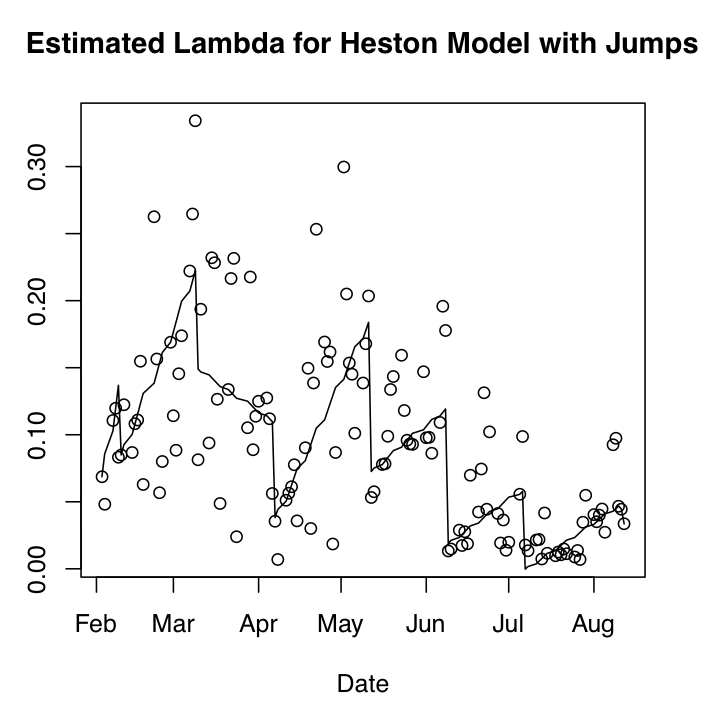
The maturity cycles in the fitted Heston model’s volatility-of-volatility can be seen further in Figure 12, where the daily estimates of $\kappa$ and $\gamma$ are shown along with an LAD fit to highlight the rate at which the parameters increase. It should be remarked that $\kappa$ exhibits a maturity cycle in-part because we’ve enforced the Feller condition in parameter estimation; $\gamma^{2}\leq 2\bar{X}\kappa$ and so periodic increases in $\gamma$ result in periodic increases in $\kappa$ .

When we include jumps, the maturity cycles disappear in the both $\widehat{\phi}_{n}$ and the diffusion parameters. However, the fitted values of the jump intensity $\lambda_{J}$ exhibit some evidence of maturity cycles, as we see in Figure 13, but these cycles are not as prevalent as those in Figures 11 or 12. Intuitively, it makes sense that increases in the jump intensity would handle little-t effects caused by short time-to-maturity, because jumps have a lot of explanatory power for options with short time-to-maturity. Since we know that little-t behavior exists and is present in the data, it must be implied into the fit in some way or another. Therefore, we must assume that maturity cycles are present in the jump model’s fitted parameters and/or $\widehat{\phi}_{n}$ , but that we are simply not able to see them. Thus, the jump model has buried the maturity cycles, and perhaps over fitting has occurred.

4.3 Comparison With VIX

Another important piece of analysis is the comparison of our fitted stochastic volatility to the VIX. For a fixed time period of length $\tau^{*}>0$ , let $QV_{t,\tau^{*}}$ denote quadratic variation,

QV_{t,\tau^{*}}\doteq\lim_{|p|\searrow 0}\sum_{t_{i}\in[t,t+\tau^{*})}\log(S_{t_{i+1}}/S_{t_{i}})^{2}=\int_{t}^{t+\tau^{*}}X_{s}ds+\sum_{i=\mathcal{Z}_{t}}^{\mathcal{Z}_{t+\tau^{*}}}\left(\log(1+J_{i})\right)^{2}\ ,

where the limit holds in probability as $|p|\doteq\sup_{i}(t_{i+1}-t_{i})\rightarrow 0$ . Quadratic variation divided by $\tau^{*}$ is the continuous time analogue of the floating-leg for a variance swap contract, and from equation (22) and using $\widehat{\phi}_{n}$ as a proxy for the risk-neutral filter, we have the swap rate:

		$\displaystyle\frac{1}{\tau^{}}\mathbb{E}^{Q}[QV_{t_{n},\tau^{}}\|\mathcal{F}_{n}^{\Delta t}]$
		$\displaystyle=\underbrace{\bar{X}+\frac{\mathbb{E}^{Q}[X_{n}\|\mathcal{F}_{n}^{\Delta t}]-\bar{X}}{\kappa\tau^{}}\left(1-e^{-\kappa\tau^{}}\right)}_{\hbox{diffusion component}}+\underbrace{\lambda_{J}\left(\sigma_{J}^{2}+(\log(1+\mu_{J})-.5\sigma_{J}^{2})^{2}\right)}_{\hbox{jump component}}$		(24)
		$\displaystyle\approx\bar{X}+\frac{\int x\widehat{\phi}_{n}(x)dx-\bar{X}}{\kappa\tau^{}}\left(1-e^{-\kappa\tau^{}}\right)+\lambda_{J}\left(\sigma_{J}^{2}+(\log(1+\mu_{J})-.5\sigma_{J}^{2})^{2}\right)\ ,$		(25)

which sets to zero the initial cost of entry into a variance swap. Obviously, the diffusion component in equation (24) is by itself the swap rate under the Heston model (without jumps), and (24) in it’s entirety is the swap rate in the presence of jumps.

For variance swaps on SPX with $\tau^{*}=$ 30 days, a useful tool for computing the risk-neutral swap rate is the VIX index. The VIX is a volatility gauge that is computed from SPX options, and is related to the risk-neutral prediction of the 30-day variance. [15] derived the VIX formula for computing the fixed-leg of the variance swap when $dS_{t}$ has no jump component,

VIX_{t}=100\sqrt{\frac{2}{\tau^{*}}\left(\int_{F_{t,\tau^{*}}}^{\infty}\frac{\mathbb{E}^{Q}[(S_{t+\tau^{*}}-K)^{+}|\mathcal{F}_{t}^{\Delta t}]}{K^{2}}dK+\int_{0}^{F_{t,\tau^{*}}}\frac{\mathbb{E}^{Q}[(K-S_{t+\tau^{*}})^{+}|\mathcal{F}_{t}^{\Delta t}]}{K^{2}}dK\right)}\ ,

where $F_{t,\tau^{*}}$ is the forward rate on $S_{t+\tau^{*}}$ at time $t$ , and the integrands are given by the market prices of European call and put options. It has since been shown in [10] that in the presence of jumps, the risk-neutral swap rate is proportional to VIX squared plus a jump term,

		$\displaystyle\frac{1}{\tau^{}}\mathbb{E}^{Q}[QV_{t_{n},\tau^{}}\|\mathcal{F}_{n}^{\Delta t}]$
		$\displaystyle=(.01\times VIX_{n})^{2}+\frac{2}{\tau^{}}\mathbb{E}^{Q}\left[\sum_{i=\mathcal{Z}_{n}}^{\mathcal{Z}_{t_{n}+\tau^{}}}.5(\log(1+J_{i}))^{2}+\log(1+J_{i})-J_{i}\Bigg\|\mathcal{F}_{n}^{\Delta t}\right]$
		$\displaystyle=(.01\times VIX_{n})^{2}+2\lambda_{J}\left(\frac{1}{2}\left(\sigma_{J}^{2}+(\log(1+\mu_{J})-.5\sigma_{J}^{2})^{2}\right)+\log(1+\mu_{J})-\frac{1}{2}\sigma_{J}^{2}-\mu_{J}\right)$
		$\displaystyle=(.01\times VIX_{n})^{2}+\lambda_{J}\left((\log(1+\mu_{J})-.5\sigma_{J}^{2})^{2}+2\log(1+\mu_{J})-2\mu_{J}\right)\ ,$		(26)

and so a comparison of VIX to the model’s prediction of $QV$ is a meaningful diagnostic. In particular, we should see a slight margin between the two:

\frac{1}{\tau^{*}}\mathbb{E}^{Q}[QV_{t_{n},\tau^{*}}|\mathcal{F}_{n}^{\Delta t}]-(.01\times VIX_{n})^{2}

=\lambda_{J}\left((\log(1+\mu_{J})-.5\sigma_{J}^{2})^{2}+2\log(1+\mu_{J})-2\mu_{J}\right)\ ,

(27)

which is the risk premium placed on jumps. We recalibrate the model everyday, so this risk premium also evolves with time.

In Figure 14, the left-hand plot shows the time series of the VIX alongside the time series of 100 $\times$ the square-root of the diffusion component of equation (25) using $\widehat{\phi}_{n}$ implied by Heston without jumps. In the same figure, the right-hand plot is the same as the left, but uses $\widehat{\phi}_{n}$ implied by the Heston model with jumps and includes the jump components of equation(25). The Heston model without jumps appears to be more consistent with the VIX than the model with jumps, particularly in the months of June, July and August. We saw in Figure 11 that the implied density mean of $X_{n}$ was similar under both models, and so it must be that the jump model’s inconsistencies with VIX are caused by the estimated jump parameters. Empirically, it was observed in [4] and independently in [27] that there is a significant jump-risk premium in variance swaps that is not accounted for by the VIX. Indeed, from Table 8 we see that the Heston model without jumps gives a lower prediction of 30-day variance than the VIX. On the other hand, we see from the table that the Heston model with jumps predicts 30-day variance that is higher than the VIX, which indicates that the fit is picking up the jump-risk premium. However, the erratic behavior in the jump model’s variance-swap rate during the later months is confusing and difficult to explain. Hence, while we are fairly certain that the inclusion of the jumps is a good idea and we are able to see the jump-risk premium in Table 8, the right-hand plot in Figure 14 raises some concerns (which we address below).

Table 7: Variance Swap Relative Bias for the Time Series of Modeled VIX

	Heston	Heston with Jumps
$x_{0}$	-0.0594	0.1407
$d=0$	-0.0601	0.1421
$d=1$	-0.0602	0.1422
$d=2$	-0.0618	0.1430

Table 8: The relative bias for the implied density’s computation of VIX. The columns list the time series mean of

\frac{100\times\sqrt{\frac{1}{\tau^{*}}\mathbb{E}^{Q}[QV_{t_{n},\tau^{*}}|\mathcal{F}_{n}^{\Delta t}]}-VIX_{n}}{VIX_{n}}

. Each row represents the proxy of the filter

\frac{1}{\tau^{*}}\mathbb{E}^{Q}[QV_{n,\tau^{*}}|\mathcal{F}_{n}^{\Delta t}]

obtained using varying degree of regularity in

\hat{\phi}_{n}

; the row labeled ‘

x_{0}

’ has the estimates obtained using

\hat{\phi}_{n}

equal to a point-mass.

In general, jumps add more degrees of freedom to the model, and so there is expected to be a better in-sample fit to the data (which we indeed saw in the implied volatilities of Figures 9 and 10). However, additional factors should not be added gratuitously, and should have an interpretation that relates them to the stylized facts observed in the market. In Figure 14, it appears that the Heston model with jumps does a very good job of tracking the VIX during the first half of 2005, but fails to track in the later months. It is possible that the months of June, July and August have been over fit by the model, but it is equally possible that variance swap contracts entered in these months provided investors with insurance against jumps that was not provided by the VIX. Indeed, Figure 15 shows the log-difference between the right-hand side of equation (27), in which there appears to be an increase in the jump-risk premium in the later months. Nevertheless, further suspicions of over fitting comes by noticing that the jump-intensity estimates in Figure 13 are decreasing over time, while the jump-risk premium in Figure 15 is increasing; we are suspicious because the model is rich enough that there are likely to be parameterizations wherein the jump intensity increases with the jump premium.

In summary, we find that implied $\widehat{\phi}_{n}$ from both the Heston and Heston model with jumps have potential to be consistent with the VIX. The results indicate that the more parsimonious Heston model without jumps consistently underprices the variance swap, which is seen as we compare the two time series’ of the implied density’s swap rate and the VIX. When jumps are included, the variance-swap rate consistently adds a jump-risk premium during the first half of 2005, but this risk premium becomes erratic in the later months. We suspect that there has been over fitting to the data by the jump-model, but we do not contend that the jump-model is mis-specified; we simply think that the jump model during this time period has exhibited some unstable behavior that warrants further investigation.

5 Summary & Conclusions

We have used a Tykhonov regularization to invert the risk-neutral prices of derivatives, and have obtained an implied filtering density on the hidden state of volatility. The method was shown to be effective in simulations where the measurements are precise and parameters are known. The solution was also shown to be accurate in estimating the 1st and 2nd filtering moments in the presence of measurement imprecision and parameter uncertainty.

When applied to SPX data, it appears that the model’s fitted parameters and the implied density can pick up the maturity cycles in the options data, which we interpret as a volatility-uncertainty premium. Also, the fitted model parameters and the implied density’s 1st and 2nd moments for the Heston model, both with and without jumps, produce a modeled rate for 30 day variance swaps on SPX that exhibited some consistency with the VIX. Overall, we find the Heston model without jumps to be straight forward to interpret because the implied objects that are easy to interpret. In contrast, the Heston model with jumps conceals the maturity cycles and implies parameters that have a less-simple explanation, and hence, it is possible that the jump model has over fit the data.

In the future, it would be interesting to explore different types of data, such as the term structures on variance swaps or commodity futures. It would also be interesting to explore richer models, and perhaps find a way to quickly solve the inverse problem using fast algorithms. An important issue that should be addressed is the challenge of obtaining a hedging portfolio when volatility is not observed.

Table 9: Estimated Parameters for Heston Model without Jumps

date	$\kappa$	$\bar{X}$	$\gamma$	$\rho$
2/3	5.56	0.02	0.45	-0.66
2/4	6.33	0.02	0.47	-0.68
2/7	8.21	0.02	0.53	-0.67
2/8	10.47	0.02	0.57	-0.65
2/9	12.01	0.02	0.62	-0.66
2/10	4.27	0.02	0.39	-0.69
2/11	4.7	0.02	0.4	-0.68
2/14	4.51	0.02	0.4	-0.7
2/15	5.61	0.02	0.43	-0.68
2/16	6.01	0.02	0.44	-0.68
2/17	5.88	0.02	0.45	-0.66
2/18	6.37	0.02	0.47	-0.66
2/22	7.26	0.02	0.51	-0.67
2/23	6.27	0.02	0.49	-0.65
2/24	5.75	0.02	0.46	-0.64
2/25	5.87	0.02	0.46	-0.68
2/28	5.68	0.02	0.46	-0.69
3/1	5.67	0.02	0.46	-0.65
3/2	9.63	0.02	0.59	-0.65
3/3	10.09	0.02	0.6	-0.61
3/4	14.58	0.02	0.7	-0.7
3/7	17.91	0.02	0.77	-0.67
3/8	24.58	0.02	0.9	-0.67
3/9	25.59	0.02	0.93	-0.61
3/10	12.51	0.02	0.66	-0.62
3/11	4.81	0.02	0.44	-0.59
3/14	5.58	0.02	0.47	-0.61

Table 10: Estimated Parameters for Heston Model with Jumps (Equation (22))

date	$\kappa$	$\bar{X}$	$\gamma$	$\rho$	$\lambda_{J}$	$\mu_{J}$	$\sigma_{J}$
2/3	1.92	0.02	0.26	-0.67	0.07	-0.1	0.23
2/4	2.34	0.02	0.29	-0.65	0.05	-0.13	0.27
2/7	1.38	0.02	0.23	-0.68	0.11	-0.08	0.17
2/8	1.42	0.02	0.22	-0.69	0.12	-0.07	0.16
2/9	1.93	0.02	0.25	-0.71	0.08	-0.08	0.21
2/10	1.14	0.02	0.2	-0.65	0.08	-0.11	0.2
2/11	0.94	0.02	0.18	-0.68	0.12	-0.08	0.18
2/14	1.21	0.02	0.2	-0.64	0.09	-0.11	0.2
2/15	1.18	0.02	0.2	-0.66	0.11	-0.09	0.18
2/16	1.27	0.02	0.21	-0.64	0.11	-0.08	0.17
2/17	0.71	0.02	0.17	-0.65	0.15	-0.08	0.16
2/18	3.17	0.02	0.31	-0.61	0.06	-0.12	0.22
2/22	1.08	0.02	0.19	-0.71	0.26	-0.06	0.14
2/23	1.66	0.02	0.24	-0.59	0.16	-0.09	0.15
2/24	2.87	0.02	0.31	-0.6	0.06	-0.12	0.24
2/25	1.94	0.02	0.26	-0.62	0.08	-0.09	0.19
2/28	0.85	0.02	0.17	-0.61	0.17	-0.1	0.16
3/1	1.48	0.02	0.23	-0.6	0.11	-0.09	0.17
3/2	2.2	0.02	0.27	-0.6	0.09	-0.09	0.21
3/3	1.36	0.02	0.22	-0.6	0.15	-0.08	0.17
3/4	2.88	0.02	0.3	-0.58	0.17	-0.07	0.15
3/7	1.73	0.02	0.24	-0.57	0.22	-0.07	0.13
3/8	1.46	0.02	0.22	-0.62	0.26	-0.05	0.12
3/9	1.49	0.02	0.22	-0.64	0.33	-0.05	0.11
3/10	2.32	0.02	0.25	-0.58	0.08	-0.11	0.23
3/11	0.7	0.02	0.16	-0.66	0.19	-0.07	0.17
3/14	2.28	0.02	0.25	-0.61	0.09	-0.1	0.22

References

[1] Y. Achdou and O. Pironneau. Computational Methods for Option Pricing. SIAM Press, Philadelphia, PA, 2005.
[2] S.I. Aihara, A. Bagchi, and S. Saha. On parameter estimation of stochastic volatility models from stock data using particle filter - application to aex index-. International Journal of Innovative Computing, Information and Control, 5(1):17–27, January 2009.
[3] Y. Aït-Sahalia. Transition densities for interest rate and other derivatives. The Journal of Finance, 54(4):1361–1395, 1999.
[4] Y. Aït-Sahalia, M. Karaman, and L. Mancini. Variance swap, risk premiums, and expectation hypothesis. 2011. Princeton-Laussane Conference, May 2011, Available at: http://ssrn.com/abstract=2136820.
[5] H. Albrecher, P. Mayer, W. Schoutens, and J. Tistaert. The little Heston trap. Wilmott Magazine, pages 83–92, January 2007.
[6] G. Bakshi, C. Cao, and Z. Chen. Empirical performance of alternative option pricing models. The Journal of Finance, 52(5):2003–2049, 1997.
[7] T. Bjork. Arbitrage Theory in Continuous Time. Oxford University Press, Oxford, UK, 2nd edition, 2000.
[8] P. Carr and R. Lee. Robust replication of volatility derivatives. In MFA 2008 Annual Meeting, 2009. PRMIA award for Best Paper in Derivatives.
[9] Peter Carr and Dilip Madan. Option valuation and the fast fourier transform. Journal of Computational Finance, 2(4):61 –73, 1999.
[10] Peter Carr and Liuren Wu. Variance risk premiums. The Review of Financial Studies, 22:1311–1341, March 2009.
[11] P. Christoffersen, K. Jacobs, and K. Mimouni. Volatility dynamics for the s&p500: Evidence from realized volatility, daily returns and option prices. In EFA 2007 Ljubljana Meetings Paper; AFA 2008 New Orleans Meetings Paper, 2007. Available at: http://ssrn.com/abstract=926373.
[12] P. Christofferson, S. Heston, and K. Jacobs. The shape and term structure of the index option smirk: Why multi-factor stochastic volatility models work so well. Management Science, 55:1914–1932, 2009.
[13] R. Cont and P. Tankov. Retrieving lévy processes from options prices: Regularization of an ill-posed inverse problem. Siam J. on Control Optimization, 45(1):1–25, 2006.
[14] J. Cvitanić, R. Lipster, and B. Rozovsky. A filtering approach to tracking volatility from prices observed at random times. Annals of Applied Probability, 16:1633–1652, 2006.
[15] Kresimir Demeterfi, Emanuel Derman, Michael Kamal, and Joseph Zou. More than you ever wanted to know about volatility swaps. The Journal of Derivatives, 6(4):9–32, 1999.
[16] R. Desai, T. Lele, and F. Viens. A monte-carlo method for portfolio optimization under partially observed stochastic volatility. In Computational Intelligence for Financial Engineering, 2003. Proceedings. 2003 IEEE International Conference on, pages 257–263, 2003.
[17] A. Drăgulescu and V. Yakovenko. Probability distribution of returns in the Heston model with stochastic volatility. Quantitative Finance, 2:443–453, 2002.
[18] B. Eraker. Do stock prices and volatility jump? reconciling evidence from spot and options prices. The Journal of Finance, 59(3):1367–1404, 2004.
[19] S. Figlewski. Estimating the implied risk neutral density for the u.s. market portfolio. In Volatility and Time Series Analysis: Essays in Honor of Robert F. Engle, Oxford, UK, 2008. Oxford University Press.
[20] Jean-Pierre Fouque, George Papanicolaou, Ronnie Sircar, and Knut Solna. Multiscale Stochastic Volatility for Equity, Interest Rate, and Credit Derivatives. Cambridge University Press, New York, NY, 2011.
[21] J.P. Fouque, G. Papanicolaou, and R. Sircar. Maturity cycles in implied volatility. Finance and Stochastics, 8:451–477, 2004.
[22] P. Friz and J. Gatheral. Valuation of volatility derivatives as an inverse problem. Quantitative Finance, 5(6):531–542, 2005.
[23] S. Heston. A closed-form solution for options with stochastic volatility with applications to bond and currency options. The Review of Financial Studies, 6(2):327–343, 1993.
[24] Arthur E. Hoerl and Robert W. Kennard. Ridge regression: Biased estimation for nonorthogonal problems. Technometrics, 12(1):pp. 55–67, 1970.
[25] A. L. Lewis. Option Valuation under Stochastic Volatility with Mathematica Code. Finance Press, Newport Beach, Ca, 2000.
[26] Eric Renault and Nizar Touzi. Option hedging and implied volatilities in a stochastic volatility model. Mathematical Finance, 6(3):279–302, 1996.
[27] V. Todorov. Variance risk premium dynamics: The role of jumps. Review of Financial Studies, 23(1):345–383, 2010.

		$\displaystyle\mbox{P}^{\Delta t}(y,x\|S_{n-1},v)$
		$\displaystyle=\frac{\partial}{\partial y}\int_{0}^{y}\mbox{P}^{\Delta t}(z,x\|S_{n-1},v)dz$
		$\displaystyle=\frac{\partial}{\partial y}\mathbb{P}(S_{n}\leq y\|X_{n}=x,X_{n-1}=v,S_{n-1})\Gamma^{\Delta t}(x\|v)$
		$\displaystyle=\frac{\partial}{\partial y}\mathbb{E}\left\{\mathbf{1}_{S_{n}\leq y}\Big\|X_{n}=x,X_{n-1}=v,S_{n-1}\right\}\Gamma^{\Delta t}(x\|v)$
		$\displaystyle=\frac{\partial}{\partial y}\mathbb{E}\left[\mathbb{E}\left\{\mathbf{1}_{S_{n}\leq y}\Big\|(X_{u})_{\{t_{n-1}\leq u\leq t_{n}\}},S_{n-1}\right\}\Big\|X_{n}=x,X_{n-1}=v,S_{n},S_{n-1}\right]\Gamma^{\Delta t}(x\|v)$
		$\displaystyle=\mathbb{E}\left[\frac{\partial}{\partial y}\mathbb{E}\left\{\mathbf{1}_{S_{n}\leq y}\Big\|(X_{u})_{\{t_{n-1}\leq u\leq t_{n}\}},S_{n-1}\right\}\Big\|X_{n}=x,X_{n-1}=v,S_{n},S_{n-1}\right]\Gamma^{\Delta t}(x\|v)$
		$\displaystyle\propto\mathbb{E}\left[\mathbb{L}(y\|(X_{u})_{\{t_{n-1}\leq u\leq t_{n}\}},S_{n-1})\Big\|X_{n}=x,X_{n-1}=v,S_{n-1}\right]\Gamma^{\Delta t}(x\|v)\ .$

		$\displaystyle\frac{1}{\tau^{}}\mathbb{E}^{Q}[QV_{t_{n},\tau^{}}\|\mathcal{F}_{n}^{\Delta t}]$
		$\displaystyle=\underbrace{\bar{X}+\frac{\mathbb{E}^{Q}[X_{n}\|\mathcal{F}_{n}^{\Delta t}]-\bar{X}}{\kappa\tau^{}}\left(1-e^{-\kappa\tau^{}}\right)}_{\hbox{diffusion component}}+\underbrace{\lambda_{J}\left(\sigma_{J}^{2}+(\log(1+\mu_{J})-.5\sigma_{J}^{2})^{2}\right)}_{\hbox{jump component}}$		(24)
		$\displaystyle\approx\bar{X}+\frac{\int x\widehat{\phi}_{n}(x)dx-\bar{X}}{\kappa\tau^{}}\left(1-e^{-\kappa\tau^{}}\right)+\lambda_{J}\left(\sigma_{J}^{2}+(\log(1+\mu_{J})-.5\sigma_{J}^{2})^{2}\right)\ ,$		(25)