跳到论文正文
W Papers独立论文阅读器 arXiv:1203.6630 论文正文 计算阅读时间 · 0%
引用这篇论文根据当前论文元数据生成,正式投稿前建议核对。


License: arXiv.org perpetual non-exclusive license
arXiv:1203.6630v2 [cs.IT] 26 Sep 2012

Power Allocation over Two Identical Gilbert-Elliott Channels

Junhua Tang Affiliation: School of Electronic Information
and Electrical Engineering
Shanghai Jiao Tong University, China
Email: junhuatang@sjtu.edu.cn
   Parisa Mansourifard Affiliation: Ming Hsieh Department
of Electrical Engineering
Viterbi School of Engineering
University of Southern California
Email: parisama@usc.edu
   Bhaskar Krishnamachari Affiliation: Ming Hsieh Department
of Electrical Engineering
Viterbi School of Engineering
University of Southern California
Email: bkrishna@usc.edu
Abstract

We study the problem of power allocation over two identical Gilbert-Elliot communication channels. Our goal is to maximize the expected discounted number of bits transmitted over an infinite time horizon. This is achieved by choosing among three possible strategies: (1) betting on channel 1 by allocating all the power to this channel, which results in high data rate if channel 1 happens to be in good state, and zero bits transmitted if channel 1 is in bad state (even if channel 2 is in good state) (2) betting on channel 2 by allocating all the power to the second channel, and (3) a balanced strategy whereby each channel is allocated half the total power, with the effect that each channel can transmit a low data rate if it is in good state. We assume that each channel’s state is only revealed upon transmission of data on that channel. We model this problem as a partially observable Markov decision processes (MDP), and derive key threshold properties of the optimal policy. Further, we show that by formulating and solving a relevant linear program the thresholds can be determined numerically when system parameters are known.

I Introduction

Adaptive power control is an important technique to select the transmission power of a wireless system according to channel condition to achieve better network performance in terms of higher data rate or spectrum efficiency [1], [2]. While there has been some recent work on power allocation over stochastic channels [3, 4, 5], the problem of optimal adaptive power allocation across multiple stochastic channels with memory is challenging and poorly understood. In this paper, we analyze a simple but fundamental problem. We consider a wireless system operating on two stochastically identical independent parallel transmission channels, each modeled as a slotted Gilber-Elliott channel (i.e. described by two-state Markov chains, with a bad state “0” and a good state “1”). Our objective is to allocate the limited power budget to the two channels dynamically so as to maximize the expected discounted number of bits transmitted over time. Since the channel state is unknown when power allocation decision is made, this problem is more challenging than it looks like.

Recently, several works have explored different sequential decision-making problems involving Gilbert-Elliott channels [6], [7], [8], [9], [10]. In [6], [7], the authors consider selecting one channel to sense/access at each time among several identical channels, formulate it as a restless multi-armed problem, and show that a simple myopic policy is optimal whenever the channels are positively correlated over time. In [8], the authors study the problem of dynamically choosing one of three transmitting schemes for a single Gilbert-Elliott channel in an attempt to maximize the expected discounted number of bits transmitted. And in [9], the authors study the problem of choosing a transmitting strategy from two choices emphasizing the case when the channel transition probabilities are unknown. While similar in spirit to these two studies, our work addresses a more challenging setting involving two independent channels. A more related two-channel problem is studied in [10], which characterizes the optimal policy to opportunistically access two non-identical Gilber-Elliott channels (generalizing the prior work on sensing policies for identical channels [6], [7]). While we address only identical channels in this work, the strategy space explored here is richer because in our formulation of power allocation, it is possible to use both channels simultaneously whilst in [6], [7], [10] only one channel is accessed in each time slot.

In this paper, we formulate our power allocation problem as a partially observable Markov decision process (POMDP). We then treat the POMDP as a continuous state MDP and develop the structure of the optimal policy (decision). Our main contributions are the following: (1) we formulate the problem of dynamic power allocation over parallel Markovian channels, (2) using the MDP theory, we theoretically prove key threshold properties of the optimal policy for this particular problem, (3) through simulation based on linear programming, we demonstrate the existence of the 0-threshold and 2-threshold structures of the optimal policy, and (4) we demonstrate how to numerically compute the thresholds and construct the optimal policy when system parameters are known.

II Problem Formulation

A. Channel model and assumptions

We consider a wireless communication system operating on two parallel channels. Each channel is described by a slotted Gilbert-Elliott model which is a one dimensional Markov chain Gi,t​(i∈{1,2},t∈{1,2,…,∞})G_{i,t}(i\in\{1,2\},t\in\{1,2,...,\infty\}) with two states: a good state denoted by 1 and a bad state denoted by 0 (ii is the channel number and tt is the time slot). The channel transition probabilities are given by P​r​[Gi,t=1|Gi,t−1=1]=λ1,i∈{1,2}Pr[G_{i,t}=1|G_{i,t-1}=1]=\lambda_{1},i\in\{1,2\} and P​r​[Gi,t=1|Gi,t−1=0]=λ0,i∈{1,2}Pr[G_{i,t}=1|G_{i,t-1}=0]=\lambda_{0},i\in\{1,2\}. We assume the two channels are identical and independent of each other, and channel transitions occur at the beginning of each time slot. We also assume that λ0≤λ1\lambda_{0}\leq\lambda_{1}, which is the positive correlation assumption commonly used in the literature.

The system has a total transmission power of PP. At the beginning of time slot tt, the system allocates transmission power P1​(t)P_{1}(t) to channel 1 and P2​(t)P_{2}(t) to channel 2, where P1​(t)+P2​(t)=PP_{1}(t)+P_{2}(t)=P. We assume the channel state is not directly observable at the beginning of each time slot. That is, the system needs to allocate the transmission power to the two parallel channels without knowing the channel states. If channel i⁡(i∈{1,2})i(i\in\{1,2\}) is used at time slot tt by allocating transmission power Pi​(t)P_{i}(t) on it, the channel state of the elapsed slot is revealed at the end of the time slot through channel feedback. But if a channel is not used, that is, if transmission power is 0 on that channel, the channel state of the elapsed slot remains unknown at the end of that slot.

B. Power allocation strategies

To simplify the problem, we assume the system may allocate one of the following three power levels to a channel: 0,P/20,P/2, or PP. That is, based on the belief in the channel state of channel ii for the current time slot tt, the system may decide to give up the channel (Pi​(t)=0P_{i}(t)=0), use it moderately (Pi​(t)=P/2P_{i}(t)=P/2) or use it fully(Pi​(t)=PP_{i}(t)=P). Since the channel state is not directly observable when the power allocation is done, the following circumstances may occur. If a channel is in bad state, no data is transmitted at all no matter what the allocated power is. If a channel is in good state, and power P/2P/2 is allocated to it, it can transmit RlR_{l} bits of data successfully during that slot. If a channel is in good condition and power PP is allocated to it, it can transmit RhR_{h} bits of data successfully during that slot. We assume Rl<Rh<2​RlR_{l}<R_{h}<2R_{l}.

We define three power allocation strategies(actions): balanced, betting on channel 1, and betting on channel 2. Each strategy is explained in detail as follows.

Balanced: For this action (denoted by BbB_{b}), the system allocates the transmission power evenly on both channels, that is, P1​(t)=P2​(t)=P/2P_{1}(t)=P_{2}(t)=P/2, for time slot tt. This corresponds to the situation when the system cannot determine which of the channels is more likely to be in good state, so it decides to “play safe” by using both of the channels.

Betting on channel 1: For this action (denoted by B1B_{1}), the system decides to “gamble” and allocate all the transmission power to channel 1. That is, P1​(t)=P,P2​(t)=0P_{1}(t)=P,P_{2}(t)=0 for time slot tt. This corresponds to the situation when the system believes that channel 1 is in a good state and channel 2 is in a bad state.

Betting on channel 2: For this action (denoted by B2B_{2}), the system put all the transmission power in channel 2, that is, P2​(t)=P,P1​(t)=0P_{2}(t)=P,P_{1}(t)=0 for time slot tt.

Note that for strategies B1B_{1} and B2B_{2}, if a channel is not used, the system (transmitter) will not acquire any knowledge about the state of that channel during the elapsed slot.

C. POMDP formulation

At the beginning of a time slot, the system is confronted with a choice among three actions. It must judiciously select actions so as to maximize the total expected discounted number of bits transmitted over an infinite time span. Because the state of the channels is not directly observable, the problem in hand is a Partially Observable Markov Decision Process (POMDP). In [11], it is shown that a sufficient statistic for determining the optimal policy is the conditional probability that the channel is in the good state at the beginning of the current slot given the past history (henceforth called belief) [8]. Denote the belief of the system by a two dimension vector 𝐱t\mathbf{x}_{t}=(x1,t,x2,t)(x_{1,t},x_{2,t}), where x1,t=Pr⁡[G1,t=1|ℏt]x_{1,t}=\Pr[G_{1,t}=1|\hbar_{t}], x2,t=Pr⁡[G2,t=1|ℏt]x_{2,t}=\Pr[G_{2,t}=1|\hbar_{t}], where ℏt\hbar_{t} is all the history of actions and observations at the current slot tt. By using this belief as the decision variable, the POMDP problem is converted into an MDP with the uncountable state space ([0,1],[0,1])([0,1],[0,1]) [8].

Define a policy π\pi as a rule that dictates the action to choose, i.e., a map from the belief at a particular time to an action in the action space. Let Vπ​(𝐩)V^{\pi}(\mathbf{p}) be the expected discounted reward with initial belief 𝐩=(p1,p2)\mathbf{p}=(p_{1},p_{2}), that is, x1,0=Pr⁡[G1,0=1|ℏ0]=p1x_{1,0}=\Pr[G_{1,0}=1|\hbar_{0}]=p_{1}, x2,0=Pr⁡[G2,0=1|ℏ0]=p2x_{2,0}=\Pr[G_{2,0}=1|\hbar_{0}]=p_{2}, where the superscript π\pi denotes the policy being followed. Define β(∈[0,1))\beta(\in[0,1)) as the discount factor, the expected discounted reward has the following expression

Vπ​(𝐩)=Eπ​[∑t=0∞βt​gat​(𝐱t)|𝐱0=𝐩],V^{\pi}(\mathbf{p})=E_{\pi}[\sum_{t=0}^{\infty}\beta^{t}g_{a_{t}}(\mathbf{x}_{t})|\mathbf{x}_{0}=\mathbf{p}], (1)

where EπE_{\pi} represents the expectation given that the policy π\pi is employed, tt is the time slot index, ata_{t} is the action chosen at time tt, at∈{Bb,B1,B2}a_{t}\in\{B_{b},B_{1},B_{2}\}. The term gat​(𝐱t)g_{a_{t}}(\mathbf{x}_{t}) denotes the expected reward acquired when the belief is 𝐱𝐭\mathbf{x_{t}} and the action ata_{t} is chosen:

gat​(𝐱t)={x1,t​Rl+x2,t​Rl,ifat=Bbx1,t​Rh,ifat=B1x2,t​Rh,ifat=B2.g_{a_{t}}(\mathbf{x}_{t})=\left\{\begin{array}[]{rl}x_{1,t}R_{l}+x_{2,t}R_{l},&\quad\mbox{if}\quad a_{t}=B_{b}\\ x_{1,t}R_{h},&\quad\mbox{if}\quad a_{t}=B_{1}\\ x_{2,t}R_{h},&\quad\mbox{if}\quad a_{t}=B_{2}\\ \end{array}.\right.
(2)

Now we define the value function V⁡(𝐩)V(\mathbf{p}) as

V⁡(𝐩)=maxπ⁡Vπ​(𝐩),for all𝐩∈([0,1],[0,1]).V(\mathbf{p})=\max_{\pi}V^{\pi}(\mathbf{p}),\quad\mbox{for all}\quad\mathbf{p}\in([0,1],[0,1]). (3)

A policy is said to be stationary if it is a function mapping the state space ([0,1],[0,1])([0,1],[0,1]) into the action space {Bb,B1,B2}\{B_{b},B_{1},B_{2}\}. Ross proved in [12] (Th.6.3) that there exists a stationary policy π∗\pi^{*} such that V​(𝐩)=Vπ∗​(𝐩)V(\mathbf{p})=V^{\pi^{*}}(\mathbf{p}). The value function V⁡(𝐩)V(\mathbf{p}) satisfies the Bellman equation

V⁡(𝐩)=maxa∈{Bb,B1,B2}⁡{Va​(𝐩)},V(\mathbf{p})=\max_{a\in\{B_{b},B_{1},B_{2}\}}\{V_{a}(\mathbf{p})\}, (4)

where Va​(𝐩)V_{a}(\mathbf{p}) is the value acquired by taking action aa when the initial belief is 𝐩\mathbf{p}. Va​(𝐩)V_{a}(\mathbf{p}) is given by

Va(𝐩)=ga(𝐩)+βE𝐲[V(𝐲)|𝐱0=𝐩,a0=a],V_{a}(\mathbf{p})=g_{a}(\mathbf{p})+\beta E^{\mathbf{y}}[V(\mathbf{y})|\mathbf{x}_{0}=\mathbf{p},a_{0}=a], (5)

where 𝐲\mathbf{y} denotes the next belief when the action aa is chosen and the initial belief is 𝐩\mathbf{p}. The term Va​(𝐩)V_{a}(\mathbf{p}) is explained next for the three possible actions.

a) Balanced (action BbB_{b}): If this action is taken, and the current belief is 𝐩=(p1,p2)\mathbf{p}=(p_{1},p_{2}), the immediate reward is p1​Rl+p2​Rlp_{1}R_{l}+p_{2}R_{l}. Since both channels are used, the channel quality of both channels during the current slot is then revealed to the transmitter. With probability p1p_{1} the first channel will be in good state and hence the belief of channel 1 at the beginning of the next slot will be λ1\lambda_{1}. Likewise, with probability 1−p11-p_{1} channel 1 will turn out to be in bad state and hence the updated belief of channel 1 for the next slot is λ0\lambda_{0}. Since channel 2 and channel 1 are identical, channel 2 has similar belief update. Consequently if action BbB_{b} is taken, the value function evolves as

VBb​(p1,p2)\displaystyle V_{B_{b}}(p_{1},p_{2}) (6)
=\displaystyle= p1Rl+p2Rl+β[(1−p1)(1−p2)V(λ0,λ0)\displaystyle p_{1}R_{l}+p_{2}R_{l}+\beta[(1-p_{1})(1-p_{2})V(\lambda_{0},\lambda_{0})
+\displaystyle+ p1​(1−p2)​V​(λ1,λ0)+(1−p1)​p2​V​(λ0,λ1)\displaystyle p_{1}(1-p_{2})V(\lambda_{1},\lambda_{0})+(1-p_{1})p_{2}V(\lambda_{0},\lambda_{1})
+\displaystyle+ p1p2V(λ1,λ1)].\displaystyle p_{1}p_{2}V(\lambda_{1},\lambda_{1})].

b) Betting on channel 1( action B1B_{1}): If this action is taken, and the current belief is 𝐩=(p1,p2)\mathbf{p}=(p_{1},p_{2}), the immediate reward is p1​Rhp_{1}R_{h}. But since channel 2 is not used, its channel state remains unknown. Hence if the belief of channel 2 during the elapsed time slot is p2p_{2}, its belief at the beginning of the next time slot is given by

T⁡(p2)=p2​λ1+(1−p2)​λ0=α​p2+λ0,T(p_{2})=p_{2}\lambda_{1}+(1-p_{2})\lambda_{0}=\alpha p_{2}+\lambda_{0}, (7)

where α=λ1−λ0\alpha=\lambda_{1}-\lambda_{0}. Consequently, if this action is taken, the value function evolves as

VB1​(p1,p2)=p1​Rh+\displaystyle V_{B_{1}}(p_{1},p_{2})=p_{1}R_{h}+
β⁡[(1−p1)​V​(λ0,T⁡(p2))+p1​V​(λ1,T⁡(p2))].\displaystyle\beta[(1-p_{1})V(\lambda_{0},T(p_{2}))+p_{1}V(\lambda_{1},T(p_{2}))]. (8)

c) Betting on channel 2(action B2B_{2}): Similar to action B1B_{1}, if action B2B_{2} is taken, the value function evolves as

VB2​(p1,p2)=p2​Rh+\displaystyle V_{B_{2}}(p_{1},p_{2})=p_{2}R_{h}+
β⁡[(1−p2)​V​(T⁡(p1),λ0)+p2​V​(T⁡(p1),λ1)],\displaystyle\beta[(1-p_{2})V(T(p_{1}),\lambda_{0})+p_{2}V(T(p_{1}),\lambda_{1})], (9)

where

T⁡(p1)=p1​λ1+(1−p1)​λ0=α​p1+λ0.T(p_{1})=p_{1}\lambda_{1}+(1-p_{1})\lambda_{0}=\alpha p_{1}+\lambda_{0}. (10)

Finally the Bellman equation for our power allocation problem reads as follows

V⁡(𝐩)=max⁡{VBb​(𝐩),VB1​(𝐩),VB2​(𝐩)}.V(\mathbf{p})=\max\{V_{B_{b}}(\mathbf{p}),V_{B_{1}}(\mathbf{p}),V_{B_{2}}(\mathbf{p})\}. (11)

III Structure of the Optimal Policy

From the above discussion we understand that an optimal policy exists for our power allocation problem. In this section, we try to derive the optimal policy by first looking at the features of its structure.

A: Properties of value function

Lemma 1.

VBi​(p1,p2),i∈{1,2,b}V_{B_{i}}(p_{1},p_{2}),i\in\{1,2,b\} is affine with respect to p1p_{1} and p2p_{2} and the following equalities hold:

VBi​(c​p+(1−c)​p′,p2)=c​VBi​(p,p2)+(1−c)​VBi​(p′,p2),\displaystyle V_{B_{i}}(cp+(1-c)p^{\prime},p_{2})=cV_{B_{i}}(p,p_{2})+(1-c)V_{B_{i}}(p^{\prime},p_{2}),
VBi​(p1,c​p+(1−c)​p′)=c​VBi​(p1,p)+(1−c)​VBi​(p1,p′),\displaystyle V_{B_{i}}(p_{1},cp+(1-c)p^{\prime})=cV_{B_{i}}(p_{1},p)+(1-c)V_{B_{i}}(p_{1},p^{\prime}), (12)

where 0≤c≤10\leq c\leq 1 is a constant; and we say f⁡(x)f(x) is affine with respect to xx if f⁡(x)=a+c​xf(x)=a+cx, with constant aa and cc.

Proof.

It is clear that VBbV_{B_{b}} is affine in p1p_{1} and p2p_{2} from (6). It is also obvious that VB1V_{B_{1}} is affine in p1p_{1} and VB2V_{B_{2}} is affine in p2p_{2} from (8) and (9). Next we will prove that VB1V_{B_{1}} is affine in p2p_{2} and VB2V_{B_{2}} is affine in p1p_{1}, which will make the proof complete.

Now we prove that VB1V_{B_{1}} is affine in p2p_{2}. We will first show that the second term on the right side of (8) is affine in p2p_{2}, the third term can then be shown to be affine in p2p_{2} in a similar manner, thus the summation of the three terms in (8) is affine in p2p_{2}.

Now let us look at the second term on the right side of (8), the main part V⁡(λ0,T⁡(p2))V(\lambda_{0},T(p_{2})) is one of the following three forms: VBb​(λ0,T⁡(p2))V_{B_{b}}(\lambda_{0},T(p_{2})), VB2​(λ0,T⁡(p2))V_{B_{2}}(\lambda_{0},T(p_{2})), or VB1​(λ0,T⁡(p2))V_{B_{1}}(\lambda_{0},T(p_{2})). The first form VBb​(λ0,T⁡(p2))V_{B_{b}}(\lambda_{0},T(p_{2})) is affine in p2p_{2} because VBb​(λ0,T⁡(p2))V_{B_{b}}(\lambda_{0},T(p_{2})) is affine in T⁡(p2)T(p_{2}) and T⁡(p2)=α​p2+λ0T(p_{2})=\alpha p_{2}+\lambda_{0} is affine in p2p_{2}. Similarly, the second form VB2​(λ0,T⁡(p2))V_{B_{2}}(\lambda_{0},T(p_{2})) is affine in T⁡(p2)T(p_{2}) thus affine in p2p_{2}. The third form VB1​(λ0,T⁡(p2))V_{B_{1}}(\lambda_{0},T(p_{2})) is written as:

VB1​(λ0,T⁡(p2))\displaystyle V_{B_{1}}(\lambda_{0},T(p_{2}))
=λ0​Rh+β​λ0​V​(λ1,T2​(p2))+β⁡(1−λ0)​V​(λ0,T2​(p2)),\displaystyle=\lambda_{0}R_{h}+\beta\lambda_{0}V(\lambda_{1},T^{2}(p_{2}))+\beta(1-\lambda_{0})V(\lambda_{0},T^{2}(p_{2})),

where Tn​(p)=T⁡(Tn−1​(p))=λ01−α​(1−αn)+αn​pT^{n}(p)=T(T^{n-1}(p))=\frac{\lambda_{0}}{1-\alpha}(1-\alpha^{n})+\alpha^{n}p. Since Tn​(p2)T^{n}(p_{2}) is affine in p2p_{2}, (III) is affine in p2p_{2} as soon as V⁡(λ1,Tn​(p2))V(\lambda_{1},T^{n}(p_{2})) takes the form of VBb​(λ1,Tn​(p2))V_{B_{b}}(\lambda_{1},T^{n}(p_{2})) or VB2​(λ1,Tn​(p2))V_{B_{2}}(\lambda_{1},T^{n}(p_{2})), and V⁡(λ0,T2​(p2))V(\lambda_{0},T^{2}(p_{2})) takes the form of VBb​(λ0,Tn​(p2))V_{B_{b}}(\lambda_{0},T^{n}(p_{2})) or VB2​(λ0,Tn​(p2))V_{B_{2}}(\lambda_{0},T^{n}(p_{2})), n=2,3,4,…n=2,3,4,..., which is affine in p2p_{2}. If V⁡(λ1,Tn​(p2))V(\lambda_{1},T^{n}(p_{2})) continues to take the form VB1​(λ1,Tn​(p2))V_{B_{1}}(\lambda_{1},T^{n}(p_{2})) till nn goes to infinity, V⁡(λ1,Tn​(p2))V(\lambda_{1},T^{n}(p_{2})) will eventually become a constant V⁡(λ1,λ01−α)V(\lambda_{1},\frac{\lambda_{0}}{1-\alpha}) because Tn​(p2)→λ01−α,n→∞T^{n}(p_{2})\rightarrow\frac{\lambda_{0}}{1-\alpha},n\rightarrow\infty. Which means a special case of affine linearity in p2p_{2}. With this we show that the third form VB1​(λ0,T⁡(p2))V_{B_{1}}(\lambda_{0},T(p_{2})) is affine in p2p_{2}. Therefore we have shown that V⁡(λ0,T⁡(p2))V(\lambda_{0},T(p_{2})) is affine in p2p_{2}, thus the second term on the right side of (8) is affine in p2p_{2}.

Similarly we can show that the third term on the right side of (8) is affine in p2p_{2}, thus VB1​(p1,p2)V_{B_{1}}(p_{1},p_{2}) is affine in p2p_{2}.

The affine linearity of VB2​(p1,p2)V_{B_{2}}(p_{1},p_{2}) in p1p_{1} can be proved using the same technique and the detail is omitted due to space limit. ∎

Lemma 2.

VBi​(p1,p2),i∈{1,2,b}V_{B_{i}}(p_{1},p_{2}),i\in\{1,2,b\} is convex in p1p_{1} and p2p_{2}.

Proof.

The convexity of VBi,i∈{1,2,b}V_{B_{i}},i\in\{1,2,b\} in p1p_{1} and p2p_{2} follows from its affine linearity in Lemma 1. ∎

Lemma 3.

V⁡(p1,p2)=V⁡(p2,p1)V(p_{1},p_{2})=V(p_{2},p_{1}), that is, V⁡(p1,p2)V(p_{1},p_{2}) is symmetric with respect to the line p1=p2p_{1}=p_{2} in the belief space.

Proof.

Define Vn​(p1,p2)V^{n}(p_{1},p_{2}) as the optimal value when the decision horizon spans only nn stages. Then we have

V1​(p1,p2)\displaystyle V^{1}(p_{1},p_{2}) (14)
=\displaystyle= max⁡{VBb1​(p1,p2),VB11​(p1,p2),VB21​(p1,p2)}\displaystyle\max\{V_{B_{b}}^{1}(p_{1},p_{2}),V_{B_{1}}^{1}(p_{1},p_{2}),V_{B_{2}}^{1}(p_{1},p_{2})\}
=\displaystyle= max⁡{p1​Rl+p2​Rl,p1​Rh,p2​Rh}.\displaystyle\max\{p_{1}R_{l}+p_{2}R_{l},p_{1}R_{h},p_{2}R_{h}\}.
V1​(p2,p1)\displaystyle V^{1}(p_{2},p_{1}) (15)
=\displaystyle= max⁡{VBb1​(p2,p1),VB11​(p2,p1),VB21​(p2,p1)}\displaystyle\max\{V_{B_{b}}^{1}(p_{2},p_{1}),V_{B_{1}}^{1}(p_{2},p_{1}),V_{B_{2}}^{1}(p_{2},p_{1})\}
=\displaystyle= max⁡{p2​Rl+p1​Rl,p2​Rh,p1​Rh}.\displaystyle\max\{p_{2}R_{l}+p_{1}R_{l},p_{2}R_{h},p_{1}R_{h}\}.

It is easy to see that

V1​(p1,p2)=V1​(p2,p1).V^{1}(p_{1},p_{2})=V^{1}(p_{2},p_{1}). (16)

Assume Vk​(x1,x2)=Vk​(x2,x1),k≥1V^{k}(x_{1},x_{2})=V^{k}(x_{2},x_{1}),k\geq 1, next we will prove that Vk+1​(p1,p2)=Vk+1​(p2,p1)V^{k+1}(p_{1},p_{2})=V^{k+1}(p_{2},p_{1}).

VBbk+1​(p1,p2)\displaystyle V_{B_{b}}^{k+1}(p_{1},p_{2}) (17)
=\displaystyle= p1Rl+p2Rh+β[(1−p1)(1−p2)Vk(λ0,λ0)\displaystyle p_{1}R_{l}+p_{2}R_{h}+\beta[(1-p_{1})(1-p_{2})V^{k}(\lambda_{0},\lambda_{0})
+\displaystyle+ p1​(1−p2)​Vk​(λ1,λ0)+(1−p1)​p2​Vk​(λ0,λ1)\displaystyle p_{1}(1-p_{2})V^{k}(\lambda_{1},\lambda_{0})+(1-p_{1})p_{2}V^{k}(\lambda_{0},\lambda_{1})
+\displaystyle+ p1p2Vk(λ1,λ1)]\displaystyle p_{1}p_{2}V^{k}(\lambda_{1},\lambda_{1})]
VB1k+1​(p1,p2)=p1​Rh+\displaystyle V_{B_{1}}^{k+1}(p_{1},p_{2})=p_{1}R_{h}+
β⁡[(1−p1)​Vk​(λ0,T⁡(p2))+p1​Vk​(λ1,T⁡(p2))].\displaystyle\beta[(1-p_{1})V^{k}(\lambda_{0},T(p_{2}))+p_{1}V^{k}(\lambda_{1},T(p_{2}))]. (18)
VB2k+1​(p1,p2)=p2​Rh+\displaystyle V_{B_{2}}^{k+1}(p_{1},p_{2})=p_{2}R_{h}+
β⁡[(1−p2)​Vk​(T⁡(p1),λ0)+p2​Vk​(T⁡(p1),λ1)].\displaystyle\beta[(1-p_{2})V^{k}(T(p_{1}),\lambda_{0})+p_{2}V^{k}(T(p_{1}),\lambda_{1})]. (19)

Using the assumption that Vk​(x1,x2)=Vk​(x2,x1)V^{k}(x_{1},x_{2})=V^{k}(x_{2},x_{1}), it is easy to see that

VB1k+1​(p2,p1)\displaystyle V_{B_{1}}^{k+1}(p_{2},p_{1}) (20)
=\displaystyle= p2​Rh+β⁡[(1−p2)​Vk​(λ0,T⁡(p1))+p2​Vk​(λ1,T⁡(p1))]\displaystyle p_{2}R_{h}+\beta[(1-p_{2})V^{k}(\lambda_{0},T(p_{1}))+p_{2}V^{k}(\lambda_{1},T(p_{1}))]
=\displaystyle= p2​Rh+β⁡[(1−p2)​Vk​(T⁡(p1),λ0)+p2​Vk​(T⁡(p1),λ1)]\displaystyle p_{2}R_{h}+\beta[(1-p_{2})V^{k}(T(p_{1}),\lambda_{0})+p_{2}V^{k}(T(p_{1}),\lambda_{1})]
=\displaystyle= VB2k+1​(p1,p2)\displaystyle V_{B_{2}}^{k+1}(p_{1},p_{2})

Similarly, we have VB2k+1​(p2,p1)=VB1k+1​(p1,p2)V_{B_{2}}^{k+1}(p_{2},p_{1})=V_{B_{1}}^{k+1}(p_{1},p_{2}), and VBbk+1​(p2,p1)=VBbk+1​(p1,p2)V_{B_{b}}^{k+1}(p_{2},p_{1})=V_{B_{b}}^{k+1}(p_{1},p_{2}), thus

Vk+1​(p1,p2)\displaystyle V^{k+1}(p_{1},p_{2}) (21)
=\displaystyle= max⁡{VBbk+1​(p1,p2),VB1k+1​(p1,p2),VB2k+1​(p1,p2)}\displaystyle\max\{V_{B_{b}}^{k+1}(p_{1},p_{2}),V_{B_{1}}^{k+1}(p_{1},p_{2}),V_{B_{2}}^{k+1}(p_{1},p_{2})\}
=\displaystyle= max⁡{VBbk+1​(p2,p1),VB2k+1​(p2,p1),VB1k+1​(p2,p1)}\displaystyle\max\{V_{B_{b}}^{k+1}(p_{2},p_{1}),V_{B_{2}}^{k+1}(p_{2},p_{1}),V_{B_{1}}^{k+1}(p_{2},p_{1})\}
=\displaystyle= Vk+1​(p2,p1).\displaystyle V^{k+1}(p_{2},p_{1}).

From the theory of MDPs, we know that Vn​(p1,p2)→V⁡(p1,p2)V^{n}(p_{1},p_{2})\rightarrow V(p_{1},p_{2}) as n→∞n\rightarrow\infty. Hence we have V⁡(p1,p2)=V⁡(p2,p1)V(p_{1},p_{2})=V(p_{2},p_{1}), for any (p1,p2)(p_{1},p_{2}) in the belief space. ∎

B: Properties of the decision regions of policy π∗\pi*

We use Φa\Phi_{a} to denote the set of beliefs for which it is optimal to take the action aa. That is,

Φa={(p1,p2)∈([0,1],[0,1]),V⁡(p1,p2)=Va​(p1,p2)},\displaystyle\Phi_{a}=\{(p_{1},p_{2})\in([0,1],[0,1]),V(p_{1},p_{2})=V_{a}(p_{1},p_{2})\},
a∈{Bb,B1,B2}.\displaystyle a\in\{B_{b},B_{1},B_{2}\}. (22)
Definition 1.

Φa\Phi_{a} is said to be contiguous along p1p_{1} dimension if we have (x1,p2)∈Φa(x_{1},p_{2})\in\Phi_{a} and (x2,p2)∈Φa(x_{2},p_{2})\in\Phi_{a}, then ∀x∈[x1,x2]\forall x\in[x_{1},x_{2}], we have (x,p2)∈Φa(x,p_{2})\in\Phi_{a}. Similarly, we say Φa\Phi_{a} is contiguous along p2p_{2} dimension if we have (p1,y1)∈Φa(p_{1},y_{1})\in\Phi_{a} and (p1,y2)∈Φa(p_{1},y_{2})\in\Phi_{a}, then ∀y∈[y1,y2]\forall y\in[y_{1},y_{2}], we have (p1,y)∈Φa(p_{1},y)\in\Phi_{a}.

Theorem 1.

ΦBb\Phi_{B_{b}} is contiguous in both p1p_{1} and p2p_{2} dimensions. ΦB1\Phi_{B_{1}} is contiguous in p1p_{1} dimension, and ΦB2\Phi_{B_{2}} is contiguous in p2p_{2} dimension.

Proof.

Here we will prove the theory for ΦB​1\Phi_{B1}, and the results for ΦB2\Phi_{B_{2}} and ΦBb\Phi_{B_{b}} can be proved in a similar manner. Let (x1,p2),(x2,p2)∈ΦB1(x_{1},p_{2}),(x_{2},p_{2})\in\Phi_{B_{1}}, next we show that OPEN((c​x1+(1−c)​x2),p2))((cx_{1}+(1-c)x_{2}),p_{2})) is also in region ΦB1\Phi_{B_{1}}, where c∈[0,1]c\in[0,1].

V⁡((c​x1+(1−c)​x2),p2)\displaystyle V((cx_{1}+(1-c)x_{2}),p_{2}) (23)
≤\displaystyle\leq c​V​(x1,p2)+(1−c)​V​(x2,p2)\displaystyle cV(x_{1},p_{2})+(1-c)V(x_{2},p_{2})
=\displaystyle= c​VB1​(x1,p2)+(1−c)​VB1​(x2,p2)\displaystyle cV_{B_{1}}(x_{1},p_{2})+(1-c)V_{B_{1}}(x_{2},p_{2})
=\displaystyle= VB1​((c​x1+(1−c)​x2),p2)\displaystyle V_{B_{1}}((cx_{1}+(1-c)x_{2}),p_{2})
≤\displaystyle\leq V⁡((c​x1+(1−c)​x2),p2),\displaystyle V((cx_{1}+(1-c)x_{2}),p_{2}),

where the first inequality comes from the convexity of V⁡(p1,p2)V(p_{1},p_{2}) in p1p_{1}; the first equality follows from the fact that (x1,p2),(x2,p2)∈ΦB1(x_{1},p_{2}),(x_{2},p_{2})\in\Phi_{B_{1}}; the second equality comes from the fact that VB1V_{B_{1}} is linear in p1p_{1} as in Lemma 1; the last inequality follows from the definition of V⁡(p1,p2)V(p_{1},p_{2}). In the above equation, we have V⁡((c​x1+(1−c)​x2),p2)=VB1​((c​x1+(1−c)​x2),p2)V((cx_{1}+(1-c)x_{2}),p_{2})=V_{B_{1}}((cx_{1}+(1-c)x_{2}),p_{2}), which means OPEN(c​x1+(1−c)​x2),p2)(cx_{1}+(1-c)x_{2}),p_{2}) is in the region ΦB​1\Phi_{B1}, therefore ΦB​1\Phi_{B1} is contiguous in p1p_{1} dimension by definition 1. ∎

Theorem 2.

If belief (p1,p2)(p_{1},p_{2}) is in ΦB1\Phi_{B_{1}}, then belief (p2,p1)(p_{2},p_{1}) is in ΦB2\Phi_{B_{2}}. In other words, the decision regions of B1B_{1} and B2B_{2} are mirrors with respect to the line p1=p2p_{1}=p_{2} in the belief space.

Proof.

Let (p1,p2)(p_{1},p_{2}) be a belief state in the decision region of B1B_{1}, then we have

V⁡(p1,p2)\displaystyle V(p_{1},p_{2}) =\displaystyle= max⁡{VBb​(p1,p2),VB1​(p1,p2),VB2​(p1,p2)}\displaystyle\max\{V_{B_{b}}(p_{1},p_{2}),V_{B_{1}}(p_{1},p_{2}),V_{B_{2}}(p_{1},p_{2})\} (24)
=\displaystyle= VB1​(p1,p2).\displaystyle V_{B_{1}}(p_{1},p_{2}).

Using equations (6),(8) and (9),we have

VB1​(p1,p2)\displaystyle V_{B_{1}}(p_{1},p_{2})
=\displaystyle= p1​Rh+β⁡[(1−p1)​V​(λ0,T⁡(p2))+p1​V​(λ1,T⁡(p2))]\displaystyle p_{1}R_{h}+\beta[(1-p_{1})V(\lambda_{0},T(p_{2}))+p_{1}V(\lambda_{1},T(p_{2}))]
>\displaystyle> VB2​(p1,p2)\displaystyle V_{B_{2}}(p_{1},p_{2})
=\displaystyle= p2​Rh+β⁡[(1−p2)​V​(T⁡(p1),λ0)+p2​V​(T⁡(p1),λ1)],\displaystyle p_{2}R_{h}+\beta[(1-p_{2})V(T(p_{1}),\lambda_{0})+p_{2}V(T(p_{1}),\lambda_{1})],

and

VB1​(p1,p2)\displaystyle V_{B_{1}}(p_{1},p_{2}) (26)
>\displaystyle> VBb​(p1,p2)\displaystyle V_{B_{b}}(p_{1},p_{2})
=\displaystyle= p1Rl+p2Rl+β[(1−p1)(1−p2)V(λ0,λ0)\displaystyle p_{1}R_{l}+p_{2}R_{l}+\beta[(1-p_{1})(1-p_{2})V(\lambda_{0},\lambda_{0})
+\displaystyle+ p1​(1−p2)​V​(λ1,λ0)+(1−p1)​p2​V​(λ0,λ1)\displaystyle p_{1}(1-p_{2})V(\lambda_{1},\lambda_{0})+(1-p_{1})p_{2}V(\lambda_{0},\lambda_{1})
+\displaystyle+ p1p2V(λ1,λ1)].\displaystyle p_{1}p_{2}V(\lambda_{1},\lambda_{1})].

Now consider the belief state of (p2,p1)(p_{2},p_{1}),

VB2​(p2,p1)\displaystyle V_{B_{2}}(p_{2},p_{1}) (27)
=\displaystyle= p1​Rh+β⁡[(1−p1)​V​(T⁡(p2),λ0)+p1​V​(T⁡(p2),λ1)]\displaystyle p_{1}R_{h}+\beta[(1-p_{1})V(T(p_{2}),\lambda_{0})+p_{1}V(T(p_{2}),\lambda_{1})]
=\displaystyle= VB1​(p1,p2)\displaystyle V_{B_{1}}(p_{1},p_{2})
>\displaystyle> VB2​(p1,p2)\displaystyle V_{B_{2}}(p_{1},p_{2})
=\displaystyle= p2​Rh+β⁡[(1−p2)​V​(T⁡(p1),λ0)+p2​V​(T⁡(p1),λ1)]\displaystyle p_{2}R_{h}+\beta[(1-p_{2})V(T(p_{1}),\lambda_{0})+p_{2}V(T(p_{1}),\lambda_{1})]
=\displaystyle= VB1​(p2,p1),\displaystyle V_{B_{1}}(p_{2},p_{1}),

where the second and last equations follow by comparing the expression in equation (III) and using the fact that V⁡(p1,p2)=V⁡(p2,p1)V(p_{1},p_{2})=V(p_{2},p_{1}) (Lemma 3). Similarly, from (26) and Lemma 3, we have

VB2​(p2,p1)>VBb​(p2,p1).V_{B_{2}}(p_{2},p_{1})>V_{B_{b}}(p_{2},p_{1}). (28)

Thus we have

V⁡(p2,p1)\displaystyle V(p_{2},p_{1}) =\displaystyle= max⁡{VBb​(p2,p1),VB1​(p2,p1),VB2​(p2,p1)}\displaystyle\max\{V_{B_{b}}(p_{2},p_{1}),V_{B_{1}}(p_{2},p_{1}),V_{B_{2}}(p_{2},p_{1})\} (29)
=\displaystyle= VB2​(p2,p1),\displaystyle V_{B_{2}}(p_{2},p_{1}),

which means (p2,p1)(p_{2},p_{1}) lies in the decision region of B2B_{2}, that is, (p2,p1)∈ΦB2(p_{2},p_{1})\in\Phi_{B_{2}}. This concludes the proof. ∎

Theorem 3.

If belief (p1,p2)(p_{1},p_{2}) is in ΦBb\Phi_{B_{b}}, then belief (p2,p1)(p_{2},p_{1}) is in ΦBb\Phi_{B_{b}}. That is, the decision region of BbB_{b} is symmetric with respect to the line p1=p2p_{1}=p_{2} in the belief region.

Proof.

Suppose (p1,p2)(p_{1},p_{2}) is in ΦBb\Phi_{B_{b}}, then we have

V⁡(p1,p2)\displaystyle V(p_{1},p_{2}) =\displaystyle= max⁡{VBb​(p1,p2),VB1​(p1,p2),VB2​(p1,p2)}\displaystyle\max\{V_{B_{b}}(p_{1},p_{2}),V_{B_{1}}(p_{1},p_{2}),V_{B_{2}}(p_{1},p_{2})\} (30)
=\displaystyle= VBb​(p1,p2)\displaystyle V_{B_{b}}(p_{1},p_{2})

Now consider the belief state (p2,p1)(p_{2},p_{1}),

VBb​(p2,p1)\displaystyle V_{B_{b}}(p_{2},p_{1}) (31)
=\displaystyle= p2Rl+p1Rl+β[(1−p2)(1−p1)V(λ0,λ0)\displaystyle p_{2}R_{l}+p_{1}R_{l}+\beta[(1-p_{2})(1-p_{1})V(\lambda_{0},\lambda_{0})
+\displaystyle+ p2​(1−p1)​V​(λ1,λ0)+(1−p2)​p1​V​(λ0,λ1)\displaystyle p_{2}(1-p_{1})V(\lambda_{1},\lambda_{0})+(1-p_{2})p_{1}V(\lambda_{0},\lambda_{1})
+\displaystyle+ p2p1V(λ1,λ1)]\displaystyle p_{2}p_{1}V(\lambda_{1},\lambda_{1})]
=\displaystyle= VBb​(p1,p2)\displaystyle V_{B_{b}}(p_{1},p_{2})
>\displaystyle> VB1​(p1,p2)\displaystyle V_{B_{1}}(p_{1},p_{2})
=\displaystyle= p1​Rh+β⁡[(1−p1)​V​(λ0,T⁡(p2))+p1​V​(λ1,T⁡(p2))]\displaystyle p_{1}R_{h}+\beta[(1-p_{1})V(\lambda_{0},T(p_{2}))+p_{1}V(\lambda_{1},T(p_{2}))]
=\displaystyle= VB2​(p2,p1),\displaystyle V_{B_{2}}(p_{2},p_{1}),

where the equations follow from (6), (8), (9) and Lemma 3. The inequality comes from the assumption that (p1,p2)(p_{1},p_{2}) is in ΦBb\Phi_{B_{b}}. Similarly, we have VBb​(p2,p1)>VB1​(p2,p1)V_{B_{b}}(p_{2},p_{1})>V_{B_{1}}(p_{2},p_{1}). That is,

V⁡(p2,p1)\displaystyle V(p_{2},p_{1}) =\displaystyle= max⁡{VBb​(p2,p1),VB1​(p2,p1),VB2​(p2,p1)}\displaystyle\max\{V_{B_{b}}(p_{2},p_{1}),V_{B_{1}}(p_{2},p_{1}),V_{B_{2}}(p_{2},p_{1})\} (32)
=\displaystyle= VBb​(p2,p1).\displaystyle V_{B_{b}}(p_{2},p_{1}).

That is, (p2,p1)(p_{2},p_{1}) is in ΦBb\Phi_{B_{b}}. And this concludes the proof. ∎

Lemma 4.

After each channel is used once, the belief state is the four sides of a rectangle determined by four vertices at (λ0,λ0),(λ0,λ1),(λ1,λ0),(λ1,λ1)(\lambda_{0},\lambda_{0}),(\lambda_{0},\lambda_{1}),(\lambda_{1},\lambda_{0}),(\lambda_{1},\lambda_{1}) (Figure 1 (a)).

Proof.

From the belief update in (6)(8)(9), it is clear that the belief state of a channel is updated to one of the following three values after any action: λ0\lambda_{0}, λ1\lambda_{1}, or T⁡(p)T(p), where pp is the current belief of a channel. For any 0≤p≤10\leq p\leq 1, λ0≤T⁡(p)=λ0+(λ1−λ0)​p≤λ1\lambda_{0}\leq T(p)=\lambda_{0}+(\lambda_{1}-\lambda_{0})p\leq\lambda_{1}. Therefore the belief state of a channel is between λ0\lambda_{0} and λ1\lambda_{1}.

Furthermore, since at least one channel is used in our power allocation strategy, its channel state is revealed at the end of the time slot. This means at least one of the channel has a belief of either λ0\lambda_{0} or λ1\lambda_{1}. And this concludes the proof. ∎

Refer to caption
Fig. 1: (a) The feasible belief space. (b) The threshold on p1p_{1} ( p2=λ0​(λ1CLOSEp_{2}=\lambda_{0}(\lambda_{1})).
Theorem 4.

Let p1∈[λ0,λ1]p_{1}\in[\lambda_{0},\lambda_{1}], p2=λ0p_{2}=\lambda_{0}, there exists a threshold ρ1\rho_{1}(λ0≤ρ1≤λ1\lambda_{0}\leq\rho_{1}\leq\lambda_{1}) such that ∀p1∈[λ0,ρ1],(p1,λ0)∈ΦBb\forall p_{1}\in[\lambda_{0},\rho_{1}],(p_{1},\lambda_{0})\in\Phi_{B_{b}}. (Figure 1(b))

Proof.

We introduce the following sets

Φap2=λ0\displaystyle\Phi_{a}^{p_{2}=\lambda_{0}} =\displaystyle= {(p1∈[λ0,λ1],λ0),V⁡(p1,λ0)=Va​(p1,λ0)},\displaystyle\{(p_{1}\in[\lambda_{0},\lambda_{1}],\lambda_{0}),V(p_{1},\lambda_{0})=V_{a}(p_{1},\lambda_{0})\}, (33)
a∈{Bb,B1,B2}.\displaystyle a\in\{B_{b},B_{1},B_{2}\}.

We will first prove that ΦBbp2=λ0\Phi_{B_{b}}^{p_{2}=\lambda_{0}} and ΦB1p2=λ0\Phi_{B_{1}}^{p_{2}=\lambda_{0}} are convex, which is important to prove the structure of the optimal policy. When p2=λ0p_{2}=\lambda_{0}, VBb​(p1,p2)V_{B_{b}}(p_{1},p_{2}) is rewritten as

VBb​(p1,λ0)\displaystyle V_{B_{b}}(p_{1},\lambda_{0}) (34)
=\displaystyle= p1Rl+λ0Rl+β[(1−p1)(1−λ0)V(λ0,λ0)\displaystyle p_{1}R_{l}+\lambda_{0}R_{l}+\beta[(1-p_{1})(1-\lambda_{0})V(\lambda_{0},\lambda_{0})
+\displaystyle+ p1​(1−λ0)​V​(λ1,λ0)+(1−p1)​λ0​V​(λ0,λ1)\displaystyle p_{1}(1-\lambda_{0})V(\lambda_{1},\lambda_{0})+(1-p_{1})\lambda_{0}V(\lambda_{0},\lambda_{1})
+\displaystyle+ p1λ0V(λ1,λ1)]\displaystyle p_{1}\lambda_{0}V(\lambda_{1},\lambda_{1})]
=\displaystyle= p1[Rl−β(1−λ0)V(λ0,λ0)−βλ0V(λ1,λ0)\displaystyle p_{1}[R_{l}-\beta(1-\lambda_{0})V(\lambda_{0},\lambda_{0})-\beta\lambda_{0}V(\lambda_{1},\lambda_{0})
−\displaystyle- βλ0V(λ0,λ1)+λ0V(λ1,λ1)]+λ0Rl\displaystyle\beta\lambda_{0}V(\lambda_{0},\lambda_{1})+\lambda_{0}V(\lambda_{1},\lambda_{1})]+\lambda_{0}R_{l}
+\displaystyle+ β⁡(1−λ0)​V​(λ0,λ0)+β​λ0​V​(λ0,λ1).\displaystyle\beta(1-\lambda_{0})V(\lambda_{0},\lambda_{0})+\beta\lambda_{0}V(\lambda_{0},\lambda_{1}).

From equation (34) it is easy to see that VBb​(p1,λ0)V_{B_{b}}(p_{1},\lambda_{0}) is linear in p1p_{1}. Let (x1,λ0),(x2,λ0)∈ΦBbp2=λ0(x_{1},\lambda_{0}),(x_{2},\lambda_{0})\in\Phi_{B_{b}}^{p_{2}=\lambda_{0}} and let c∈[0,1]c\in[0,1] then we have

V⁡(c​x1+(1−c)​x2,λ0)\displaystyle V(cx_{1}+(1-c)x_{2},\lambda_{0}) (35)
≤\displaystyle\leq c​V​(x1,λ0)+(1−c)​V​(x2,λ0)\displaystyle cV(x_{1},\lambda_{0})+(1-c)V(x_{2},\lambda_{0})
=\displaystyle= c​VBb​(x1,λ0)+(1−c)​VBb​(x2,λ0)\displaystyle cV_{B_{b}}(x_{1},\lambda_{0})+(1-c)V_{B_{b}}(x_{2},\lambda_{0})
=\displaystyle= VBb​(a​x1+(1−c)​x2,λ0)\displaystyle V_{B_{b}}(ax_{1}+(1-c)x_{2},\lambda_{0})
≤\displaystyle\leq V⁡(c​x1+(1−c)​x2,λ0),\displaystyle V(cx_{1}+(1-c)x_{2},\lambda_{0}),

where the first inequality comes from the convexity of V⁡(p1,λ0)V(p_{1},\lambda_{0}); the first equality follows from the fact that (x1,λ0),(x2,λ0)∈ΦBbp2=λ0(x_{1},\lambda_{0}),(x_{2},\lambda_{0})\in\Phi_{B_{b}}^{p_{2}=\lambda_{0}}, and the second equality from the linearity of VBb​(p1,λ0)V_{B_{b}}(p_{1},\lambda_{0}); the last inequality comes from the definition of V⁡(⋅)V(\cdot). Consequently, VBb​(c​x1+(1−c)​x2,λ0)=V⁡(c​x1+(1−c)​x2,λ0)V_{B_{b}}(cx_{1}+(1-c)x_{2},\lambda_{0})=V(cx_{1}+(1-c)x_{2},\lambda_{0}), hence (c​x1+(1−c)​x2,λ0)∈ΦBbp2=λ0(cx_{1}+(1-c)x_{2},\lambda_{0})\in\Phi_{B_{b}}^{p_{2}=\lambda_{0}}, which proves the convexity of ΦBbp2=λ0\Phi_{B_{b}}^{p_{2}=\lambda_{0}}. Since convex subsets of the real line are intervals and (λ0,λ0)∈ΦBbp2=λ0(\lambda_{0},\lambda_{0})\in\Phi_{B_{b}}^{p_{2}=\lambda_{0}} (from the fact that ΦBb\Phi_{B_{b}} is symmetric), there exists ρ1∈[λ0,λ1]\rho_{1}\in[\lambda_{0},\lambda_{1}] such that ΦBbp2=λ0=[λ0..ρ1,λ0\Phi_{B_{b}}^{p_{2}=\lambda_{0}}=[\lambda_{0}..\rho_{1},\lambda_{0}] (Figure 1(b)). In other words, ∀p1∈[λ0,ρ1],(p1,λ0)∈ΦBb\forall p_{1}\in[\lambda_{0},\rho_{1}],(p_{1},\lambda_{0})\in\Phi_{B_{b}}. And this concludes the proof.

∎

Theorem 5.

Let p1∈[λ0,λ1]p_{1}\in[\lambda_{0},\lambda_{1}], p2=λ1p_{2}=\lambda_{1}, there exists a threshold ρ2\rho_{2}(λ0≤ρ2≤λ1\lambda_{0}\leq\rho_{2}\leq\lambda_{1}) such that ∀p1∈[ρ2,λ1],(p1,λ1)∈ΦBb\forall p_{1}\in[\rho_{2},\lambda_{1}],(p_{1},\lambda_{1})\in\Phi_{B_{b}}. (Figure 1(b))

Proof.

Similar to proof of theorem 4, we can show that ΦBbp2=λ1\Phi_{B_{b}}^{p_{2}=\lambda_{1}} is convex, therefore it is an interval on p2=λ1p_{2}=\lambda_{1}. Now since (λ1,λ1)(\lambda_{1},\lambda_{1}) is in ΦBb\Phi_{B_{b}} from the fact that ΦBb\Phi_{B_{b}} is symmetric, there exists a threshold ρ2\rho_{2}, such that ∀p1∈[ρ2,λ1],(p1,λ1)∈ΦBb\forall p_{1}\in[\rho_{2},\lambda_{1}],(p_{1},\lambda_{1})\in\Phi_{B_{b}}. ∎

Lemma 5.

In case of p2=λ0p_{2}=\lambda_{0}, it is not optimal to take action B2B_{2}. In case of p2=λ1p_{2}=\lambda_{1}, it is not optimal to take action B1B_{1}.

Proof.

In case of p2=λ0p_{2}=\lambda_{0}, we need to prove that it is not optimal to take action B2B_{2}, i.e.

VB2​(p1,λ0)\displaystyle V_{B_{2}}(p_{1},\lambda_{0}) ≤VBb(p1,λ0)or\displaystyle\leq V_{B_{b}}(p_{1},\lambda_{0})\ \ \text{or}
VB2​(p1,λ0)\displaystyle V_{B_{2}}(p_{1},\lambda_{0}) ≤VB1​(p1,λ0).\displaystyle\leq V_{B_{1}}(p_{1},\lambda_{0}). (36)

If one of the above inequalities holds, then the proof is complete. Because among three options, B2B_{2} would be second or third then it’s not optimal. We will prove the first inequality as follows:

VB2​(p1,λ0)\displaystyle V_{B_{2}}(p_{1},\lambda_{0}) =Rh​λ0+β​λ0​V​(T⁡(p1),λ1)\displaystyle=R_{h}\lambda_{0}+\beta\lambda_{0}V(T(p_{1}),\lambda_{1})
+β⁡(1−λ0)​V​(T⁡(p1),λ0).\displaystyle+\beta(1-\lambda_{0})V(T(p_{1}),\lambda_{0}).
VBb​(p1,λ0)\displaystyle V_{B_{b}}(p_{1},\lambda_{0}) =Rl​λ0+Rl​p1+β​λ0​p1​V​(λ1,λ1)\displaystyle=R_{l}\lambda_{0}+R_{l}p_{1}+\beta\lambda_{0}p_{1}V(\lambda_{1},\lambda_{1})
+β⁡(1−λ0)​p1​V​(λ1,λ0)+β​λ0​(1−p1)​V​(λ0,λ1)\displaystyle+\beta(1-\lambda_{0})p_{1}V(\lambda_{1},\lambda_{0})+\beta\lambda_{0}(1-p_{1})V(\lambda_{0},\lambda_{1})
+β⁡(1−λ0)​(1−p1)​V​(λ0,λ0).\displaystyle+\beta(1-\lambda_{0})(1-p_{1})V(\lambda_{0},\lambda_{0}). (37)

Then we have:

VBb​(p1,λ0)−VB2​(p1,λ0)\displaystyle V_{B_{b}}(p_{1},\lambda_{0})-V_{B_{2}}(p_{1},\lambda_{0})
=\displaystyle= [Rl​p1−(Rh−Rl)​λ0]\displaystyle[R_{l}p_{1}-(R_{h}-R_{l})\lambda_{0}]
+\displaystyle+ β​λ0​[p1​V​(λ1,λ1)+(1−p1)​V​(λ0,λ1)−V⁡(T⁡(p1),λ1)]\displaystyle\beta\lambda_{0}[p_{1}V(\lambda_{1},\lambda_{1})+(1-p_{1})V(\lambda_{0},\lambda_{1})-V(T(p_{1}),\lambda_{1})]
+\displaystyle+ β(1−λ0)[p1V(λ1,λ0)+(1−p1)V(λ0,λ0)\displaystyle\beta(1-\lambda_{0})[p_{1}V(\lambda_{1},\lambda_{0})+(1-p_{1})V(\lambda_{0},\lambda_{0})
−\displaystyle- V(T(p1),λ0)].\displaystyle V(T(p_{1}),\lambda_{0})].

For the first term of (III) we have:

Rl​p1−(Rh−Rl)​λ0≥λ0​[2​Rl−Rh]≥0.\displaystyle R_{l}p_{1}-(R_{h}-R_{l})\lambda_{0}\geq\lambda_{0}[2R_{l}-R_{h}]\geq 0. (39)

In the above inequality, we use the fact that p1≥λ0p_{1}\geq\lambda_{0} and Rh<2​RlR_{h}<2R_{l}.

Assume that at point (T⁡(p1),λ1)(T(p_{1}),\lambda_{1}), the action Bi,i∈{1,2,b}B_{i},i\in\{1,2,b\} is optimal. Then for the second term of (III), we have:

p1​V​(λ1,λ1)+(1−p1)​V​(λ0,λ1)−V⁡(T⁡(p1),λ1)\displaystyle p_{1}V(\lambda_{1},\lambda_{1})+(1-p_{1})V(\lambda_{0},\lambda_{1})-V(T(p_{1}),\lambda_{1})
=\displaystyle= p1​V​(λ1,λ1)+(1−p1)​V​(λ0,λ1)−VBi​(T⁡(p1),λ1)\displaystyle p_{1}V(\lambda_{1},\lambda_{1})+(1-p_{1})V(\lambda_{0},\lambda_{1})-V_{B_{i}}(T(p_{1}),\lambda_{1})
≥\displaystyle\geq p1​VBi​(λ1,λ1)+(1−p1)​VBi​(λ0,λ1)−VBi​(T⁡(p1),λ1)\displaystyle p_{1}V_{B_{i}}(\lambda_{1},\lambda_{1})+(1-p_{1})V_{B_{i}}(\lambda_{0},\lambda_{1})-V_{B_{i}}(T(p_{1}),\lambda_{1})
=\displaystyle= VBi​(p1​λ1+(1−p1)​λ0,λ1)−VBi​(T⁡(p1),λ1)\displaystyle V_{B_{i}}(p_{1}\lambda_{1}+(1-p_{1})\lambda_{0},\lambda_{1})-V_{B_{i}}(T(p_{1}),\lambda_{1})
=\displaystyle= VBi​(T⁡(p1),λ1)−VBi​(T⁡(p1),λ1)=0.\displaystyle V_{B_{i}}(T(p_{1}),\lambda_{1})-V_{B_{i}}(T(p_{1}),\lambda_{1})=0.

The first inequality above is achieved from the fact that V≥VBi,i∈{1,2,b}V\geq V_{B_{i}},i\in\{1,2,b\} and the equality after the inequality is from the linearity of VBi,i∈{1,2,b}V_{B_{i}},i\in\{1,2,b\} as in Lemma 1.

Similarly, for the third term of (III), assume that at point (T⁡(p1),λ0)(T(p_{1}),\lambda_{0}), the action BjB_{j} is optimal. Then we have:

p1​V​(λ1,λ0)+(1−p1)​V​(λ0,λ0)−V⁡(T⁡(p1),λ0)\displaystyle p_{1}V(\lambda_{1},\lambda_{0})+(1-p_{1})V(\lambda_{0},\lambda_{0})-V(T(p_{1}),\lambda_{0})
=\displaystyle= p1​V​(λ1,λ0)+(1−p1)​V​(λ0,λ0)−VBj​(T⁡(p1),λ0)\displaystyle p_{1}V(\lambda_{1},\lambda_{0})+(1-p_{1})V(\lambda_{0},\lambda_{0})-V_{B_{j}}(T(p_{1}),\lambda_{0})
≥\displaystyle\geq p1​VBj​(λ1,λ0)+(1−p1)​VBj​(λ0,λ0)−VBj​(T⁡(p1),λ0)\displaystyle p_{1}V_{B_{j}}(\lambda_{1},\lambda_{0})+(1-p_{1})V_{B_{j}}(\lambda_{0},\lambda_{0})-V_{B_{j}}(T(p_{1}),\lambda_{0})
=\displaystyle= VBj​(p1​λ1+(1−p1)​λ0,λ0)−VBj​(T⁡(p1),λ0)\displaystyle V_{B_{j}}(p_{1}\lambda_{1}+(1-p_{1})\lambda_{0},\lambda_{0})-V_{B_{j}}(T(p_{1}),\lambda_{0})
=\displaystyle= VBj​(T⁡(p1),λ0)−VBj​(T⁡(p1),λ0)=0.\displaystyle V_{B_{j}}(T(p_{1}),\lambda_{0})-V_{B_{j}}(T(p_{1}),\lambda_{0})=0.

Now using (39), (III) and (III) in (III), we have:

VBb​(p1,λ0)−VB2​(p1,λ0)≥0.V_{B_{b}}(p_{1},\lambda_{0})-V_{B_{2}}(p_{1},\lambda_{0})\geq 0. (42)

(42) means that B2B_{2} never can be optimal on the border of (p1,λ0)(p_{1},\lambda_{0}).

Similar arguments can be used to prove that VB1​(p1,λ1)≤VBb​(p1,λ1)V_{B_{1}}(p_{1},\lambda_{1})\leq V_{B_{b}}(p_{1},\lambda_{1}), thus B1B_{1} is not optimal on the border of (p1,λ1)(p_{1},\lambda_{1}). Then the proof is complete. ∎

C: The structure of the optimal policy

Theorem 6.

The optimal policy has a simple threshold structure and can be described as follows (Figure 2):

π∗​(p1,λ0)={Bb,ifλ0≤p1≤ρ1B1,ifρ1<p1≤λ1,(a)\pi^{*}(p_{1},\lambda_{0})=\left\{\begin{array}[]{rl}B_{b},&\quad\mbox{if}\quad\lambda_{0}\leq p_{1}\leq\rho_{1}\\ B_{1},&\quad\mbox{if}\quad\rho_{1}<p_{1}\leq\lambda_{1}\\ \end{array},\ \ \ \ (a)\right.
π∗​(p1,λ1)={Bb,ifρ2≤p1≤λ1B2,ifλ0≤p1<ρ2,(b)\pi^{*}(p_{1},\lambda_{1})=\left\{\begin{array}[]{rl}B_{b},&\quad\mbox{if}\quad\rho_{2}\leq p_{1}\leq\lambda_{1}\\ B_{2},&\quad\mbox{if}\quad\lambda_{0}\leq p_{1}<\rho_{2}\\ \end{array},\ \ \ \ (b)\right.
π∗​(λ0,p2)={Bb,ifλ0≤p2≤ρ1B2,ifρ1<p2≤λ1,(c)\pi^{*}(\lambda_{0},p_{2})=\left\{\begin{array}[]{rl}B_{b},&\quad\mbox{if}\quad\lambda_{0}\leq p_{2}\leq\rho_{1}\\ B_{2},&\quad\mbox{if}\quad\rho_{1}<p_{2}\leq\lambda_{1}\\ \end{array},\ \ \ \ (c)\right.
π∗​(λ1,p2)={Bb,ifρ2≤p2≤λ1B1,ifλ0≥p2<ρ1.(d)\pi^{*}(\lambda_{1},p_{2})=\left\{\begin{array}[]{rl}B_{b},&\quad\mbox{if}\quad\rho_{2}\leq p_{2}\leq\lambda_{1}\\ B_{1},&\quad\mbox{if}\quad\lambda_{0}\geq p_{2}<\rho_{1}\\ \end{array}.\ \ \ \ (d)\right.
(43)
Proof.

Let us first consider the border of (p1,λ0)(p_{1},\lambda_{0}). From Lemma 5 we understand that on this border B2B_{2} is not optimal, therefore the optimal action can only be BbB_{b} or B1B_{1}. Furthermore from Theorem 4 we know that the decision region on this border for BbB_{b} is the interval represented by λ0≤p1≤ρ1\lambda_{0}\leq p_{1}\leq\rho_{1}, it follows directly that the remaining part of this border must belong to the decision region of B1B_{1}. Thus we have (43)(a).

(43)(b) specifies the optimal action on the border of (p1,λ1)(p_{1},\lambda_{1}). Similar to the (43)(a), it is directly obtained from Theorem 5 and Lemma 5.

(43)(c) specifies the optimal action on the border of (λ0,p2)(\lambda_{0},p_{2}). It is directly obtained based on the result on the border of (p1,λ0)(p_{1},\lambda_{0}) (i.e. (43) (a)) using Theorems 2 and 3. Specifically, from Theorem 3 we know that the decision region of BbB_{b} is symmetric with respect to the line p1=p2p_{1}=p_{2}, thus we have the first term of (43)(c) from the first term of (43)(a). Similarly, from Theorem 2 we know the decision regions of B1B_{1} and B2B_{2} are mirrors with respect to the line p1=p2p_{1}=p_{2}, therefore we get the second term of (43)(c) from the second term of (43)(a).

(43)(d) specifies the optimal action on the border of (λ1,p2)(\lambda_{1},p_{2}). It is directly obtained based on the result on the border of (p1,λ1)(p_{1},\lambda_{1}) (i.e. (43) (b)) using Theorems 2 and 3. ∎

Refer to caption
Fig. 2: Structure of optimal policy.

From the above analysis we understand that the optimal policy has a simple threshold structure. And it is critical to find the two thresholds ρ1\rho_{1} and ρ2\rho_{2}.

Theorem 7.

Let δi,j​(k1,k2)=VBi​(k1,k2)−VBj​(k1,k2),(i∈{1,2,b},j∈{1,2,b})\delta_{i,j}(k_{1},k_{2})=V_{B_{i}}(k_{1},k_{2})-V_{B_{j}}(k_{1},k_{2}),(i\in\{1,2,b\},j\in\{1,2,b\}), ρ1\rho_{1} can be calculated as follows

1) if T⁡(λ0)<ρ2T(\lambda_{0})<\rho_{2}, T⁡(λ0)≤ρ1T(\lambda_{0})\leq\rho_{1}

ρ1=λ0​Rl+β​λ0​δ2,b​(λ0,λ1)Rh−Rl+β​λ0​(δ1,b​(λ1,λ1)+δ2,b​(λ0,λ1)),\rho_{1}=\frac{\lambda_{0}R_{l}+\beta\lambda_{0}\delta_{2,b}(\lambda_{0},\lambda_{1})}{R_{h}-R_{l}+\beta\lambda_{0}(\delta_{1,b}(\lambda_{1},\lambda_{1})+\delta_{2,b}(\lambda_{0},\lambda_{1}))}, (44)

2) if T⁡(λ0)<ρ2T(\lambda_{0})<\rho_{2}, T⁡(λ0)>ρ1T(\lambda_{0})>\rho_{1}

ρ1=λ0​Rl+β⁡(1−λ0)​δb,2​(λ0,λ0)Rh−Rl+β​λ0​δ1,b​(λ1,λ1)+β⁡(1−λ0)​δb,2​(λ0,λ0),\rho_{1}=\frac{\lambda_{0}R_{l}+\beta(1-\lambda_{0})\delta_{b,2}(\lambda_{0},\lambda_{0})}{R_{h}-R_{l}+\beta\lambda_{0}\delta_{1,b}(\lambda_{1},\lambda_{1})+\beta(1-\lambda_{0})\delta_{b,2}(\lambda_{0},\lambda_{0})}, (45)

3) if T⁡(λ0)≥ρ2T(\lambda_{0})\geq\rho_{2}, T⁡(λ0)≤ρ1T(\lambda_{0})\leq\rho_{1}

ρ1=λ0​Rl+β​λ0​δ2,b​(λ0,λ1)Rh−Rl+β​λ0​δ2,b​(λ0,λ1)+β⁡(1−λ0)​δb,1​(λ1,λ0),\rho_{1}=\frac{\lambda_{0}R_{l}+\beta\lambda_{0}\delta_{2,b}(\lambda_{0},\lambda_{1})}{R_{h}-R_{l}+\beta\lambda_{0}\delta_{2,b}(\lambda_{0},\lambda_{1})+\beta(1-\lambda_{0})\delta_{b,1}(\lambda_{1},\lambda_{0})}, (46)

4) if T⁡(λ0)≥ρ2T(\lambda_{0})\geq\rho_{2}, T⁡(λ0)>ρ1T(\lambda_{0})>\rho_{1}, ρ1\rho_{1} is calculated in (47).

ρ1=λ0​Rl+β​λ0​δ2,1​(λ0,λ1)+β⁡(1−λ0)​δb,1​(λ0,λ0)Rh−Rl+β​λ0​δ2,1​(λ0,λ1)+β⁡(1−λ0)​(δb,1​(λ1,λ0)+δb,1​(λ0,λ0)).\rho_{1}=\frac{\lambda_{0}R_{l}+\beta\lambda_{0}\delta_{2,1}(\lambda_{0},\lambda_{1})+\beta(1-\lambda_{0})\delta_{b,1}(\lambda_{0},\lambda_{0})}{R_{h}-R_{l}+\beta\lambda_{0}\delta_{2,1}(\lambda_{0},\lambda_{1})+\beta(1-\lambda_{0})(\delta_{b,1}(\lambda_{1},\lambda_{0})+\delta_{b,1}(\lambda_{0},\lambda_{0}))}. (47)
Proof.

We will prove (44) and the rest of the theorem can be shown in a similar manner. From Theorem 6 we know that at the point (ρ1,λ0)(\rho_{1},\lambda_{0})

VB1​(ρ1,λ0)=VBb​(ρ1,λ0).V_{B_{1}}(\rho_{1},\lambda_{0})=V_{B_{b}}(\rho_{1},\lambda_{0}). (48)

Using (8) and (6), the above is written as

ρ1​Rh+ρ1​β​V​(λ1,T⁡(λ0))+(1−ρ1)​β​V​(λ0,T⁡(λ0))=\displaystyle\rho_{1}R_{h}+\rho_{1}\beta V(\lambda_{1},T(\lambda_{0}))+(1-\rho_{1})\beta V(\lambda_{0},T(\lambda_{0}))=
ρ1​Rl+λ0​Rl+β​ρ1​λ0​V​(λ1,λ1)+β⁡(1−ρ1)​λ0​V​(λ0,λ1)\displaystyle\rho_{1}R_{l}+\lambda_{0}R_{l}+\beta\rho_{1}\lambda_{0}V(\lambda_{1},\lambda_{1})+\beta(1-\rho_{1})\lambda_{0}V(\lambda_{0},\lambda_{1})
+β​ρ1​(1−λ0)​V​(λ1,λ0)+β⁡(1−ρ1)​(1−λ0)​V​(λ0,λ0).\displaystyle+\beta\rho_{1}(1-\lambda_{0})V(\lambda_{1},\lambda_{0})+\beta(1-\rho_{1})(1-\lambda_{0})V(\lambda_{0},\lambda_{0}).

From Theorem 6 and the condition that T⁡(λ0)<ρ2T(\lambda_{0})<\rho_{2}, T⁡(λ0)≤ρ1T(\lambda_{0})\leq\rho_{1}, we have V⁡(λ1,T⁡(λ0))=VB1​(λ1,T⁡(λ0))V(\lambda_{1},T(\lambda_{0}))=V_{B_{1}}(\lambda_{1},T(\lambda_{0})), V⁡(λ0,T⁡(λ0))=VBb​(λ0,T⁡(λ0))V(\lambda_{0},T(\lambda_{0}))=V_{B_{b}}(\lambda_{0},T(\lambda_{0})) under the assumption that ρ1≥T⁡(λ0)\rho_{1}\geq T(\lambda_{0}), V⁡(λ1,λ1)=VBb​(λ1,λ1)V(\lambda_{1},\lambda_{1})=V_{B_{b}}(\lambda_{1},\lambda_{1}), V⁡(λ0,λ1)=VB2​(λ0,λ1)V(\lambda_{0},\lambda_{1})=V_{B_{2}}(\lambda_{0},\lambda_{1}), V⁡(λ1,λ0)=VB1​(λ1,λ0)V(\lambda_{1},\lambda_{0})=V_{B_{1}}(\lambda_{1},\lambda_{0}), V⁡(λ0,λ0)=VBb​(λ0,λ0)V(\lambda_{0},\lambda_{0})=V_{B_{b}}(\lambda_{0},\lambda_{0}).

Thus (III) can be written as

ρ1​Rh+ρ1​β​VB1​(λ1,T⁡(λ0))+(1−ρ1)​β​VBb​(λ0,T⁡(λ0))=\displaystyle\rho_{1}R_{h}+\rho_{1}\beta V_{B_{1}}(\lambda_{1},T(\lambda_{0}))+(1-\rho_{1})\beta V_{B_{b}}(\lambda_{0},T(\lambda_{0}))=
ρ1​Rl+λ0​Rl+β​ρ1​λ0​VBb​(λ1,λ1)+β⁡(1−ρ1)​λ0​VB2​(λ0,λ1)\displaystyle\rho_{1}R_{l}+\lambda_{0}R_{l}+\beta\rho_{1}\lambda_{0}V_{B_{b}}(\lambda_{1},\lambda_{1})+\beta(1-\rho_{1})\lambda_{0}V_{B_{2}}(\lambda_{0},\lambda_{1})
+β​ρ1​(1−λ0)​VB1​(λ1,λ0)+β⁡(1−ρ1)​(1−λ0)​VBb​(λ0,λ0).\displaystyle+\beta\rho_{1}(1-\lambda_{0})V_{B_{1}}(\lambda_{1},\lambda_{0})+\beta(1-\rho_{1})(1-\lambda_{0})V_{B_{b}}(\lambda_{0},\lambda_{0}).

Using the linearity of VB1V_{B_{1}} and VBbV_{B_{b}} in p2p_{2}, and the fact that T⁡(λ0)=λ0​λ1+(1−λ0)​λ0T(\lambda_{0})=\lambda_{0}\lambda_{1}+(1-\lambda_{0})\lambda_{0}, we have

VB1​(λ1,T⁡(λ0))=λ0​VB1​(λ1,λ1)+(1−λ0)​VB1​(λ1,λ0),\displaystyle V_{B_{1}}(\lambda_{1},T(\lambda_{0}))=\lambda_{0}V_{B_{1}}(\lambda_{1},\lambda_{1})+(1-\lambda_{0})V_{B_{1}}(\lambda_{1},\lambda_{0}),
VBb​(λ0,T⁡(λ0))=λ0​VBb​(λ0,λ1)+(1−λ0)​VBb​(λ0,λ0).\displaystyle V_{B_{b}}(\lambda_{0},T(\lambda_{0}))=\lambda_{0}V_{B_{b}}(\lambda_{0},\lambda_{1})+(1-\lambda_{0})V_{B_{b}}(\lambda_{0},\lambda_{0}). (51)

Substitute VB1​(λ1,T⁡(λ0))V_{B_{1}}(\lambda_{1},T(\lambda_{0})) and VBb​(λ0,T⁡(λ0))V_{B_{b}}(\lambda_{0},T(\lambda_{0})) in (III) with (51), with simple manipulation we have formula (44). ∎

Theorem 8.

Let δi,j​(k1,k2)=VBi​(k1,k2)−VBj​(k1,k2),(i∈{1,2,b},j∈{1,2,b})\delta_{i,j}(k_{1},k_{2})=V_{B_{i}}(k_{1},k_{2})-V_{B_{j}}(k_{1},k_{2}),(i\in\{1,2,b\},j\in\{1,2,b\}), the threshold ρ2\rho_{2} is calculated as follows

1) if T⁡(ρ2)≥ρ2T(\rho_{2})\geq\rho_{2} and T⁡(ρ2)>ρ1T(\rho_{2})>\rho_{1}

ρ2=λ1​(Rh−Rl)−β​λ1​δ2,b​(λ0,λ1)−β⁡(1−λ1)​δb,1​(λ0,λ0)Rl−β​λ1​δ2,b​(λ0,λ1)−β⁡(1−λ1)​δb,1​(λ0,λ0),\rho_{2}=\frac{\lambda_{1}(R_{h}-R_{l})-\beta\lambda_{1}\delta_{2,b}(\lambda_{0},\lambda_{1})-\beta(1-\lambda_{1})\delta_{b,1}(\lambda_{0},\lambda_{0})}{R_{l}-\beta\lambda_{1}\delta_{2,b}(\lambda_{0},\lambda_{1})-\beta(1-\lambda_{1})\delta_{b,1}(\lambda_{0},\lambda_{0})}, (52)

2) if T⁡(ρ2)≥ρ2T(\rho_{2})\geq\rho_{2} and T⁡(ρ2)≤ρ1T(\rho_{2})\leq\rho_{1}

ρ2=OPENλ1​(Rh−Rl)−β​λ1​δ2,b​(λ0,λ1))Rl−β​λ1​δ2,b​(λ0,λ1)−β⁡(1−λ1)​δb,1​(λ1,λ0),\rho_{2}=\frac{\lambda_{1}(R_{h}-R_{l})-\beta\lambda_{1}\delta_{2,b}(\lambda_{0},\lambda_{1}))}{R_{l}-\beta\lambda_{1}\delta_{2,b}(\lambda_{0},\lambda_{1})-\beta(1-\lambda_{1})\delta_{b,1}(\lambda_{1},\lambda_{0})}, (53)

3) if T⁡(ρ2)<ρ2T(\rho_{2})<\rho_{2}, T⁡(ρ2)>ρ1T(\rho_{2})>\rho_{1}

ρ2=OPENλ1​(Rh−Rl)−β⁡(1−λ1)​δb,1​(λ0,λ0))Rl−β​λ1​δ2,b​(λ1,λ1)−β⁡(1−λ1)​δb,1​(λ0,λ0),\rho_{2}=\frac{\lambda_{1}(R_{h}-R_{l})-\beta(1-\lambda_{1})\delta_{b,1}(\lambda_{0},\lambda_{0}))}{R_{l}-\beta\lambda_{1}\delta_{2,b}(\lambda_{1},\lambda_{1})-\beta(1-\lambda_{1})\delta_{b,1}(\lambda_{0},\lambda_{0})}, (54)

4) if T⁡(ρ2)<ρ2T(\rho_{2})<\rho_{2}, T⁡(ρ2)≤ρ1T(\rho_{2})\leq\rho_{1}

ρ2=λ1​(Rh−Rl)Rl−β​λ1​δ2,b​(λ1,λ1)−β⁡(1−λ1)​δb,1​(λ1,λ0).\rho_{2}=\frac{\lambda_{1}(R_{h}-R_{l})}{R_{l}-\beta\lambda_{1}\delta_{2,b}(\lambda_{1},\lambda_{1})-\beta(1-\lambda_{1})\delta_{b,1}(\lambda_{1},\lambda_{0})}. (55)

The proof of this theorem is similar to that of theorem 7 and is omitted here.

IV Simulation based on linear programming

Linear programming is one of the approaches to solve the Bellman’s equation in (4). Based on [14], we model our problem as the following linear program:

min∑𝐩∈𝕏V(𝐩),\displaystyle\min\sum_{\mathbf{p}\in\mathbb{X}}{V(\mathbf{p})},
s.t. ​ga​(𝐩)\displaystyle\text{s.t. \ \ }g_{a}(\mathbf{p}) +\displaystyle+ β​∑𝐲∈𝕏fa​(𝐩,𝐲)​V​(𝐲)≤V⁡(𝐩),\displaystyle\beta\sum_{\mathbf{y}\in\mathbb{X}}f_{a}(\mathbf{p},\mathbf{y})V(\mathbf{y})\leq V(\mathbf{p}), (56)
∀𝐩∈𝕏,∀a∈𝔸𝐩,\displaystyle\forall\mathbf{p}\in\mathbb{X},\forall a\in\mathbb{A}_{\mathbf{p}},

where 𝕏\mathbb{X} is the space of belief state, 𝔸𝐩\mathbb{A}_{\mathbf{p}} is the set of available actions for state 𝐩\mathbf{p}. The state transition probabilities fa​(𝐩,𝐲)f_{a}(\mathbf{p},\mathbf{y}) is the probability that the next state will be 𝐲\mathbf{y} given that the current state is 𝐩\mathbf{p} and the current action is a∈𝔸𝐩a\in\mathbb{A}_{\mathbf{p}}. The optimal policy can be generated according to

π⁡(𝐩)=arg⁡maxa∈𝔸𝐩⁡(ga​(𝐩)+β​∑𝐲∈𝕏fa​(𝐩,𝐲)​V​(𝐲)).\pi(\mathbf{p})=\arg\max_{a\in\mathbb{A}_{\mathbf{p}}}(g_{a}(\mathbf{p})+\beta\sum_{\mathbf{y}\in\mathbb{X}}f_{a}(\mathbf{p},\mathbf{y})V(\mathbf{y})). (57)

We used the LOQO solver on NEOS Server [15] with AMPL input [16] to obtain the solution of equation (56). Then we used MATLAB to construct the policy according to equation (57).

Fig. 3: Value function.
Refer to caption
Fig. 4: Optimal policy.

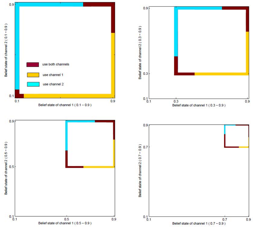
Figure 3 shows the AMPL solution of value function for the following set of parameters: λ0=0.1,λ1=0.9,β=0.9,Rl=2,Rh=3\lambda_{0}=0.1,\lambda_{1}=0.9,\beta=0.9,R_{l}=2,R_{h}=3. The corresponding optimal policy is shown in Figure 4. The structure of the policy in Figure 4 clearly shows the properties we gave in Theorems 1 to 5.
Refer to caption
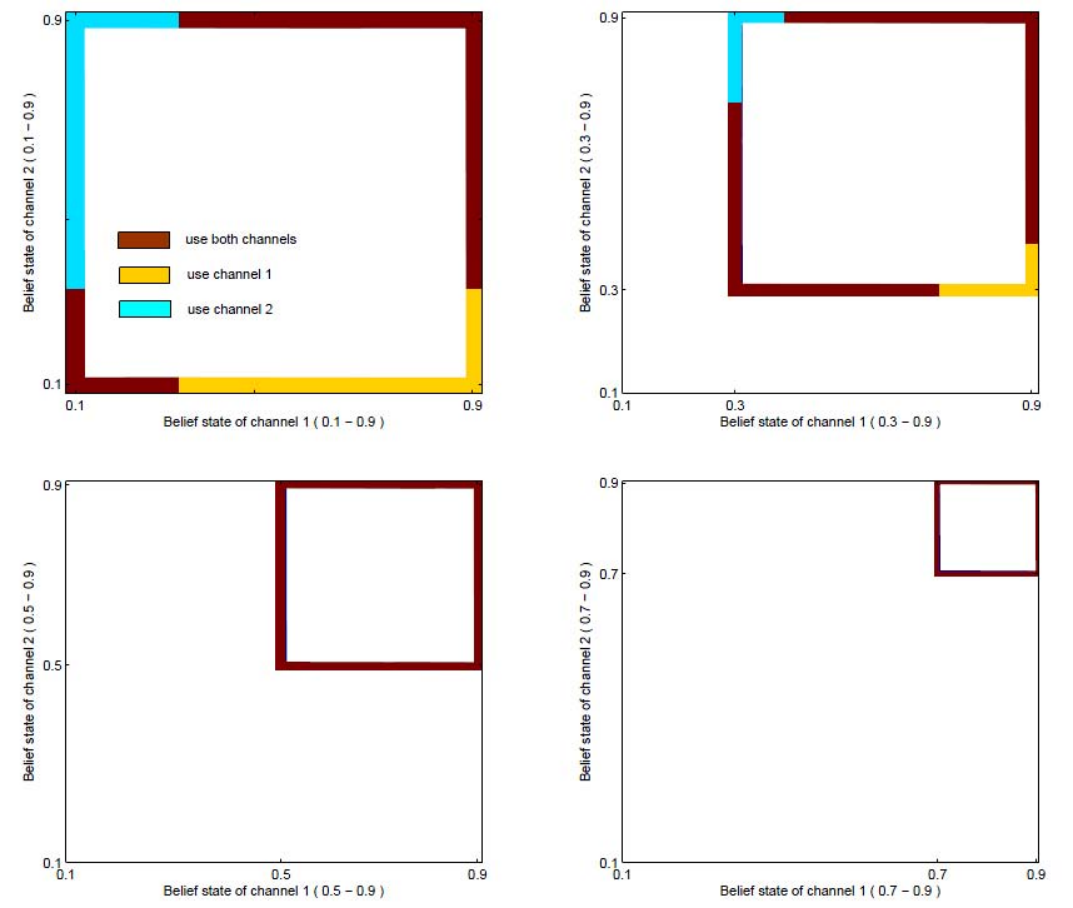
Fig. 5: Optimal policy with increasing λ0\lambda_{0} (Rl=2R_{l}=2, Rh=3R_{h}=3) .

In order to observe the effect of parameters λ0,λ1\lambda_{0},\lambda_{1}, RlR_{l} and RhR_{h} on the structure of optimal policy, we have conducted simulation experiments for varying parameters. First, we increase λ0\lambda_{0} from 0.1 to 0.7, keeping the rest of the parameters the same as in the above experiment. Figure 5 shows the policy structure with different λ0\lambda_{0}. We can observe in Figure 5 that when λ0\lambda_{0} increases from 0.1 to 0.3, the decision region of action BbB_{b} occupies a bigger part of the belief space. Whilst when λ0\lambda_{0} is 0.5 or greater, the whole belief space falls in the decision region of action BbB_{b}, meaning that it is optimal to always use both channels in the set of this experiment when λ0>0.5\lambda_{0}>0.5.

Refer to caption
Fig. 6: Optimal policy with increasing λ0\lambda_{0} (Rl=2,Rh=3.8R_{l}=2,R_{h}=3.8).

Intuitively we believe the optimal policy is closely related to the immediate reward of the three actions. Therefore, in the next experiment, we set RhR_{h} to 3.8 (2=Rl<Rh=3.8<2​Rl2=R_{l}<R_{h}=3.8<2R_{l}) and repeat the above experiment, and the result is shown in Figure 6. Compared to Figure 5, the most obvious difference is that there is no zero-threshold policy structure in Figure 6. This is because when the immediate reward of using one channel is greater (bigger RhR_{h} ), it is more beneficial to use one channel than using both channels.
Refer to caption
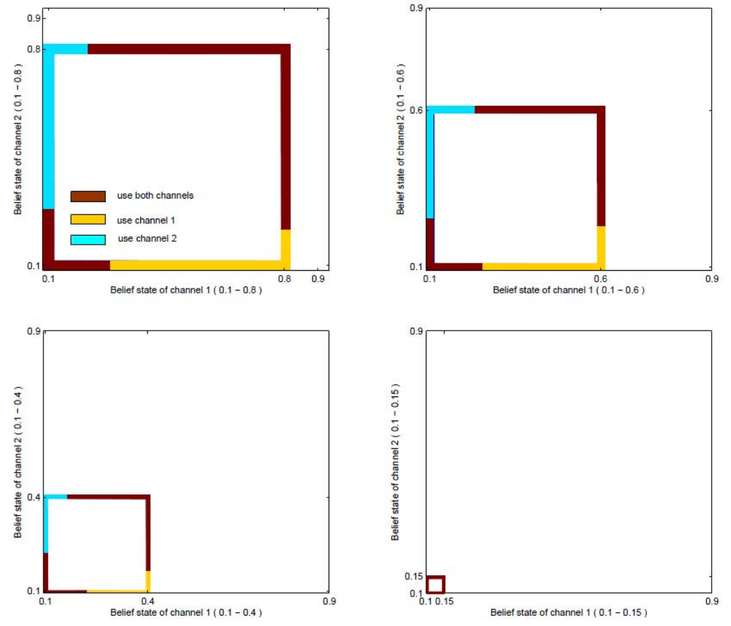
Fig. 7: Optimal policy with decreasing λ1\lambda_{1} (Rl=2,Rh=3.8R_{l}=2,R_{h}=3.8).

Figure 7 shows the structure of optimal policy when λ1\lambda_{1} decreases from 0.9 to 0.15. Other parameters in this experiment are: λ0=0.1,Rl=2,Rh=3,β=0.9\lambda_{0}=0.1,R_{l}=2,R_{h}=3,\beta=0.9. As in Figure 5, both two-threshold and zero threshold policies are observed in this experiment.

Fig. 8: Normalized threshold ρ1\rho_{1} and ρ2\rho_{2} with different β\beta. (λ0=0.1,λ1=0.9\lambda_{0}=0.1,\lambda_{1}=0.9)

From the above observation we understand that the thresholds are sensitive to the value of RlR_{l} and RhR_{h}. Therefore, next we try to observe the relationship between the thresholds and the value of RlR_{l} and RhR_{h}. Figure 8 shows the normalized thresholds ρ1\rho_{1} and ρ2\rho_{2} versus the ratio of RhR_{h} and RlR_{l}, with different discount factor β\beta, when λ0=0.1,λ1=0.9\lambda_{0}=0.1,\lambda_{1}=0.9. ρ1\rho_{1} is normalized as (ρ1−λ0)/(λ1−λ0)(\rho_{1}-\lambda_{0})/(\lambda_{1}-\lambda_{0}), representing the relative length of ΦBbp2=λ0\Phi_{B_{b}}^{p_{2}=\lambda_{0}}. Similarly, the normalized ρ2\rho_{2}, that is, (λ1−ρ2)/(λ1−λ0)(\lambda_{1}-\rho_{2})/(\lambda_{1}-\lambda_{0}), is the relative length of ΦBbp2=λ1\Phi_{B_{b}}^{p_{2}=\lambda_{1}}. It is clear to see that when the normalized threshold ρ1\rho_{1} is 1 (ρ2\rho_{2} is also 1), it corresponds to the zero threshold structure of the optimal policy. From Figure 8 we can also observe that the structure of the optimal policy is affected by the value of the discount factor β\beta.

Fig. 9: Normalized threshold ρ1\rho_{1} and ρ2\rho_{2}. (β=0.8\beta=0.8)

Figure 9 shows the normalized threshold ρ1\rho_{1} and ρ2\rho_{2} with different values of λ0\lambda_{0} and λ1\lambda_{1}. Figure 9 gives us a whole picture of the structure of the optimal policy for different Rh/RlR_{h}/R_{l} and different size of the belief space. We can see that in all experiments with a wide range of parameters, no other policy structure than zero-threshold and two-threshold structure is observed. So we can conclude that with the help of linear-programming simulation, once the five parameters are known (λ0,λ1,Rl,Rh,β\lambda_{0},\lambda_{1},R_{l},R_{h},\beta), the thresholds can be derived based on Figure 9 and the exact optimal policy can be constructed.

V Conclusion

In this paper we have shown the structure of the optimal policy by theoretical analysis and simulation. Knowing that this problem has a 0 or 2 threshold structure reduces the problem of identifying optimal performance to finding the (only up to 2) threshold parameters. In settings where the underlying state transition matrices are unknown, this could be exploited by using a multiarmed bandit (MAB) formulation to find the best possible thresholds (similar to the ideas in the papers [9] and [10]). Also, we would like to investigate the case of non-identical channels, and derive useful results for more than 2 channels, possibly in the form of computing the Whittle index [17], if computing the optimal policy in general turns out to be intractable.

Acknowledgment

This work is done when Junhua Tang is a visiting scholar at USC. The authors would like to thank Yi Gai and Yanting Wu for their helpful discussions. This work is partially supported by Natural Science Foundation of China under grant 61071081 and 60932003. This research was also sponsored in part by the U.S. Army Research Laboratory under the Network Science Collaborative Technology Alliance, Agreement Number W911NF-09-2-0053, and by the Okawa Foundation, under an Award to support research on “Network Protocols that Learn”.

References

  • [1] T. Yoo and A. Goldsmith, “Capacity and power allocation for fading mimo channels with channel estimation error,” IEEE Transactions on Information Theory, vol. 52, pp. 2203–2214, May 2006.
  • [2] W. Yu, W. Rhee, S. Boyd, and J. M. Cioffi, “Iterative water-filling for gaussian vector multiple-access channels,” IEEE Transactions on Information Theory, vol. 50, no. 1, pp. 145–152, 2009.
  • [3] I. Zaidi and V. Krishnamurthy, “Stochastic adaptive multilevel waterfilling in mimo-ofdm wlans,” in 39th Asilomar Conference on Signals, Systems and Computers, 2005.
  • [4] X. Wang, D. Wang, H. Zhuang, and S. D. Morgera, “Energy-efficient resource allocation in wireless sensor networks over fading tdma,” IEEE Journal on Selected Areas in Communications (JSAC), vol. 28, no. 7, pp. 1063–1072, 2010.
  • [5] Y. Gai and B. Krishnamachari, “Online learning algorithms for stochastic water-filling,” in Information Theory and Applications Workshop (ITA 2012), 2012.
  • [6] Q. Zhao, B. Krishnamachari, and K. Liu, “On myopic sensing for multi-channel opportunistic access: Structure, optimality, and performance,” IEEE Transactions on Wireless Communications, vol. 7, no. 12, pp. 5431–5440, 2008.
  • [7] S. H. A. Ahmad, M. Liu, T. Javidi, Q. Zhao, and B. Krishnamachari, “Optimality of myopic sensing in multi-channel opportunistic access,” IEEE Transactions on Information Theory, vol. 55, no. 9, pp. 4040–4050, 2009.
  • [8] A. Laourine and L. Tong, “Betting on gilbert-elliot channels,” IEEE Transactions on Wireless communications, vol. 9, pp. 723–733, February 2010.
  • [9] Y. Wu and B. Krishnamachari, “Online learning to optimize transmission over unknown gilbert-elliot channel,” in WiOpt, 2012.
  • [10] N. Nayyar, Y. Gai, and B. Krishnamachari, “On a restless multi-armed bandit problem with non-identical arms,” in Allerton, 2011.
  • [11] R. D. Smallwood and E. J. Sondik, “The optimal control of partially observable markov processes over a finite horizon,” Operations Research, vol. 21, pp. 1071–1088, September-October 1973.
  • [12] S. M. Ross, Applied Probability Models with Optimization Applications. San Francisco: Holden-Day, 1970.
  • [13] E. J. Sondik, “The optimal control of partially observable markov processes over the infinite horizon: Discounted costs,” Operations Research, vol. 26, pp. 282–304, March/April 1978.
  • [14] D. P. D. Farias and B. V. Roy, “The linear programming approach to approximate dynamic programming,” Operations Research, vol. 51, pp. 850 – 865, November-December 2002.
  • [15] “Neos server for optimization.” http://neos.mcs.anl.gov/neos/.
  • [16] R. Fourer, D. M. Gay, and B. W. Kernighan, AMPL: A Modeling Language for Mathematical Programming. Brooks/Cole Publishing Company, 2002.
  • [17] P. Whittle, “Multiarmed bandits and the gittins index,” Journal of the Royal Statistical Society, vol. 42, no. 2, pp. 143–149, 1980.